Experiments and computations of microfluidic liquid–liquid flow patterns†
Pierre
Desir‡
a,
Tai-Ying
Chen‡
a,
Mauro
Bracconi
 c,
Basudeb
Saha
 b,
Matteo
Maestri
 c and
Dionisios G.
Vlachos
 *ab
*ab
aDepartment of Chemical and Biomolecular Engineering, University of Delaware, 150 Academy Street, Newark, Delaware 19716, USA. E-mail: vlachos@udel.edu
bCatalysis Center for Energy Innovation, 221 Academy Street, Newark, Delaware 19716, USA
cLaboratory of Catalysis and Catalytic Processes, Dipartimento di Energia, Politecnico di Milano, Via La Masa 34, 20156 Milano, Italy
First published on 1st October 2019
Abstract
We study two-phase liquid–liquid flow patterns in a 500 μm capillary microchannel for four biphasic systems: ethyl acetate/water, 2-pentanol/water, methyl isobutyl ketone/water, and heptane/water. Flow visualization experiments using laser induced fluorescence (LIF) reveal a total of 7 different flow patterns for all solvent pairs, namely slug flow, droplet flow, slug-droplet flow, parallel, annular, dispersed, and irregular flow. A map of different flow patterns was built to delineate the origin of their formation. We find conventional dimensionless groups are insufficient to uniquely identify the flow patterns. Computational fluid dynamics (CFD) modeling in OpenFOAM shows agreement with the experimental flow patterns for most of the two-phase flows. Principal component analysis reduces the dimensionality of potential descriptors of flow patterns and, unlike prior work using two dimensionless numbers, determines six important features that describe >95% of the variance of the experimental flow patterns. These include the total flow rate, the flow rate ratio between the two phases, the capillary and Ohnesorge numbers of the aqueous phase, and the Weber number and velocity of the organic phase. We build a decision-tree model to further regress the data and identify the critical features and demonstrate an accuracy in predicting the flow patterns of up to 93%.
Introduction
The advances in microfluidic technology have enabled the effective miniaturization of chemical processes. Continuous flow microreactors with characteristic length scales in the micrometer range (hydraulic diameters <1 mm) possess large surface-to-volume ratios, which result in heat and mass transport rates orders of magnitude greater than bench-scale and conventional reactors. The laminar flow regime and short diffusion time-scale of microreactors allow operation with more precise process windows including heating profiles, residence times, mixing, and reaction times in the order of milliseconds for both single-phase gas and liquid systems.1–3 These characteristics are further enhanced in multiphase microsystems, in particular in liquid–liquid biphasic microreactors, where two immiscible liquids come in contact and generate various two-phase flow patterns by tuning the flow conditions.4–9 The biphasic flow patterns in a microchannel depend on multiple parameters such as the physical properties of the solvents (density, viscosity, and surface tension), the micromixer where the solvent streams intersect, the microchannel wall, diameter, length, and geometry, the flow rate, the fluid velocity, and the fraction of each phase.2,5,8 These flow patterns are usually generated at the inlet of the microchannel using flow focusing geometries and mixing junctions (T-junctions and Y-junctions) as the contacting point of the two liquids.Given the flow rate-range in experimental studies using syringes or reciprocating-piston pumps, the stable flow patterns commonly observed are segmented flow (slug flow and droplet flow) and parallel flow.5 In segmented flow, the two liquids form alternating segments in which the wall-wetting (continuous) phase usually forms a thin film around the non-wetting (dispersed) phase, whereas parallel flow is characterized by the two liquids flowing side by side through the microchannel. The type of flow pattern formed by a solvent pair drives its ultimate application. Slug and droplet flows have extensively been used for synthesis of nanoparticles and for crystallization. In these flow patterns, the dispersed phase is not in contact with the wall and the slug/droplets exhibit strong inner recirculation with no axial dispersion, producing particles with a narrow particle size distribution.2,3,8,10 Segmented flow has also been heavily applied in biology for flow injection analysis, blood analysis, DNA analysis,11 protein isolation, and cell encapsulation.12 Parallel flow has mainly been used in liquid–liquid extraction and characterization of different products, such as metals, metal complexes, ions, and DNA.13–16 Furthermore, slug and droplet flows have been found to be suitable for short contact time liquid–liquid extraction with high extraction efficiencies and millisecond time-span kinetic studies with in situ characterization of the reaction network.4,5,7,17–24 For example, liquid–liquid biphasic microreactors have been applied to the production of 5-hydroxylmethyl furfural (HMF), which is a key platform chemical obtained from the acid-catalyzed dehydration of biomass-derived C6 sugars (glucose and fructose) in water, to prevent the side reactions and increase the HMF yield.
To leverage the advantages of different flow patterns for various applications, predicting the liquid–liquid flow patterns for different solvent pairs is vital. Conventionally, dimensionless analysis is applied, and the dimensionless groups are used to predict the flow patterns for different systems. Darekar et al.25 and Yagodnitsyna et al.26 have investigated various maps of patterns using different dimensionless groups and proposed combinations of them that are suitable for mapping the flow patterns. However, these maps still fail to predict flow patterns at certain operating conditions. Since the conventional method of mapping the flow patterns using dimensionless groups is insufficient to predict flow patterns, CFD is a good alternative for flow pattern predictions providing also insights into the mechanism of their formation.27 Kashid and Agar28 have utilized CFD to investigate the influence of flow rate, channel diameter and Capillary number to the flow regimes and slug size in a liquid–liquid capillary microreactor. On the other hand, Ghaini et al.29 combined experiments and CFD to provide insights into the effects of the contact angle and the interfacial tension on the slug length and the slug formation time using multiple organic solvents. Moreover, Nekouei and Vanapalli30 have investigated the influence of the viscosity ratio and the flow rate ratio between the two solvents on the droplet size using CFD in a microchannel. In this context, CFD simulations can be employed as numerical experiments which can reveal both the resulting flow conditions and the controlling parameters for the pattern generation. However, CFD is computationally intensive. Rapid prediction of the flow patterns corresponding to certain solvents and operating conditions might be achieved by employing machine learning methodology. As a powerful data-driven computational tool, machine learning could also be applied to learn the flow patterns from a dataset and serve as a robust tool for prediction and classification problems. Das and Samanta31 have applied artificial neural networks to predict flow patterns for gas–liquid system with 95% accuracy. Furthermore, Nandagopal and Selvaraju32,33 published several papers on using multiple neural network techniques to predict flow patterns for liquid–liquid systems with an accuracy of ∼95%. Nonetheless, these works mostly focused on utilizing different descriptors, such as superficial velocity and confluence angle, to build a neural network model for only one liquid–liquid system but not for various solvent pairs.
The aim of this paper is to investigate the possibility of using CFD and machine learning techniques to improve the predictive ability of liquid–liquid flow patterns for multiple solvents in capillaries. First, we experimentally study the two phase liquid–liquid flow patterns for four organic solvents with water relevant to HMF extraction,34 ethyl acetate (EtAc), 2-pentanol, MIBK, and heptane. Second, we simulate the various flow patterns using CFD and compare them to our experimental data. Finally, we combine experiments and machine learning techniques to predict the two-phase flow patterns with 93% accuracy. We find that the system is inherently of higher dimensionality of six key descriptors, of which the total flow rate and the capillary number of the aqueous phase are the most important ones.
Methods
Experimental methods
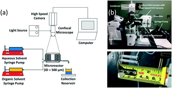
Two syringe pumps (Harvard Apparatus PHD2000 and New Era Pump Systems Inc. NE-300) were used to pump the aqueous and organic solvent feeds into a 500 μm square cross-section T-junction (Valco Instruments) made of polyether ether ketone (PEEK). The details of internal structure of T-junction are provided in the Supplementary material. The feeds intersect in a cross-flow configuration at the T-junction to generate the biphasic flow patterns. The biphasic mixture then enters a capillary microchannel made of perfluoroalkoxy alkane (PFA) tubing (Idex Health) with alternating coiled and straight segments of ID = 500 μm and OD = 1600 μm. Deionized water (Milli-Q) was used as the aqueous solvent. EtAc 99% (Sigma Aldrich), 2-pentanol 99% (Sigma Aldrich), MIBK 99% (Sigma Aldrich), and n-heptane 99% (Sigma Aldrich) were used as the organic solvents. Sodium fluorescein 99% (Sigma Aldrich) and 9,10-diphenylanthracene 99% (Sigma Aldrich) were used as the aqueous fluorescent dye and the organic fluorescent dye, respectively, in order to contrast the two liquid phases during flow visualization.The biphasic flow patterns were characterized using laser induced fluorescence (LIF) of a 250 μM solution of sodium fluorescein in water and a 10 mM of 9,10-diphenylanthracene solution in one of the selected organic solvents, using a high-speed confocal microscope (Highspeed LSM 5 Live Duo) mounted with an inverter. Two laser sources with wavelength of 488 nm and 405 nm were used for the fluorescence excitation of the aqueous and organic solvents, respectively. Images were captured using a Zeiss 1.25× and a 2.5× Plan-Neofluar objective lens at frame rates ranging from 30 to 108.1 fps. Further image analysis and processing of the flow patterns were conducted in ImageJ (Scheme 1).
Computational methods
CFD simulations of two-phase flow are conducted using the single-field incompressible Navier–Stokes equations modeled with the volume-of-fluid (VOF) method.35 The VOF model is a surface-tracking technique using a fixed mesh system to resolve sharp interfaces. A set of single-field equations is employed to describe the fluid dynamics of two-phase flows, which are obtained by means of conditional volume-averaging of the local instantaneous conservation equations of mass and momentum. The location of the interface is obtained from an indicator function (α), which is equal to the volume fraction of a phase in each cell. The solution of the continuity equation eqn (2) for the volume fraction (α) of one of the phases enables to track the evolution of the interphase surface35 | (1) |
 | (2) |
It is worth noticing that the equation is exact because no assumptions are employed in its derivation. The relative velocity is usually modelled as a compressive velocity normal to the interface with a magnitude proportional to the maximum velocity of the field.36 The compressive velocity acts to compensate the numerical diffusion across the interface and is calculated according to eqn (3)
 | (3) |
| ∇(U) = 0 | (4) |
 | (5) |
| Fst = σκ ∇α | (6) |
 | (7) |
A special treatment is required for the cells near the walls where the adhesion force is considered using a fixed contact angle at the liquid/liquid/solid triple point.37 According to the CSF model, the unit normal vector is computed at the walls as a function of the contact angle as in eqn (8)
n = nw![[thin space (1/6-em)]](https://www.rsc.org/images/entities/char_2009.gif) cos cos![[thin space (1/6-em)]](https://www.rsc.org/images/entities/char_2009.gif) θ0 + tw θ0 + tw![[thin space (1/6-em)]](https://www.rsc.org/images/entities/char_2009.gif) sin sin![[thin space (1/6-em)]](https://www.rsc.org/images/entities/char_2009.gif) θ0 θ0 | (8) |
In the VOF method, we solve only the single continuity and momentum equations for the entire domain, an approach known as the “one-fluid” approach.38 Therefore, the variables and material properties are defined as volume-averaged of the two phases in each cell, as shown in eqn (9) and (10)
| ρ = αρ1 + (1 − α)ρ2 | (9) |
| μ = αμ1 + (1 − α)μ2. | (10) |
The governing equations are solved with the finite-volume based, open-source CFD toolbox, OpenFOAM.39 The simulation mesh is established as a 3D T-shape micromixer as shown in Scheme 2, which shares the same geometric parameters and flow conditions with our experimental study. Herein, the channel size is set to 0.5 mm. A total of 1![[thin space (1/6-em)]](https://www.rsc.org/images/entities/char_2009.gif) 856
856![[thin space (1/6-em)]](https://www.rsc.org/images/entities/char_2009.gif) 000 cells within the simulation domain were used, and results regarding flow pattern and slug length are found to be independent of discretization; additional information can be found in the Supplementary material. The dispersed phase, water, flows into the T-mixer from one inlet, while the continuous organic phase, e.g., EtAc, flows into the T-mixer from the other inlet and mixes with the water. The maximum Courant number is set to 0.25 to control the time step without reducing the accuracy and quality of the simulation. Zero gradient for pressure and no-slip boundary condition for velocity are implemented at the wall of the microchannel, and the contact angle is set to be 180°. At the inlet, a zero pressure gradient and constant velocity are used as boundary conditions. At the outlet, the velocity and volume fraction are set to be zero-gradient, and the pressure to be atmospheric.
000 cells within the simulation domain were used, and results regarding flow pattern and slug length are found to be independent of discretization; additional information can be found in the Supplementary material. The dispersed phase, water, flows into the T-mixer from one inlet, while the continuous organic phase, e.g., EtAc, flows into the T-mixer from the other inlet and mixes with the water. The maximum Courant number is set to 0.25 to control the time step without reducing the accuracy and quality of the simulation. Zero gradient for pressure and no-slip boundary condition for velocity are implemented at the wall of the microchannel, and the contact angle is set to be 180°. At the inlet, a zero pressure gradient and constant velocity are used as boundary conditions. At the outlet, the velocity and volume fraction are set to be zero-gradient, and the pressure to be atmospheric.
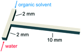 | ||
| Scheme 2 Flow configuration of the organic and aqueous feeds into the T-junction used for both the flow visualization experiments and the CFD simulations. | ||
Results and discussion
Liquid–liquid flow patterns
Fig. 1 shows the two-phase flow patterns observed experimentally among a total of 260 data flow visualization points collected. Overall, 7 different biphasic flow patterns are obtained: slug flow, droplet, slug-droplet, dispersed, parallel, annular, and irregular flow. The flow patterns were visualized in both coiled and straight segments of the microchannel and there were no observable effects of centrifugal forces arising from the channel curvature on the flow patterns. The organic solvent is the continuous phase in most flow patterns (slug, droplet, slug-drop, parallel, annular, and irregular flows) as it wets the hydrophobic microchannel wall while the aqueous solvent (red phase in Fig. 1) is the dispersed phase. However, in the case of the dispersed flow, water is the continuous phase into which the organic solvent is dispersed.40 The slug and droplet flow regimes are marked by elongated slugs and droplets of uniform and constant size and shape. When the length of the dispersed phase segments is longer than the inner diameter, we define the flow pattern as slug flow; when it is equal or shorter than the inner diameter, as droplet flow. The slug-drop and dispersed flows consist of alternating slugs and droplets with non-uniform size. The parallel flow is characterized by a layer of water flowing next to a layer of organic solvent whereas in the annular flow regime, the aqueous layer flows in between two parallel layers of organic solvent. In the irregular flow regime, the dispersed aqueous phase flows as varying deformed slugs and droplets in the organic solvent.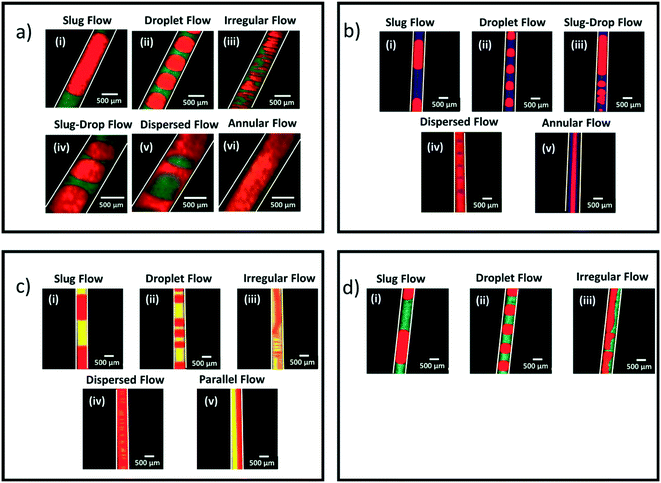 | ||
| Fig. 1 LIF images of the experimental biphasic flow patterns observed for EtAc (green) (a), 2-pentanol (blue) (b), MIBK (yellow) (c), and heptane (cyan) (d). In all the images, water is shown as the red phase. Conditions: Total volumetric flow rate from 0.1 to 10 mL min−1, org/aq (v/v) from 0.25 to 4. The detailed conditions are indicated in Fig. 2. | ||
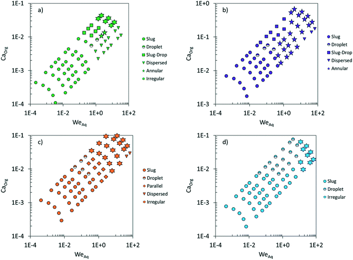
Fig. 2 maps the flow conditions that generate the biphasic flow patterns. Interestingly, for the same total volumetric flow rate and org/aq (v/v) ratio, different organic solvents generate different flow patterns. At low flow rates (<1 mL min−1), the slug flow is the prevalent for all solvent pairs. At high flow rates (>1 mL min−1), the irregular flow is more frequently observed with EtAc and MIBK, the annular flow is dominant with 2-pentanol, and the droplet flow is preferred with heptane. Moreover, parallel flow is only observed when MIBK is used as an organic solvent. Furthermore, the dispersed flow regime is usually encountered at high flow rates and low org/aq (v/v) ratios where the inertial forces in the aqueous phase overcome the surfaces forces in the organic phase, resulting in the aqueous solvent wetting the hydrophobic wall.40
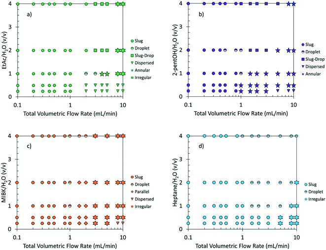 | ||
| Fig. 2 Maps of flow patterns vs. the org/aq (v/v) ratio and the total volumetric flow rate using various organic solvents: EtAc (a), 2-pentanol (b), MIBK (c), heptane (d). | ||
CFD modeling of flow patterns
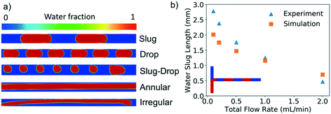
We adopt the same configuration employed in the experimental study (Scheme 2) to assess the capabilities of CFD in predicting the flow patterns. By alternating the flow rate and flow rate ratio between organic and aqueous phase, we analyzed the experimental behavior via numerical simulations. The properties of the solvents employed in CFD are reported in Table 1. Our results revealed the prediction of five different flow patterns, namely slug, droplet, slug-drop, annular, and irregular, as shown in Fig. 3a. The flow patterns are generally in agreement with experimental results under the same conditions for all the solvents considered. At low flow rates, the interfacial tension forces dominate, enabling the sharp formation of slugs at the T-junction section.41,42 We quantitatively assessed the model predictions for this flow pattern by comparing the slug length at different flow rates at unitary flow rate ratio. The slug length in the simulations is evaluated by drawing the isocontour at 0.5 of volume fraction (aqueous phase) to isolate the slug, and then, the actual length is measured using Paraview. Fig. 3b shows that the experimental and numerical results are in good agreement with relative deviations at most of 25%. The slug length decreases as the flow rate increases due to the gradual reduction of the relative importance of the surface tension which turns to be less effective in building long slugs as the inertial and viscous contributions become more relevant.As the flow rate increases, the viscous force increases and starts playing a vital role in the pattern formation. At this condition, the interfacial tension force is not sufficient for breakup, and shear-off takes place after some distance from the T-junction to form a droplet41,42 as shown in Fig. 3a. When the flow rate is high and the inertial force is large enough, the breakup no longer happens and annular flow forms,2 which is accurately predicted by the numerical simulation, as well as the slug-droplet flow regime is observed, which appears only at a high organic-to-aqueous flow rate ratio, as shown in Fig. 3a. In this case, the organic flow rate is sufficiently large giving rise to segments of different size because the slugs are no longer stable. At the very high flow rate, rather irregular flow appears, as shown in Fig. 3a.
Comparison between the numerical simulations and the experimental data reveals an accuracy of 68% of the CFD in predicting the correct pattern. Fig. 4 shows a confusion matrix for each of the solvent. Each element of the confusion matrix represents the fraction of experimental flow patterns (x-axis labels) predicted by CFD (y-axis labels). Diagonal (off diagonal) elements represent correct (incorrect) predictions. For example, the 1st row/3rd column element 0.19 in Fig. 4a means that 19% of the slug flows (1st row) seen experimentally are predicted to be annular by CFD (3rd column). Most of the wrong predictions are related to the dispersed flow which is never forecasted by the simulations. The remaining errors are related to the misprediction of the slug flow at both low flow rate ratio (0.25) and low total flow rate. The prediction errors are related to distinct reasons in the two cases stemming from the limitations of the current model.
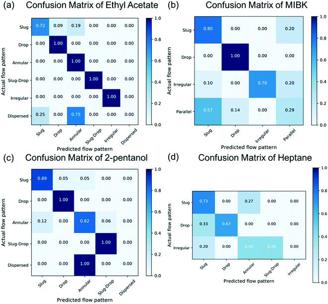 | ||
| Fig. 4 Confusion matrix showing the accuracy of CFD in predicting the flow patterns in the microchannel for EtAc (a), MIBK (b), 2-pentanol (c), and heptane (d). | ||
The dispersed flow is experimentally observed at low flow rate ratios and high total flow rate. In the experiment, it has been noticed that the water is actually wetting the hydrophobic wall due to the large flow rate compared to the organic phase (low flow rate ratio). In this scenario, the continuous and dispersed phase are reversed with respect to the other experiments because of the particular operating conditions, even if the channel walls are hydrophobic. This finally results in a boundary condition mismatch between simulations and experiments. Indeed, the simulation setup imposes a hydrophobic wall due to the nature of the material used in the experiments, using a fixed and pre-defined contact angle whose value is constant in time according to the current surface tension model, i.e., the wettability of the wall does not change during a simulation. This boundary keeps the organic phase touching the wall and avoids the water becoming the continuous phase, thereby preventing the proper prediction of this flow pattern from the simulation. To confirm this hypothesis, we carried out a dedicated simulation using a hydrophilic wall. In doing this, we observed the formation of the dispersed flow as expected from the experiments. CFD simulations are able to reproduce the flow pattern even for this condition. However, they could not be used as a predictive tool since they require knowledge on which phase wets the wall.
The misprediction of the slug flow is confined in the region of low flow rate ratio and low total flow rate. In these cases, the annular flow is predicted from the simulation. These conditions are dominated and governed by the surface tension force since the low fluid velocity keeps the contribution of the viscous and inertial force low. The misprediction could be attributed to an under-prediction of the surface tension force between the two phases. As a result, annular flow is obtained since the surface tension is not sufficient for breaking up the water phase. This indicates that an improvement of the current surface tension model might to be needed to precisely predict these specific flow patterns.
In summary, CFD simulation is a good tool to provide useful information in designing the actual microreactor and understanding the mechanism for flow pattern generation.30,45,46 It is widely used for Taylor flow regime,27,30,45–48 but exposes some limitations in predicting the conditions of different flow patterns observed in experiments. Moreover, CFD simulations are computationally expensive preventing fast screening of different conditions. It takes around 12 to 20 hours computing time using 36 CPUs (Intel E5-2695V4) on a high-performance computing cluster to obtain one flow pattern. Thus, it is important to develop an alternative tool to accurately and quickly predict flow patterns for different conditions and water/organic solvent pairs.
Map of flow patterns
The micro-flow system is mainly influenced by surface forces, viscous forces, and inertial forces. To better understand the dynamics of the forces, four key dimensionless groups are introduced, namely the Reynolds number (Re), the Capillary number (Ca), the Weber number (We), and the Ohnesorge number (Oh). The solvent properties in Table 1 are used in the following equations (their physical interpretation is also shown) to estimate their values: | (11) |
 | (12) |
 | (13) |
 | (14) |
Flow maps, plotting the various patterns vs. one or two dimensionless numbers for both the continuous and dispersed phase, are typically employed for understanding the dynamics of the surface, viscous, and inertial forces and predicting flow patterns. Fig. 5 shows the experimentally observed flow patterns for the various biphasic systems under similar flow conditions vs. the Capillary number of the organic phase (the continuous phase for most of the flow patterns), CaOrg, and the Weber number of the aqueous phase (the dispersed phase in most cases), WeAq. For all organic solvents used, slug flow is obtained at CaOrg < 0.01 and WeAq < 1. These data underscore the fact that slug flow is characterized by strong surface forces. Nonetheless, the maximum Ca number below which slug flow occurs depends on the organic solvent: slug flow is obtained up to CaOrg ∼ 0.1 for 2-pentanol and WeAq ∼ 2 for heptane, reflective of relatively stronger viscous forces in the 2-pentanol/water system and stronger inertial forces in the heptane/water system. Furthermore, at the same values of CaOrg and WeAq, different organic solvents generate different flow patterns. For example, in Fig. 3, at WeAq = 1 and CaOrg = 0.02, EtAc produces droplet flow, 2-pentanol generates slug flow, MIBK forms parallel flow, and heptane forms droplet flow. These observations suggest that the common dimensionless numbers are inadequate to encompass the force dynamics in both solvents of a biphasic system. Flow maps, like Fig. 5, are limited in accurately predicting the flow patterns since CaOrg does not account for the contribution of the inertial forces in the organic phase and WeAq does not consider the relative strength of the viscous forces in the aqueous phase.
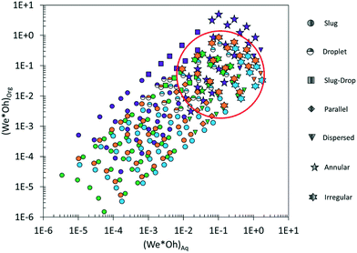
The above observations clearly show that biphasic flow patterns are multi-dimensional systems that depend on the physical properties of the solvents, the flow rate, the flow rate ratio, the common dimensionless numbers, the microchannel diameter, the channel wall, and the contacting geometry. To mitigate the limitations in predicting biphasic flow patterns in microchannels, a universal map of patterns vs. the WeOh product of each phase was developed by Yagodnitsyna and coworkers.26Fig. 6 shows the flow map of experimental patterns for the four biphasic systems used in this study. Slug flow is well described for all organic solvents for (WeOh)Org < 0.003 for the organic phase and (WeOh)Aq < 0.01 for the aqueous phase, which is in the range of WeOh values reported by Yagodnitsyna et al.26 However, this universal map fails at accurately predicting the flow patterns observed at higher WeOh values, as shown in Fig. 6. The red circle highlights the considerable overlap of different flow patterns at similar WeOh values. This again indicates the need for an alternative tool to accurately and quickly predict flow patterns at different conditions and water/organic solvent pairs.
Principal component analysis (PCA)
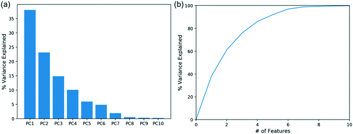
PCA is a useful statistical tool for dimensionality reduction and analysis.49 It can identify the dimensionality of the problem and show potential correlations, and is fairly simple to use. Considering material properties and dimensionless groups of both aqueous and organic phases, there are 19 features in total, shown in Table 2, selected for our analysis. The explained variance of each principal component is shown in Fig. 7a, and the cumulative explained variance in Fig. 7b. The top 2 principal components only explain 38% and 23% of the variance, respectively, and the variance explained by the top 6 principal components is significantly higher than the remaining. Hence, at least 6 features are needed to describe >95% of the variance of the data. Unlike prior work using two dimensionless groups to describe flow patterns, it is clear that PCA suggests that the problem is of higher dimensionality. Since principal components are linear combinations of the original features, it is hard to directly identify the key descriptors and characterize the flow pattern. Another method is therefore needed to efficiently predict the patterns as well as to identify the relevant descriptors.| Features | |
|---|---|
| Aqueous phase (Aq) | Kinematic viscosity (nu), density (rho), velocity (V), Capillary number (Ca), Reynolds number (Re), Weber number (We), Ohnesorge number (Oh) and We × Oh |
| Organic phase (Org) | Kinematic viscosity, density, velocity, Capillary number, Reynolds number, Weber number, Ohnesorge number and We × Oh |
| System-wide | Interfacial tension (sigma), total flow rate (Q), flow rate ratio (Org/Aq) |
Decision tree model
Decision tree learning is a tree-based predictive modeling for regression and classification that provides interpretive predictions.50–52 As a commonly used supervised machine learning method in data mining, decision tree could assist in predicting either the value (regression) or the class (classification) of target variable(s) from input observations.53 Since our variables are discrete, we employ classification trees. To construct a decision tree, the dataset is split into different subsets by choosing certain variables that could best split the set of observations at each node of the tree. The building process of a simple decision tree is illustrated in the ESI.†The Gini impurity is employed to each candidate subset to evaluate the quality of the split and decide the variable for splitting data. The Gini impurity is the measure that a randomly chosen data point would be incorrectly classified by randomly using one of the distributions of classes in the subset.51–53 Here k represents the number of classes and pi represents the fraction of elements that are classified as class i. The split that minimizes the Gini impurity for a system is chosen to divide the dataset and construct the tree. This process is repeated on each subset recursively to build a decision tree until reaching stopping criteria, i.e., every subset contains only one unique class. Then, the averaged Gini impurity decreases for each variable in a node over the entire tree and can be used to estimate the variable importance.51 The decision tree algorithm is carried out using scikit-learn, which is a well-known open-source machine learning package in Python.54
The response space in our problem contains different flow patterns, and the predictors are features selected from Table 2. There is a total of 260 data points collected, and the data is randomly split into a training set and a testing set; 80% of data is used for training and the remaining 20% is kept for testing. A 3-fold cross validation is applied during model training to avoid overfitting. The testing data is used to evaluate the performance of the model. The decision tree model is built using the same features, listed in Table 2. Fig. 8a shows the confusion matrix of the flow pattern predictions and Fig. 8b shows the feature importance. Fig. 8a shows the decision tree model reaches 87% overall accuracy among all flow patterns. The model correctly predicts the slug-drop flow, dispersed flow, and parallel flow. On the other hand, the drop flow is the most wrongly predicted. This may be attributed to the very narrow operating condition window of the drop flow. This pattern has been observed in a very limited number of operating conditions, which in some cases overlaps with the other flow regimes. The machine learning algorithm thereby predicts the drop flow as the common slug or the slug-drop flow in some cases. Besides, the top 6 important features are identified from the feature importance using the decision tree model. These include the total flow rate, the Capillary number of aqueous phase, the Weber number of the organic phase, the flow rate ratio, the velocity of the organic phase, and the Ohnesorge dimensionless group of the aqueous phase. The total flow rate and flow rate ratio are identified as the most important factors that influence patterns, consistent with these being the key variables we tune to obtain different flow patterns. Moreover, the Capillary number of the aqueous phase and the Weber number of the organic phase are identified as vital factors as well, indicating that whether the system is dominated by surface tension force is important for dictating the flow patterns. Using the top 6 important features to build the decision tree model again, the confusion matrix of new model (Fig. 9a) and the evaluation metrics are shown in Fig. 9b, where the F1 score is the harmonic average of precision and recall. The precision is the number of true positives divided by the true positives plus false positives.55 The recall is the correct identifications of the class over the total population of the class.55 The new decision tree model reaches 93% accuracy and correctly predicts slug flow, annular flow, slug-droplet flow, dispersed flow, and parallel flow. The accuracy and F1 score are improved due to reduced overfitting. This indicates that these are the key features of controlling flow patterns. The decision tree model reaches much higher accuracy (>90%) by identifying the key features for this classification problem.
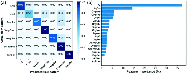 | ||
| Fig. 8 Confusion matrix of decision tree model (a) and feature importance (b). Symbols are defined in Table 2. | ||
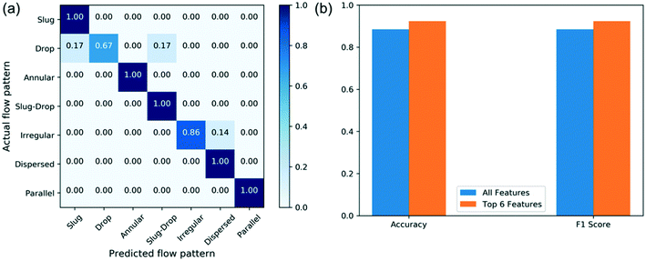 | ||
| Fig. 9 Confusion matrix of the decision tree model (a) and performance of the decision tree model (b). | ||
The methodology of using a decision tree to predict flow pattern could also be extended to liquid–liquid microchannels with hydrophilic walls and gas–liquid systems. When the channel wall is changed from hydrophobic to hydrophilic, the organic phase will become the dispersed phase and the aqueous phase will then be the continuous phase, and different flow patterns might be generated under the same flow conditions. On the other hand, for gas–liquid systems, there would be significant density and surface tension differences, leading to the greater range of dimensionless numbers. In general, the key features identified in this study would also be important in these systems, since these same parameters are tuned by varying operating conditions and determine when the surface tension force dominates. However, the relative importance of key features may differ because of the much different range of dimensionless numbers and operating conditions.
Conclusions
Two-phase flow patterns were studied in a microchannel for systems of relevance to the reactive extraction of HMF, using 4 different organic/aqueous biphasic systems, with water as the aqueous phase and organic solvents including EtAc, 2-pentanol, MIBK, and heptane. The various biphasic flow regimes were generated using a T-junction and were studied experimentally using LIF flow visualization. In total, 7 different two-phase flow patterns were observed: slug flow, droplet flow, slug-drop flow, parallel flow, annular flow, dispersed flow, and irregular flow. Maps for the different flow patterns were created for different flow conditions and all solvent pairs. Interestingly, different flow patterns were observed for different organic solvents under similar flow conditions. Nonetheless, the slug flow regime was found to be common to all solvent pairs at low flow rates <1 mL min−1. The flow patterns were, then, modeled using CFD simulations with fairly good agreement with the experimental results for most of the flow patterns. However, dispersed flow and slug flow at low flow rate ratio are usually wrongly predicted by numerical simulations. In the former, the specific operating conditions, i.e. large amount of water, determines that water is in contact with the wall, an aspect not captured by simulations where as wall is assumed to be hydrophobic. In the latter, the flow is governed by the surface tension due to the very small capillary number. In this case, the closure model for the surface tension plays a vital role for the accurate description of patterns. The model employed in this work is found to under-predict the surface tension resulting in misprediction of this flow pattern.Finally, the flow patterns were analyzed using various descriptors to delineate the physics of flow pattern formation. Using the two common dimensionless groups of Weber number and Ohnesorge number results fails in uniquely identifying the patterns. Principal component analysis determines the most important features and shows that at least 6 features are necessary to explain >95% of the variance of the experimental data. A decision-tree model was then built to further analyze the data and provide insights into the most important features. The model improved the accuracy in predicting flow patterns up to 93% and exposed six critical features that include the total flow rate, the flow rate ratio between the two phases, the Capillary and Ohnesorge numbers of the aqueous phase, and the Weber number and velocity of the organic phase. This work introduces machine learning in accurately describing complex flow patterns to increase the ability to predict liquid–liquid flow patterns and reduce the computational cost compared to using CFD simulations. Moreover, this work underscores that these systems are inherently of higher dimensionality than thought before.
Conflicts of interest
There are no conflicts to declare.Acknowledgements
Funding from the RAPID manufacturing institute, supported by the Department of Energy (DOE) Advanced Manufacturing Office (AMO), award number DE-EE0007888-7.6, is gratefully acknowledged. RAPID projects at the University of Delaware are also made possible in part by funding provided by the State of Delaware. The Delaware Energy Institute gratefully acknowledges the support and partnership of the State of Delaware in furthering the essential scientific research being conducted through the RAPID projects.References
- M. Hoffmann, M. Schluter and N. Rabiger, Chem. Eng. Sci., 2006, 61, 2968–2976 CrossRef CAS.
- C. X. Zhao and A. P. J. Middelberg, Chem. Eng. Sci., 2011, 66, 1394–1411 CrossRef CAS.
- Y. C. Zhao, G. W. Chen and Q. Yuan, AIChE J., 2006, 52, 4052–4060 CrossRef CAS.
- S. L. Anna, N. Bontoux and H. A. Stone, Appl. Phys. Lett., 2003, 82, 364–366 CrossRef CAS.
- N. Assmann, A. Ladosz and P. R. von Rohr, Chem. Eng. Technol., 2013, 36, 921–936 CrossRef CAS.
- G. F. Christopher and S. L. Anna, J. Phys. D: Appl. Phys., 2007, 40, R319–R336 CrossRef CAS.
- A. L. Dessimoz, L. Cavin, A. Renken and L. Kiwi-Minsker, Chem. Eng. Sci., 2008, 63, 4035–4044 CrossRef CAS.
- A. Gunther and K. F. Jensen, Lab Chip, 2007, 7, 399–399 RSC.
- K. Wang, L. Li, P. Xie and G. Luo, React. Chem. Eng., 2017, 2, 611–627 RSC.
- B. K. H. Yen, N. E. Stott, K. F. Jensen and M. G. Bawendi, Adv. Mater., 2003, 15, 1858–1862 CrossRef CAS.
- M. A. Burns, B. N. Johnson, S. N. Brahmasandra, K. Handique, J. R. Webster, M. Krishnan, T. S. Sammarco, P. M. Man, D. Jones, D. Heldsinger, C. H. Mastrangelo and D. T. Burke, Science, 1998, 282, 484–487 CrossRef CAS PubMed.
- S. Sugiura, T. Oda, Y. Izumida, Y. Aoyagi, M. Satake, A. Ochiai, N. Ohkohchi and M. Nakajima, Biomaterials, 2005, 26, 3327–3331 CrossRef CAS PubMed.
- M. Surmeian, A. Hibara, M. Slyadnev, K. Uchiyama, H. Hisamoto and T. Kitamori, Anal. Lett., 2001, 34, 1421–1429 CrossRef CAS.
- H. Hisamoto, T. Horiuchi, M. Tokeshi, A. Hibara and T. Kitamori, Anal. Chem., 2001, 73, 1382–1386 CrossRef CAS.
- Y. Kikutani, H. Hisamoto, M. Tokeshi and T. Kitamori, Lab Chip, 2004, 4, 328–332 RSC.
- V. Reddy and J. D. Zahn, J. Colloid Interface Sci., 2005, 286, 158–165 CrossRef CAS.
- A. Adamo, P. L. Heider, N. Weeranoppanant and K. F. Jensen, Ind. Eng. Chem. Res., 2013, 52, 10802–10808 CrossRef CAS.
- A. Ghaini, M. N. Kashid and D. W. Agar, Chem. Eng. Process., 2010, 49, 358–366 CrossRef CAS.
- J. Jovanovic, E. V. Rebrov, T. A. Nijhuis, M. T. Kreutzer, V. Hessel and J. C. Schouten, Ind. Eng. Chem. Res., 2012, 51, 1015–1026 CrossRef.
- M. N. Kashid, Y. M. Harshe and D. W. Agar, Ind. Eng. Chem. Res., 2007, 46, 8420–8430 CrossRef CAS.
- P. Mary, V. Studer and P. Tabeling, Anal. Chem., 2008, 80, 2680–2687 CrossRef CAS PubMed.
- D. Tsaoulidis and P. Angeli, Chem. Eng. J., 2015, 262, 785–793 CrossRef CAS.
- A. Woitalka, S. Kuhn and K. F. Jensen, Chem. Eng. Sci., 2014, 116, 1–8 CrossRef CAS.
- M. Shang, T. Noël, Y. Su and V. Hessel, AIChE J., 2017, 63, 689–697 CrossRef CAS.
- M. Darekar, K. K. Singh, S. Mukhopadhyay and K. T. Shenoy, Ind. Eng. Chem. Res., 2017, 56, 12215–12226 CrossRef CAS.
- A. A. Yagodnitsyna, A. V. Kovalev and A. V. Bilsky, Chem. Eng. J., 2016, 303, 547–554 CrossRef CAS.
- D. A. Hoang, V. van Steijn, L. M. Portela, M. T. Kreutzer and C. R. Kleijn, Comput. Fluids, 2013, 86, 28–36 CrossRef.
- M. N. Kashid and D. W. Agar, Chem. Eng. J., 2007, 131, 1–13 CrossRef CAS.
- A. Ghaini, A. Mescher and D. W. Agar, Chem. Eng. Sci., 2011, 66, 1168–1178 CrossRef CAS.
- M. Nekouei and S. A. Vanapalli, Phys. Fluids, 2017, 29, 032007 CrossRef.
- H. Sharma, G. Das and A. N. Samanta, AIChE J., 2006, 52, 3018–3028 CrossRef CAS.
- M. S. Giri Nandagopal and N. Selvaraju, Ind. Eng. Chem. Res., 2016, 55, 11346–11362 CrossRef CAS.
- M. S. G. Nandagopal, E. Abraham and N. Selvaraju, Chem. Eng. J., 2017, 309, 850–865 CrossRef CAS.
- Y. Muranaka, H. Nakagawa, R. Masaki, T. Maki and K. Mae, Ind. Eng. Chem. Res., 2017, 56, 10998–11005 CrossRef CAS.
- C. W. Hirt and B. D. Nichols, J. Comput. Phys., 1981, 39, 201–225 CrossRef.
- E. Berberovic, N. P. van Hinsberg, S. Jakirlic, I. V. Roisman and C. Tropea, Phys. Rev. E: Stat., Nonlinear, Soft Matter Phys., 2009, 79, 036306 CrossRef.
- J. U. Brackbill, D. B. Kothe and C. Zemach, J. Comput. Phys., 1992, 100, 335–354 CrossRef CAS.
- D. Gueyffier, J. Li, A. Nadim, R. Scardovelli and S. Zaleski, J. Comput. Phys., 1999, 152, 423–456 CrossRef CAS.
- H. G. Weller, G. Tabor, H. Jasak and C. Fureby, Comput. Phys., 1998, 12, 620–631 CrossRef.
- D. Tsaoulidis, V. Dore, P. Angeli, N. V. Plechkova and K. R. Seddon, Int. J. Multiphase Flow, 2013, 54, 1–10 CrossRef CAS.
- M. De Menech, P. Garstecki, F. Jousse and H. A. Stone, J. Fluid Mech., 2008, 595, 141–161 CrossRef.
- P. Garstecki, M. J. Fuerstman, H. A. Stone and G. M. Whitesides, Lab Chip, 2006, 6, 437–446 RSC.
- M. Z. Shahid, M. R. Usman, M. S. Akram, S. Y. Khawaja and W. Afzal, J. Chem. Eng. Data, 2017, 62, 1198–1203 CrossRef CAS.
- S. Zeppieri, J. Rodríguez and A. L. López de Ramos, J. Chem. Eng. Data, 2001, 46, 1086–1088 CrossRef CAS.
- L. Dai, W. F. Cai and F. Xin, Chem. Eng. Technol., 2009, 32, 1984–1991 CrossRef CAS.
- D. Y. Qian and A. Lawal, Chem. Eng. Sci., 2006, 61, 7609–7625 CrossRef CAS.
- M. J. Nieves-Remacha, L. Yang and K. F. Jensen, Ind. Eng. Chem. Res., 2015, 54, 6649–6659 CrossRef CAS.
- L. Yang, M. J. Nieves-Remacha and K. F. Jensen, Chem. Eng. Sci., 2017, 169, 106–116 CrossRef CAS.
- E. Lopez-Guajardo, E. Ortiz-Nadal, A. Montesinos-Castellanos and K. D. P. Nigam, Chem. Eng. Commun., 2017, 204, 467–475 CrossRef CAS.
- D. A. C. Beck, J. M. Carothers, V. R. Subramanian and J. Pfaendtner, AIChE J., 2016, 62, 1402–1416 CrossRef CAS.
- T. Hastie, R. Tibshirani and J. H. Friedman, The elements of statistical learning: data mining, inference, and prediction, 2009 Search PubMed.
- G. James, D. Witten, T. Hastie and R. Tibshirani, An introduction to statistical learning: with applications in R, 2013 Search PubMed.
- B. Partopour, R. C. Paffenroth and A. G. Dixon, Comput. Chem. Eng., 2018, 115, 286–294 CrossRef CAS.
- F. Pedregosa, G. Varoquaux, A. Gramfort, V. Michel, B. Thirion, O. Grisel, M. Blondel, P. Prettenhofer, R. Weiss, V. Dubourg, J. Vanderplas, A. Passos, D. Cournapeau, M. Brucher, M. Perrot and É. Duchesnay, J. Mach. Learn. Res., 2011, 12, 2825–2830 Search PubMed.
- M. Sokolova and G. Lapalme, Inf. Process. Manage., 2009, 45, 427–437 CrossRef.
Footnotes |
| † Electronic supplementary information (ESI) available. See DOI: 10.1039/c9re00332k |
| ‡ These authors contributed equally. |
| This journal is © The Royal Society of Chemistry 2020 |

