
 Open Access Article
 This Open Access Article is licensed under a Creative Commons Attribution-Non Commercial 3.0 Unported Licence
Kinetic and spectroscopic responses of pH-sensitive nanoparticles: influence of the silica matrix†
Anne Clasena,
Sarah Wenderothb,
Isabella Tavernarob,
Jana Fleddermannb,
Annette Kraegelohb and
Gregor Jung *a
*a
aBiophysical Chemistry, Saarland University, Campus B2 2, 66123 Saarbrücken, Germany. E-mail: g.jung@mx.uni-saarland.de
bINM – Leibniz-Institute for New Materials, Campus D2 2, 66123 Saarbrücken, Germany
First published on 4th November 2019
Abstract
Intracellular pH sensing with fluorescent nanoparticles is an emerging topic as pH plays several roles in physiology and pathologic processes. Here, nanoparticle-sized pH sensors (diameter far below 50 nm) for fluorescence imaging have been described. Consequently, a fluorescent derivative of pH-sensitive hydroxypyrene with pKa = 6.1 was synthesized and subsequently embedded in core and core–shell silica nanoparticles via a modified Stöber process. The detailed fluorescence spectroscopic characterization of the produced nanoparticles was carried out for retrieving information about the environment within the nanoparticle core. Several steady-state and time-resolved fluorescence spectroscopic methods hint to the screening of the probe molecule from the solvent, but it sustained interactions with hydrogen bonds similar to that of water. The incorporation of the indicator dye in the water-rich silica matrix neither changes the acidity constant nor dramatically slows down the protonation kinetics. However, cladding by another SiO2 shell leads to the partial substitution of water and decelerating the response of the probe molecule toward pH. The sensor is capable of monitoring pH changes in a physiological range by using ratiometric fluorescence excitation with λex = 405 nm and λex = 488 nm, as confirmed by the confocal fluorescence imaging of intracellular nanoparticle uptake.
1. Introduction
Apart from their application in catalysis,1–4 nanoparticles have also been used for drug delivery,5–11 infection treatment,12,13 and cancer therapy or diagnosis.14–17 Their use as a biosensor is exemplified in nanoscopic pH probes,18–24 which allows for retrieving relevant health information. The rapid growth of cancer cells in tumors leads to more acidic conditions within the malignant tissue,25,26 but traditional analytical methods, such as proton permeable microelectrodes, fail to determine the intracellular concentration of H+ because of the complex environment therein and the small sample volume.25 In combination with fluorescence techniques, the use of nanoparticles for analyzing the pH value both in vivo and in vitro may overcome these limitations, making them useful for cancer screening. A large number of pH-negative/positive indicators are available, where fluorescence is either quenched or enhanced upon acidification.27,28 In the present work, the focus is on the use of silica particles as a nanomaterial. For the potential use in vivo, silica nanoparticles possess the beneficial property of slow degradation both in aqueous solutions and in blood plasma with disappearing toxicity.29–32 Although labeled silica nanoparticles with self-calibrating pH detection exist, preferential ratiometric detection is established by a mixture of two or more different fluorophores.22,23,30,31,33–38 In this work, two-channel readout is achieved by a single probe molecule, which provides two reversibly interconverting detection signals. The use of a single probe molecule offers the advantage in which the pH measurement is independent of parameters such as local and irreproducible probe composition or preferential photobleaching of one dye.39Silica nanoparticles can be prepared by various methods such as milling,40,41 aerosol process,42,43 microemulsion processing,44 or sol–gel process.45–48 The sol–gel process became the method of choice because of its mild synthesis conditions, simple control over particle size, and monodispersity. Here, the most convenient method is the Stöber process, which involves the ammonia-catalyzed hydrolysis of tetraethyl orthosilicate (TEOS) as the starting material and the use of a water–ethanol solution as the solvent.46 However, only nanoparticles with sizes larger than 50 nm can be prepared without loss of their monodispersity, whereas smaller particles show large size variations.38 Due to the higher dye load, larger nanoparticles are beneficial for imaging and therapy,11,23 but smaller nanoparticle sizes are preferable for other in vivo applications, e.g., for longer blood circulation half-life and ability to penetrate into and permeate through tissues.37,49 Furthermore, smaller particles facilitate analysis by molecular spectroscopy such as fluorescence correlation spectroscopy (FCS) or absorption spectroscopy. Hence, Hartlen et al. modified the Stöber process: they introduced L-arginine instead of ammonia as the catalysts and biphasic system, comprising cyclohexane and water, to prepare monodisperse silica spheres (diameter as low as 15 nm).47,48 These small monodisperse silica particles were used to examine the influence of the external environment, i.e., the silica matrix, with respect to their use as pH sensors. Suitable pH probes are the derivatives of the hydroxypyrene photoacid. In this work, therefore, an immobilizable derivative of hydroxypyrene was synthesized according to a previously described routine to generate asymmetric hydroxypyrene derivatives50 and subsequently covalently embedded in silica nanoparticles.45 We prepared core nanoparticles (C-NP) and core–shell nanoparticles (CS-NP), where the labeled core was clad by another SiO2 shell; then, we compared the spectroscopic behavior of the probe molecule therein. Due to its very clear solvatochromic behavior and proton sensitivity,51 we selected this dye as the probe for the interaction inside the particle and with the outer medium. In addition, when the hydroxypyrene derivative is in the excited state, a proton can be transferred to a suitable acceptor due to the high photoacidity—the so-called excited-state proton transfer (ESPT)—from which information about the hydrogen-bonding networks in the near surrounding can be obtained.52 As pH-sensitive and reasonably photostable dyes, sulfonated hydroxypyrene derivatives are ideally suited to study the mobility of protons within the nanoparticle core, which is critical for the readout performance as pH probes. Altogether, silanized hydroxypyrene derivatives are ideally appropriate for characterizing the silica matrix. Finally, the application of the formed nanoparticles as pH probes in cell cultures is finally exemplified. The spectroscopic data in the experimental part, obtained by time-resolved and steady-state fluorescence spectroscopies, is elaborated in the discussion section, where the various aspects of pH sensing by encapsulated dyes are examined.
2. Experimental
The synthesis of immobilizable photoacid 5a is shown in Scheme 1. For further details on the synthesis of 5a, see the ESI (Chapter 2 and Fig. S6†). Both unlabeled and labeled C-NP were synthesized according to an earlier work.45 A growth step led to CS-NP,45 where the cladding consisted of an unlabeled silica layer. Only for the cellular experiments (ESI, Chapter 16†), an unstained core was covered with a labeled shell. The preparation and characterization of C-NP and CS-NP (TEM, DLS, and ζ-potential value) are shown in the ESI† (Chapter 3–5†). | ||
| Scheme 1 Syntheses of photoacid 5a and its soluble counterpart 5b for comparison. | ||
2.1 Nanoparticle preparation (see ESI, Chapter 2†)
The nanoparticles were concentrated by centrifugation (Spin-X UF concentrators; MWCO: 10 kDa; corning) prior to performing the spectroscopic experiments. The particles were subsequently diluted in the respective solvents. Centrifugation was necessary as a further purification step and will be explained in more detail in the discussion section.2.2 Steady-state fluorescence spectroscopy (ESI, Chapter 8 and 13†)
The emission and excitation spectra of both nanoparticle fractions were recorded in solvents with varying hydrogen-bonding capabilities (Kamlet–Taft parameter α) to determine the strength and influence of hydrogen bonding in comparison to the known solvatochromic behavior.52 For pKa determination, the excitation spectra of C-NP and CS-NP were measured in different buffer solutions (20 mM HPCE buffer, sodium citrate, and sodium phosphate; Fluka/Honeywell) at various pH values. The fluorescence intensity at the λmax value of the photoacid (ROH) and its conjugate base (anionic, deprotonated form; RO−) were determined at each pH from the raw spectra to separately calculate the molar fraction for each species, as well as the intensity ratio.38,53 Furthermore, the emission spectra of C-NP and CS-NP were measured after the addition of hydrochloric acid. A similar measurement was performed with the particles synthesized and purified in deuterium oxide instead of water. In this case, deuterium chloride was added for acidification.The fluorescence emission and excitation spectra of C-NP and CS-NP were recorded using a JASCO spectrofluorometer FP-6500 (JASCO) in a 1.4 mL quartz cuvette.
2.3 Steady-state fluorescence anisotropy
The loss of fluorescence anisotropy, r, when the transition moments of absorption and emission are roughly parallelly oriented, results from the local mobility of the fluorophore and therefore allows for the verification of the rigid incorporation into a matrix.54–56 In our case of moderate labeling, fluorescence anisotropy should only depend on the self-rotation of the spherical nanoparticle and can be slowed down by increasing the particle size or viscosity of the solvent (Perrin equation [eqn (1)]).54,57
 | (1) |
In this expression, r0 denotes the intrinsic anisotropy of the immobile fluorophore; τfl, the fluorescence lifetime; θ, the rotational correlation time; and Drot, the coefficient of rotational diffusion. Drot corresponds to a rate constant and is related to the Boltzmann constant kB, temperature T, viscosity η, and the value of its hydrodynamic radius, rH, via the Stokes–Einstein–Debye equation [eqn (2)].58
 | (2) |
Steady-state anisotropy was determined with the same fluorescence spectrometer as that used in Section 2.2 using vertical polarization for excitation and both vertical and horizontal polarizations for detection. The depicted spectra were corrected for the grating factor G.54
2.4 Time-correlated single-photon counting (TCSPC) and fluorescence quantum yield determination
According to the work of Strickler–Berg, τfl is inversely proportional to the square of the refractive index.59 Hence, τfl values can be used to retrieve information about the refractive index n0, especially when the fluorescence quantum yield, φfl, is high.60 More precisely, the n0 value of any surrounding can be determined according to eqn (3), where water can be used as the reference medium. Here, nx and τx denote n0 and τfl in another medium, respectively. A calibration fit, where the refractive index ncalculated [determined by using eqn (3)] was compared with the refractive index nmeasured, as directly measured with an Abbe refractometer (Atago, 3T) (ESI, Table S6†); this proved the reliability of this procedure.
 | (3) |
Furthermore, TCSPC with excitation of the acidic form (ROH) can be used to characterize the ESPT from the excited photoacid to the nearby solvent molecules.52 The full photochemical cycle following the photon absorption is known as the Förster cycle and is described in detail for pyranine-derived photoacids elsewhere.50–53,61 ESPT in protic solvents is drastically slowed down when replacing water with methanol.52 Similarly, the ESPT efficiency in deuterium oxide is lower by a factor of 2 to 5 than in that in water due to the kinetic isotope effect.62,63 The kinetics of ESPT, which can also be determined from the steady-state experiments, are a sensitive measurement tool for the maintenance of hydrogen-bonding networks.64
Here, φfl was measured on an absolute PL quantum yield spectrometer (C11347, Hamamatsu) in the scan mode.
2.5 FCS
FCS curves were determined using a custom-built setup (ESI, Chapter 12†). The correlation data were analyzed according to a previously described 2D diffusion model, including one or several dark states [eqn (4)].50,65 Here, g(τ) denotes the obtained correlation function of the fluorescence fluctuations and N denotes the apparent particle number.
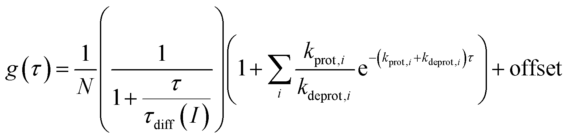 | (4) |
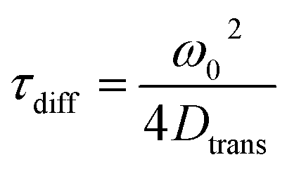
The longest time component of the autocorrelation decay should correspond to the diffusion time, τdiff, of the molecule through the detection volume [eqn (5)].54
 | (5) |
Here, ω0 is the lateral extension of the confocal volume (ω0 = 0.46 μm), which was determined with rhodamine 110 (R110). R110 was selected as the reference because of its superior photostability, its use in single-molecule experiments, and its similar spectroscopic properties to the deprotonated form of compound 5a (see ESI, Fig. S21d†).66,67 Further, Dtrans denotes the coefficient of translational diffusion and is further related to kB, T, η, and rH via the Stokes–Einstein–Debye equation [eqn (6)].58
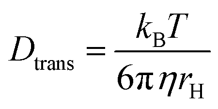 | (6) |
However, τdiff can appear smaller due to any light-driven, irreversible process like photobleaching, which competes with diffusion.65 The occurrence of photobleaching, therefore, is detrimental to any particle size determination by FCS (see ESI, Chapter 12†).
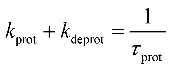
Faster fluorescence fluctuations, described by the second term in eqn (4), arise from the transient dark-state population. As no intensity-dependent dark-state population was noticed, which is in agreement with earlier experiments on this substance class,64,68 the dark-state population exclusively results from the pH-dependent interconversion of the deprotonated dye (RO− form) and protonated dye (ROH form). The parameter kprot in eqn (4) describes the population of the dark-state ROH (protonation) and kdeprot is the depopulation rate constant of the dark state (deprotonation).64,68 However, eqn (4) is valid for molecular species like 5a/b; the preexponential factor kprot/kdeprot is reduced if more than one fluorophore per particle contributes to the fluorescence. It should be noted that smaller particle sizes with lower absolute dye loading are beneficial for this purpose. Under these circumstances, however, the exponential decay constant [eqn (7)] is a more reliable parameter to characterize the protonation kinetics. The time constant of the protonation fluctuations, τprot, then corresponds to the reciprocal of the sum of the rate constants kprot and kdeprot and serves only as a qualitative measure for proton mobility.
 | (7) |
At pH values far above pKa, where protonation can be ignored, eqn (4) is reduced to the first term, i.e., diffusion or photobleaching, respectively.
2.6 Cellular experiments
To determine the internalization of nanoparticles by cells, cellular uptake experiments were carried out using the lung carcinoma cell line A549 (ACC-107). A confocal laser scanning microscope (Zeiss LSM 880, Carl Zeiss, Jena, Germany) equipped with Plan-Apochromat 63×/1.4 oil immersion objective was used to visualize the nanoparticles.3. Results
3.1 Syntheses and characterization of label 5a
The synthesis of 5a, starting from 6-/8-bromopyrenol (1), is shown in Scheme 1.50 The mixture of both regioisomers (1) was transformed into the corresponding sulfonesters. At this stage, the two isomers could be separated by chromatography, and the assignment of the substitution pattern of 2 was evident from the X-ray crystallographic analysis (ESI, Fig. S60 and Table S9†). For further syntheses, compound 2 was solely used. The protection of the phenolic moiety is achieved by an allyl group yielding 3, which is cleaved off during the subsequent palladium-catalyzed debromination to compound 4. Finally, 5a and its soluble derivative 5b were obtained after additional sulfonation by chlorosulfonic acid and the subsequent reaction with (3-aminopropyl)triethoxysilane (APTES) or dimethylamine. Following the same strategy, a compound similar to 5a, where 4 was converted with trimethoxy[3-(methylamino)propyl]silane after treatment with chlorosulfonic acid, has been used for immobilization in single-molecule chemistry.69The fluorescence excitation and emission spectra of 5a were measured at various pH values (ESI, Fig. S6 and Table S3†), from which the pKa value of 6.06 ± 0.11 (ESI, Fig. S8 and S10†) was obtained. The excitation and emission spectra of deprotonated 5a in various solvents (ESI, Fig. S22a and S23a†) showed distinct dependence on α, which is in agreement with previously found solvatochromic behavior of constitutionally similar compounds.51 Deprotonated 5a had τfl value of 5.7 ns in water (φfl = 90%), which is similar to other hydroxypyrene derivatives,64 but this value reduced to 4.7 ns in glycerol (Fig. 3a; ESI, Fig. S15†).
3.2 Physicochemical properties of silica nanoparticles
In this work, we adopted the well-known synthesis of unlabeled and labeled C-NP and CS-NP using L-arginine-catalyzed hydrolysis of TEOS in a biphasic water–cyclohexane system.45 In the case of labeled nanoparticles, 5a was incorporated into the silica particle matrix (Scheme 2).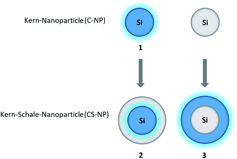 | ||
| Scheme 2 Syntheses of unlabeled and labeled core (C-NP) and core–shell nanoparticles (CS-NP), respectively. | ||
The average particle radius of the obtained unlabeled C-NP was 8.3 ± 0.7 nm (Table 1; ESI, Fig. S1 and Table S2†) and was reproducibly increased by the incorporation of the dye at a radius of about 11.9 ± 1.2 nm. The growth step with an unlabeled shell provides an additional 4–4.5 nm-thick layer in both the cases. Here, the unmarked and modified CS-NP finally have radii of about 12.4 ± 1.2 and 16.3 ± 1.2 nm, respectively. The TEM images reveal that all the synthesized nanoparticles are spherical and fairly monodisperse (dispersity < 10%).
| Unlabeled C-NP | Labeled C-NP | Unlabeled CS-NP | Labeled CS-NP | |
|---|---|---|---|---|
| rTEM [nm] | 8.3 ± 0.7 | 11.9 ± 1.2 | 12.4 ± 1.2 | 16.3 ± 1.2 |
| rDLS [nm] | 9 ± 1 | 17 ± 2 | 15 ± 2 | 23 ± 7 |
| ζ-Potential [mV] | −29.6 ± 3.1 | −43.0 ± 0.5 | −34.4 ± 0.9 | −42.4 ± 0.8 |
DLS revealed that the mean rH value for unlabeled C-NP was 9 ± 1 nm and that for modified particles was 17 ± 2 nm (ESI, Fig. S3†). Unlabeled CS-NP exhibited a mean rH value of 15 ± 2 nm and the dye-embedded CS-NP had a mean rH value of 23 ± 7 nm (Table 1; ESI, Fig. S3 and Table S2†).
Unlabeled C-NP showed a negative ζ-potential value of −29.6 ± 3.1 mV, whereas the modified C-NP exhibited an even more negative ζ-potential value with absolute values of −43.0 ± 0.5 mV (Table 1; ESI, Fig. S5†). The same trend was observed with CS-NP, which became increasingly negative when dye 5a was embedded. Here, the unlabeled CS-NP exhibited a negative ζ-potential value of −34.4 ± 0.9 mV, decreasing to values between −40.3 ± 0.1 mV and −42.4 ± 0.8 mV in nanoparticles containing 5a.
3.3 Steady-state fluorescence spectroscopy
Unlabeled C-NP and CS-NP did not show any fluorescence. For this reason, all the spectroscopic examinations were exclusively conducted with labeled C-NP or CS-NP. Initially, the fluorescence excitation and emission spectra of C-NP and CS-NP at various pH values were used to titrate the dyes within the silica matrix (Fig. 1; ESI, Fig. S8–S13†).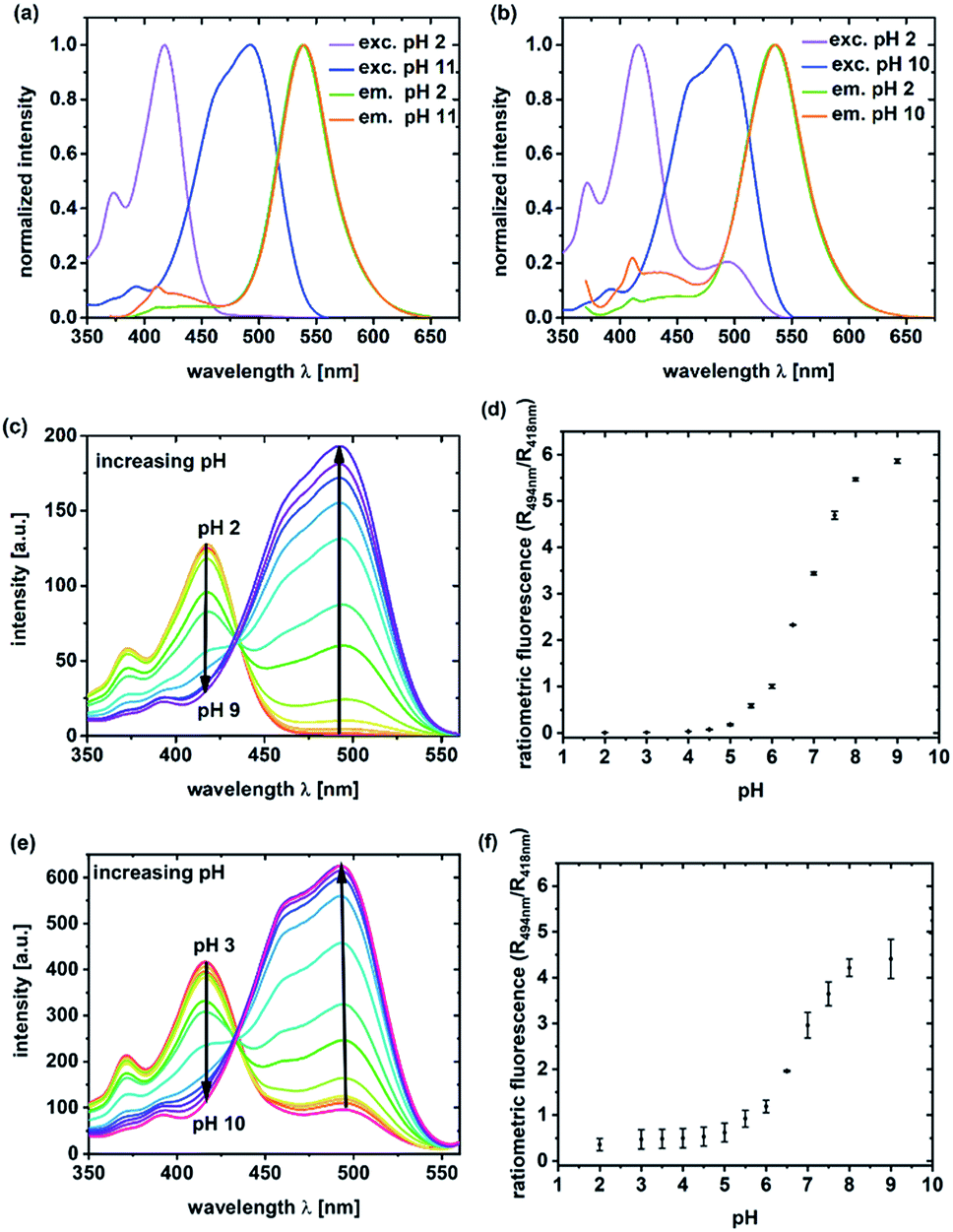 | ||
| Fig. 1 Excitation (exc.) (λem = 570 nm) and emission spectra (em.) (λex = 360 nm) of C-NP (a) and CS-NP (b) at pH 2 (ROH) and 11 or 10, respectively (RO−); excitation titration (λdet = 570 nm) of C-NP (c) and CS-NP (e) at various pH values. The corresponding fluorescence intensity ratios are shown in (d) and (f) and are averaged over three independent measurements. | ||
It turned out that the spectroscopic maxima were hardly affected by the additional silica layer (ESI, Table S3†), and both C-NP and CS-NP showed an isosbestic point in their excitation spectra, too (Fig. 1c and d). The pKa values of 6.08 and 6.15 were obtained for the titratable fractions (ESI, Table S4†), and are close to that of free dye 5a (pKa = 6.06). However, the dye within the CS-NP still showed a basic form at pH < 4, which appears to not be titratable down to pH 2 (Fig. 1e) and remained even after acidification with a strong acid (ESI, Fig. S19b†). Similarly, the dynamic range of the fluorescence intensity ratio is reduced. W (Fig. 1d vs. Fig. 1f). We will provide a tentative explanation for this peculiar behavior below (in Section 4.2) by investigating the similarity to fluorescent proteins.
3.4 Steady-state fluorescence anisotropy measurements
Fluorescence anisotropy experiments were performed to examine the mobility of immobilized 5a. For quantitative analysis, r was calculated at λexcmax (495 nm ± 5 nm). Based on eqn (2) and the rH data from DLS (Table 1), the expected θ value in water was larger for C-NP (4.5 μs) and CS-NP (10 μs) and therefore much longer than the typical θ value of smaller molecules (8–17 ps).70 Although the exact value of θ could not be determined (see ESI, Fig. S17†), it is obvious that θ is much longer than τfl and a high value (r ≫ 0) is expected for tightly bound or embedded dye molecules. In agreement with these considerations, C-NP showed higher anisotropy (rC-NP ≈ 0.22) than unbound dye 5b (r5b ≈ 0) (Fig. 2a; ESI, Fig. S14†), which could be enhanced after another centrifugation step, but then remained constant (rC-NP ≈ 0.30). CS-NP showed comparatively higher anisotropy after the centrifugation step, too (rCS-NP ≈ 0.32). The anisotropy of both the nanoparticle fractions could be increased by adding glycerol (rC-NP ≈ 0.40 and rCS-NP ≈ 0.39) (Fig. 2b). The filtrate after centrifugation, however, showed fluorescence and lower anisotropy, which was comparable to unbound dye 5b.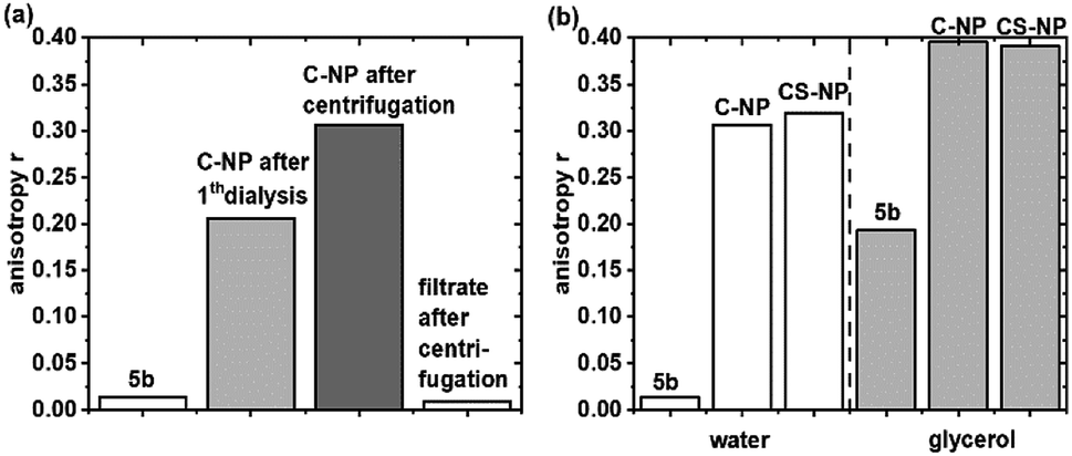 | ||
| Fig. 2 Steady-state fluorescence anisotropy of C-NP in water (a) and 5b and C-NP and CS-NP in water and after the addition of glycerol (b) at λexcmax (495 nm ± 5 nm). | ||
3.5 TCSPC and fluorescence quantum yield
The deprotonated species of the dye in C-NP and CS-NP had τfl values of 5.5 and 5.2 ns, respectively (ESI, Fig. S15†), which is slightly higher than the decay of free dye 5a in water (τfl = 5.7 ns). The fluorescence quantum yield, however, remained constant at a high value (φfl = 89 ± 1%). After immersion into glycerol, the τfl value even further dropped to τfl = 4.7 ns for 5a and τfl = 4.6 ns for both the nanoparticle fractions (ESI, Fig. S15†). Unbound dye 5a showed the clear dependence of τfl on the refractive index (Fig. 3a; ESI, Table S6†). Therefore, τfl, determined by TCSPC, can be used to calculate the refractive index of the environment, where n0 = 1.36 ± 0.02 and n0 = 1.40 ± 0.02 for C-NP and CS-NP, respectively.71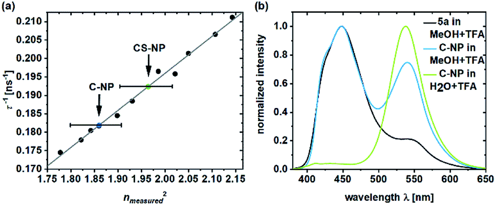 | ||
| Fig. 3 Inverse fluorescence lifetime of 5a in the system with water/glycerol versus the square of the measured refractive index (ESI, Table S6†).71 The refractive indexes of 5a in C-NP (blue dot) and CS-NP (green dot) were determined on the basis of the linear fit (a). Emission spectra of 5a and C-NP after acidification in various solvents (b). Please note that all the τfl values are obtained from the monoexponential fits. | ||
As already shown in Fig. 1, ESPT still occurs in C-NP and CS-NP after acidification (Fig. 3b, green line; ESI, Fig. S19b†). Interestingly, molecular precursor 5a in methanol barely shows ESPT after acidification (Fig. 3b, black line), whereas a significantly higher fluorescence intensity of the deprotonated form (RO−) as a result of ESPT was observed for C-NP in MeOH (Fig. 3b, blue line). The kinetics of ESPT was also investigated by performing time-resolved experiments in both C-NP and CS-NP after the addition of HCl (ESI, Fig. S16a†). The small amplitudes of the rising component, however, indicate that ESPT is mostly faster than the time resolution of our experiments (ESI, Fig. S16 and Table S5†), despite the distinct emission of the neutral form (ROH) at λem = 400–470 nm (Fig. 3b, green line).
3.6 Protonation kinetics
During the determination of pKa and the observation of ESPT by TCSPC in the previous section, we noticed that in some samples, a shift in the fluorescence intensities and spectra in time could be observed. Obviously, the shift in the equilibrium from deprotonated 5a to neutral 5a is retarded in certain samples. To obtain a further insight into the underlying protonation kinetics, we measured the emission spectra of C-NP and CS-NP in water after strong acidification (Fig. 4a). The emission spectra of C-NP indicated—within our time resolution—the immediate shift from the emission of the protonated form (ROH) to the emission of the deprotonated form (RO−) (not shown). In contrast, the emission spectra of CS-NP showed a slow conversion on a time scale of hours from the deprotonated (RO−) to the protonated (ROH) forms (Fig. 4a; ESI, Fig. S18c†). Similar results were obtained with deuteron instead of proton, although the time constants of the biexponential rise slightly differed (ESI, Fig. S18b and d†).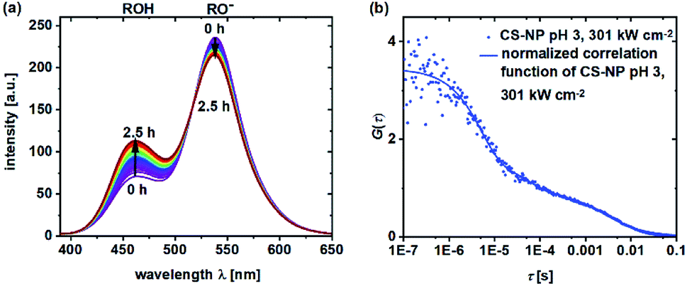 | ||
| Fig. 4 Emission spectra (λex = 360 nm) of CS-NP in H2O after the addition of HCl (t = 2.5 h) (a) and normalized FCS curves of CS-NP at pH 3 and excitation intensity = 301 kW cm−2 (b). | ||
The protonation and deprotonation kinetics were also investigated by FCS, where small dye loading was exploited. FCS experiments were performed at pH ≪ pKa, where distinct fluorescence fluctuations are expected despite an unknown amount of dye molecules per particle. Fluctuations at this pH value reveal a continuous protonation–deprotonation exchange.
Autocorrelation decays, as shown in Fig. 4b, were analyzed according to eqn (4) and (7). At pH 4.5, we obtained τprot = 2.5 ± 0.1 μs for C-NP and τprot = 5.4 ± 0.4 μs for CS-NP; comparatively, τprot = 1.8 ± 0.2 μs for unbound dye 5b, respectively (ESI, Fig. S20b†). FCS measurements of CS-NP, even at pH 3, showed a dark state (Fig. 4b) with τprot (CS-NP) = 3.8 ± 0.2 μs. An additional, reversible process with τprot ∼0.5 ms was detected in these samples, too.
3.7 Solvatochromism
Pyrene derivatives exhibit pronounced solvatochromism, which can be exploited to characterize the surrounding in terms of α.51 As the presence of unreacted, weakly acidic Si–OH in the interior is anticipated, we analyzed the response of deprotonated 5a toward protic solvents. The solvatochromic behaviors of both the nanoparticle types (ESI, Fig. S22 and S23†) were compared to the spectroscopic maxima in solution (Fig. 5).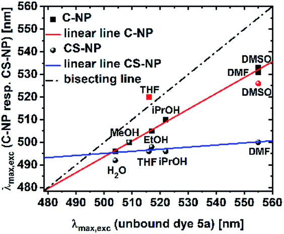 | ||
| Fig. 5 Maxima of the excitation spectra of C-NP and CS-NP vs. unbound dye 5a (red icons were excluded from the linear line). | ||
Modified C-NP still showed dependence on its solvent environment (ESI, Fig. S22b†), but to a lesser extent than that without silica surrounding. No significant, solvent-related changes, with the exception of aprotic DMSO and, less explicitly, DMF, were noticed for CS-NP (ESI, Fig. 22c†). In all these cases, however, the excitation spectra of 5a in the nanoparticles were hypsochromically shifted as compared to those for 5a in a pure solvent (ESI, Fig. S22†).
3.8 Qualitative pH sensing
As a proof of concept, human alveolar epithelial cell line (A549 cells) was used to evaluate the suitability of 5a, embedded in silica NP as a pH sensor for use in live cellular imaging. Confocal microscopy with various excitation lines was performed to qualitatively probe pH (for further details, see ESI, Chapter 16.3†). Depending on the cell compartment, the intracellular pH was 4.5–7.39,72 For these cellular experiments, CS-NP was synthesized with an unlabeled core and labeled shell (Fig. 2 and ESI, Fig. S31 and S32, Table S8†). The used nanoparticles had the same spectroscopic properties and pH response as C-NP shown earlier, but at a larger size (rTEM = 13.7 ± 4.2 nm) and brighter fluorescence. For both the forms of 5a, the neutral state and conjugated base were addressed with λex = 405 nm and λex = 488 nm, respectively. As shown in Fig. 6 and 7, fluorescence emission (λem = 510–550 nm) was observed after incubation with the dye-loaded particles (protonated form = blue; deprotonated form = green). The weak autofluorescence, found in certain cells, did not interfere with the qualitative outcome (ESI,† Fig. S33 and S34†). Outside the cell, both neutral (ROH) and deprotonated (RO−) forms were observed, with higher intensity after RO− excitation (Fig. 6, yellow arrow). When the particles were located in the cells, fluorescence with the excitation of RO− was severely dimmed out and only fluorescence with excitation of ROH was enhanced (Fig. 6, white arrow). Furthermore, the intracellular fluorescence of ROH was co-localized with the red fluorescence from the lysosomes that were stained by LysoTracker™ Red DND-99 (LysoRed; Fig. 7, white arrow).39,73,74 | ||
| Fig. 6 Confocal fluorescence images of A549 cells after 6 h (a) and 24 h (b) of incubation with dye embedded particles (CS-NP) at an applied dose of 100 μg SiO2 per mL. The plasma membrane was stained with tetramethylrhodamine WGA (WGA-TRITC). The images in the first column show the protonated form (ROH, blue) (λex = 405 nm; λem = 510–550 nm) and deprotonated form in the second column (RO−, green) (λex = 488 nm; λem = 510–550 nm). The images in the third column show the staining with WGA-TRITC (red) (λex = 543 nm; λem = 570–650 nm). | ||
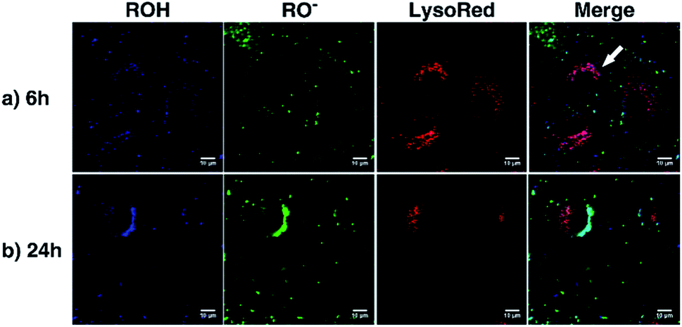 | ||
| Fig. 7 Confocal fluorescence images of A549 cells after 6 h (a) and 24 h (b) of incubation with dye-embedded particles (CS-NP) (applied dose: 100 μg SiO2 per mL). The lysosome was stained with LysoRed. The images in the first column show the protonated form (ROH, blue) (λex = 405 nm; λem = 510–550 nm) and the second column show the deprotonated form (RO−, green) (λex = 488 nm; λem = 510–550 nm). The images in the third column show the staining with LysoRed (red) (λex = 543 nm; λem = 570–650 nm). | ||
4. Discussion
4.1 Particle preparation
In this study, we exploited the beneficial fluorescence properties of pyrene-based photoacids for the development of a pH sensor, while simultaneously characterizing the interior of silica nanoparticles. Moreover, conclusions about nanoparticle preparation could be drawn, too. In general, the incorporation of the dye led to larger particle sizes and hydrodynamic diameters without a significant effect on the spherical particle morphology or dispersity, which is in agreement with the known tendency of labeled nanoparticle precursors to generate larger seeds.75 Then, the subsequent growth step is unaffected by the incorporated dye, which is reflected by an equal increase of 4–4.5 nm in the particle and hydrodynamic sizes. Interestingly, the increase in n0 in CS-NP (from n0(C-NP) = 1.36 ± 0.02 to n0(CS-NP) = 1.40 ± 0.02), as revealed by the τfl measurements (Fig. 3a), provides evidence that SiO2 (n0(fused SiO2) = 1.46 (ref. 76)) not only grows on the outer particle surface but also substitutes H2O within the interior of the nanoparticle during the growth step. A second, reproducible effect of dye incorporation is noticed in the ζ-potential value. The increase in its absolute value through dye embedding was also found for CS-NP and can probably be explained by the additional negative charges of the ionized dye. Furthermore, the higher ζ-potential value indicates higher stability against agglomeration due to electrostatic repulsion.77We determined that earlier purification protocols were insufficient to remove “free” dyes: the measured τdiff value in the range of ∼100 μs indicates the diffusion of unreacted 5a or labeled oligomers (like silsesquioxane).45,78 The removal of “free dye” was accomplished by supplementary purification, by either dialysis for a second time or centrifugation (MW = 10 kDa).
A second, independent proof of incomplete purification was obtained from anisotropy experiments. Similar to τdiff in FCS, the experimentally observed r value was averaged over all the available fluorophores. Here, r ranges from 0.4 for fixed orientation during the fluorescence lifetime [e.g., see the nanoparticles in highly viscous glycerol (Fig. 2b)] to 0 for complete depolarization due to rapid rotation (such as that for 5b). From our experiments, we conclude that anisotropy experiments are superior to FCS measurements in assessing the quality of purification and incorporation, as long as dyes in lower concentrations are embedded within the silica matrix.
4.2 Protonation dynamics
Nanoparticles, loaded with pH-sensitive dyes, were used as pH probes in cells.22–24,38 We, therefore, investigated the pH sensitivity of a hydroxypyrene derivative within the silica matrix.64 The pKa value of 5a (pKa = 6.06 ± 0.11) remained unchanged when incorporated into the silica matrix (pKa = 6.08 ± 0.04) and raised only marginally by an additional cladding layer (pKa = 6.15). However, CS-NP still showed a minor fraction of the basic form even down to pH 2, and FCS measurements at pH 3 revealed protonation–deprotonation equilibrium, evident from the intensity-independent dark state (Fig. 4b). Such a pronounced deviation in the protonation equilibrium from the circumstances in solution, which occurs here at least 3 pH units below the pKa value, has been earlier found in a completely different system of green fluorescent protein (GFP).79 We, therefore, can conclude—on the basis of this similarity—that ∼20% of the dye is stabilized in its basic form by the silica matrix after cladding. This explanation is supported by the ubiquitous hypsochromic shift in the excitation maxima of 5a in all the nanoparticle samples as compared to 5a in the solvents (Fig. 5) and hints to strong hydrogen bonding from Si–OH to RO− in the interior (see below). A direct consequence is a reduction in the dynamic range of the ratiometric output (Fig. 1d and f). It should be noted that our observation also explains the incomplete cancellation of fluorescein fluorescence in pH-sensitive nanoparticles and the variation in the ratiometric signals among different preparations.31,33,34Although a pKa value close to the physiological condition is beneficial for its subsequent use as a biosensor, its quality is crucially affected by the speed upon which the indicator reacts to changes in pH. The addition of HCl or DCl immediately shifts the equilibrium in C-NP, but protons only slowly reach the pH-sensitive moiety of 5a in CS-NP (Fig. 4a; ESI, Fig. S18†). FCS experiments at pH 4.5 (ESI, Fig. S20b†), however, provide the necessary time resolution to follow protonation in C-NP. Again, the shell slowed down the migration of the proton to the fluorescent dye as τprot(C-NP) = 2.5 ± 0.1 μs < τprot(CS-NP) = 5.4 ± 0.4 μs. A comparison with the protonation kinetics of 5a in solution (τprot(5a) = 1.8 ± 0.1 μs) reveals that the protonation kinetics is slightly decelerated even in C-NP, although the equilibrium is not. At this point, it should be emphasized that protonation might be a highly heterogeneous process, at least in CS-NP, as the time constants (5 μs, 0.5 ms, Fig. 4b), as determined by FCS, are far below those determined by cuvette experiments (Fig. 4a).
Data regarding the protonation mechanism can also be obtained from the steady-state fluorescence spectra of acidified nanoparticles. The emission spectra of C-NP and CS-NP predominantly showed the deprotonated form of photoacids in a commercial buffer (ESI, Fig. S13†) as a result of ESPT. Therefore, ESPT was still possible despite the presence of the silica matrix. This finding is noteworthy as methanol effectively suppresses ESPT in solution,52 but not equally strong in the nanoparticles (Fig. 3b). Consequently, we deduce a vastly intact hydrogen-bonding network around incorporated dye 5a, similar to that of the chromophore in wt-GFP.80,81 In summary, the access of protons from the outside to pH-sensitive 5a was possible for both C-NP and CS-NP via a water-like hydrogen-bonding network; in particular, however, the diffusion of protons after the growth step was considerably slowed down and the complete protonation of the chromophore system was no longer possible.
4.3 Accessibility of the chromophore system
The r values of both the nanoparticles (rC-NP ≈ 0.30; rCS-NP ≈ 0.32) as compared to that of unbound dye 5b (r5b ≈ 0) indicates that the photoacid is rigidly incorporated into the silica matrix. Protonation, however, shows that the chromophore in C-NP is accessible for H+ and, to a certain extent, in CS-NP. Therefore, we need to determine the extent to which a firmly embedded indicator is shielded from the exterior. We, therefore, addressed the accessibility of the chromophore system for small-scale interactions other than H+. The influence of molecules with short-range interactions (reff < 1 nm) on both C-NP and CS-NP was studied by solvatochromism and fluorescence quenching via PET by using a small molecule (ESI, Chapter 13 and 14†). The excitation maxima of anionic 5a embedded in the core nanoparticles showed clear dependence on the solvent environment (ESI, Fig. S22b†). Although the trend is qualitatively identical to the observation with the well-studied literature derivatives of hydroxypyrene, with the exception of THF,51 this dependency is only two-third stronger than that of unbound dye 5a (Fig. 5). This finding fits the observation of maintained ESPT, even if protic solvents other than water are used (see preceding section, Fig. 3b).A straightforward explanation for the attenuated dependence on solvent acidity is shielding afforded by the silica matrix. The noticed concomitant blue-shift in the excitation spectra strongly suggests the strong hydrogen-bonding donors. The tendency is even more pronounced in CS-NP where hardly any solvatochromism is found (Fig. 5). Here, the dyes are almost completely shielded from the outer solvent with the exception of dimethyl sulfoxide. This solvent might partially dissolve the nanoparticles.
The impression that a silica environment only provides limited access of the outer environment to the chromophore system is engendered by the lack of fluorescence quenching observed in PET. Obviously, the shell is an efficient barrier for quencher molecules, which contradicts—to some extent—the outcome of the solvatochromism of C-NP. The hydrogen bonding of Si–OH groups to the quencher molecules may explain this discrepancy. To further characterize the sensitivity of the chromophore system to other quenchers with long-range interactions, additional quenching experiments were performed using a FRET quencher with variable action radii rq.38 These experiments revealed that the accessibility of the chromophore system was identical despite cladding by an unstained silica layer (ESI, Fig. S29†). We, therefore, assume the infiltration of the quencher into the nanoparticles. Earlier, the underlying porous structure was already derived from the BET measurements on heavily dried nanoparticles.82–84
4.4 Ratiometric readout
In this work, a two-channel pH probe was prepared with a fast pH response that was comparable to that of an unbound dye in solution. The ratiometric readout was achieved by using a single probe molecule instead of two different chromophore systems as done earlier. The prepared pH sensor, therefore, has an advantage as compared to conventional ratiometric nanoprobes, wherein a heterogeneous and unequal distribution of the indicator cannot be a problem.37 The sensitivity of our probe molecule is also of minor importance as single-molecule detection has been realized earlier.69 Furthermore, the fairly high intensity change upon pH changes simplifies the subsequent analyses and can be, at least partially, traced back to the smaller size as compared to other nanoparticle preparations.31,34–36,85 In addition, the particles consist of hardly toxic components and are smaller than most well-known nanoprobes. Therefore, our particles are ideally suited to track the intracellular pH in living cells as exemplified in live-cellular microscopy. These experiments (Fig. 6 and 7) suggest that CS-NP is sufficiently appropriate for cellular imaging despite its smaller size. Furthermore, the co-localization of LysoRed and the intracellular fluorescence of neutral 5a indicate that the particles were uptaken in acidic compartments such as lysosomes with a pH of 4.5–5 (Fig. 7, white arrow).39,73,745. Conclusions
We synthesized an immobilizable derivative of hydroxypyrene, 5a, which was subsequently used for the preparation of fluorescent silica nanoparticles. The resulting nanoparticles were studied by various fluorescence spectroscopic methods and analyzed with respect to three subjects: preparation, accessibility, and influence of the surrounding on spectroscopic behavior. It was aimed to generate pH-sensitive nanoparticles with pKa values in the physiological range. For C-NP, we found that the silica matrix does not alter the pH sensitivity and only moderately decelerates the protonation kinetics. The insensitivity toward amines, unexpected in the sense that protic solvents can still interact with the chromophore to a certain extent, is beneficial for an application as abundant amines may act as unspecific quenchers in a cellular environment. In contrast, we found out that proton diffusion through an unlabeled, cladding shell (thickness < 10 nm) in CS-NP was considerably retarded. One reason for this is that internal water is partially substituted by SiO2, as indicated by the higher refractive index n0. This is in agreement with the fact that the incorporated photoacid 5a could not be fully protonated despite the low pH values, indicating stabilization of RO− by hydrogen bonding. This weakened susceptibility to external pH entails a reduced dynamic range in the intensity ratio (Fig. 1d vs. 1f). The lack of sensitivity toward the other, directly interacting molecules, therefore, is understandable; consequently, the optical response of CS-NP was largely unaffected by solvents. Interestingly, although the water content of C-NP is presumably reduced to ∼50% in CS-NP, its amount is still sufficient for inducing ESPT within the nanoparticles. In summary, both the silica matrix and unlabeled shell shielded the interior from external influence and provided a beneficial porous structure for the easy access of H+. However, on the basis of our results, only C-NP or CS-NP with labeled shells are suitable for use as ratiometric pH probes with fast pH response due to the almost intact water-like surrounding of 5a.Conflicts of interest
There are no conflicts to declare.Acknowledgements
Financially support by the German Research Foundation (DFG JU650/7-1 and DFG JU650/8-1) is gratefully acknowledged. We also thank Reiner Wintringer (†), Service Center Mass Spectrometry (Saarland University) for recording the mass spectra, Dr Volker Huch (Saarland University) for recording and analysing X-ray crystallographic data, Dr Marcus Koch (INM) for electron microscopy analysis and Dr Emmanuel Teriac (INM) for technical support at confocal fluorescence microscopy. We also thank Nadja Klippel and Guido Kickelbick (Saarland University) for helpful discussion. In addition, we acknowledge support by the German Research Foundation (DFG) and the Saarland University within the funding programme Open Access Publishing.References
- H.-T. Chen, S. Huh, J. W. Wiench, M. Pruski and V. S.-Y. Lin, J. Am. Chem. Soc., 2005, 127, 13305–13311 CrossRef CAS.
- S. Huh, H.-T. Chen, J. W. Wiench, M. Pruski and V. S.-Y. Lin, Angew. Chem., Int. Ed., 2005, 44, 1826–1830 CrossRef CAS.
- C.-Y. Lai, J. Thermodyn. Catal., 2013, 5, e124 Search PubMed.
- Y.-W. Li, L. Dong, C.-X. Huang, Y.-C. Guo, X.-Z. Yang, Y.-J. Xu and H.-S. Qian, RSC Adv., 2016, 54241–54248 RSC.
- I. Slowing, C. Wu, J. Vivero-Escoto and V. Lin, Small, 2009, 1, 57–62 CrossRef.
- I. Slowing, C. Wu, J. Vivero-Escoto and V. Lin, Adv. Drug Delivery, 2008, 60, 1278–1288 CrossRef CAS.
- B. Pelaz, C. Alexiou, R. A. Alvarez-Puebla, F. Alves, A. M. Andrews, S. Ashraf, L. P. Balogh, L. Ballerini, A. Bestetti, C. Brendel, S. Bosi, M. Carril, W. C. W. Chan, C. Chen, X. Chen, X. Chen, Z. Cheng, D. Cui, J. Du, C. Dullin, A. Escudero, N. Feliu, M. Gao, M. George, Y. Gogotsi, A. Grünweller, Z. Gu, N. J. Halas, N. Hampp, R. K. Hartmann, M. C. Hersam, P. Hunziker, J. Jian, X. Jiang, P. Jungebluth, P. Kadhiresan, K. Kataoka, A. Khademhosseini, J. Kopecek, N. A. Kotov, H. F. Krug, D. S. Lee, C.-M. Lehr, K. W. Leong, X.-J. Liang, M. L. Lim, L. M. Liz-Marzán, X. Ma, P. Macchiarini, H. Meng, H. Möhwald, P. Mulvaney, A. E. Nel, S. Nie, P. Nordlander, T. Okano, J. Oliveira, T. H. Park, R. M. Penner, M. Prato, V. Puntes, V. M. Rotello, A. Samarakoon, R. E. Schaak, Y. Shen, S. Sjöqvist, A. G. Skirtach, M. G. Soliman, M. M. Stevens, H.-W. Sung, B. Z. Tang, R. Tietze, B. N. Udugama, J. S. VanEpps, T. Weil, P. S. Weiss, I. Willner, Y. Wu, L. Yang, Z. Yue, Q. Zhang, Q. Zhang, X.-E. Zhang, Y. Zhao, X. Zhou and W. J. Parak, ACS Nano, 2017, 11, 2313–2381 CrossRef CAS.
- Y.-K. Gong and F. M. Winnik, Nanoscale, 2012, 4, 360–368 RSC.
- T. Limnell, H. A. Santos, E. Mäkilä, T. Heikkilä, J. Salonen, D. Y. Murzin, N. Kumar, T. Laaksonen, L. Peltonen and J. Hirvonen, J. Pharm. Sci., 2011, 100, 3294–3306 CrossRef CAS.
- S. Bertoni, Z. Liu, A. Correia, J. P. Martins, A. Rahikkala, F. Fontana, M. Kemell, D. Liu, B. Albertini, N. Passerini, W. Li and H. A. Santos, Adv. Funct. Mater., 2018, 28, 1806175 CrossRef.
- R. Narayan, U. Y. Nayak, A. M. Raichur and S. Garg, Pharmaceutics, 2018, 10, 118 CrossRef CAS.
- B. Gonzáles, M. Colilla, J. Díez, D. Pedraza, M. Guembe, I. Izquierdo-Barba and M. Vallet-Regí, Acta Biomater., 2018, 68, 261–271 CrossRef.
- M. J. Hajipour, K. M. Fromm, A. Akbar Ashkarran, D. Jimenez de Aberasturi, I. Ruiz de Larramendi, T. Rojo, V. Serpooshan, W. J. Parak and M. Mahmoudi, Trends Biotechnol., 2012, 30, 199–511 CrossRef.
- S. Sanchez-Salcedo, M. Vallet-Regí, S. Allaf Shahin, C. A. Glackin and J. I. Zink, Chem. Eng. J., 2018, 340, 114–124 CrossRef CAS.
- H. Mekaru, J. Lu and F. Tamanoi, Adv. Drug Delivery, 2015, 95, 40–49 CrossRef CAS.
- J. Liu, C. Chen, S. Ji, Q. Liu, D. Ding, D. Zhao and B. Liu, Chem. Sci., 2017, 8, 2782–2789 RSC.
- C. Shi, C. Thum, Q. Zhang, W. Tu, B. Pelaz, W. J. Parak, Y. Zhang and M. Schneider, J. Controlled Release, 2016, 237, 50–60 CrossRef CAS.
- A. Sharma, R. Khan, G. Catanante, T. A. Sherazi, S. Bhand, A. Hayat and J. L. Marty, Toxins, 2018, 10, 197 CrossRef.
- R. Gupta and N. K. Chaudhury, Biosens. Bioelectron., 2007, 22, 2387–2399 CrossRef CAS.
- D. Avnir, S. Braun, O. Lev and M. Ottolenghi, Chem. Mater., 1994, 6, 1605–1614 CrossRef CAS.
- X. Le Guével, F. Y. Wang, O. Stranik, R. Nooney, V. Gubala, C. McDonagh and B. D. MacCraith, J. Phys. Chem. C, 2009, 113, 16380–16386 CrossRef.
- X. Wan, D. Wang and S. Liu, Langmuir, 2010, 26, 15574–15579 CrossRef CAS.
- A. Burns, P. Sengupta, T. Zedayko, B. Baird and U. Wiesner, Small, 2006, 6, 723–726 CrossRef.
- D. Wencel, T. Abel and C. McDonagh, Anal. Chem., 2014, 86, 15–29 CrossRef CAS PubMed.
- I. F. Tannock and D. Rotin, Cancer Res., 1989, 49, 4373–4384 CAS.
- L. Feng, Z. Dong, D. Tao, Y. Zhang and Z. Liu, Natl. Sci. Rev., 2018, 5, 269–286 CrossRef CAS.
- R. L. Ragsdale and R. J. Grasso, J. Immunol. Methods, 1989, 123, 259–267 CrossRef CAS.
- J. Thiery, D. Keefe, S. Boulant, E. Boucrot, M. Walch, D. Martinvalet, I. S. Goping, R. C. Bleackley, T. Kirchhausen and J. Lieberman, Nat. Immunol., 2011, 12, 770–777 CrossRef CAS PubMed.
- Y. Zhang, E. M. Stolper and G. J. Wasserburg, Earth Planet. Sci. Lett., 1991, 103, 228–240 CrossRef CAS.
- S.-A. Yang, S. Choi, S. M. Jeon and J. Yu, Sci. Rep., 2018, 8, 185 CrossRef.
- N. D. Mathew, M. D. Mathew and P. P. T. Surawski, Anal. Biochem., 2014, 450, 52–56 CrossRef CAS.
- S. Chandra, G. Beaune, N. Shirahata and F. M. Winnik, J. Mater. Chem. B, 2017, 5, 1363–1370 RSC.
- C.-J. Tsou, C.-H. Hsia, J.-Y. Chu, Y. Hung and Y.-P. Chen, Nanoscale, 2015, 7, 4217–4225 RSC.
- J. Fu, C. Ding, A. Zhu and Y. Tian, Analyst, 2016, 141, 4766–4771 RSC.
- W. Pan, H. Wang, L. Yang, Z. Yu, N. Li and B. Tang, Anal. Chem., 2016, 88, 6743–6748 CrossRef CAS.
- I. Acquah, J. Roh and D. J. Ahn, Macromol. Res., 2017, 25, 950–955 CrossRef CAS.
- X. Huang, J. Song, B. C. Yung, X. Huang, Y. Xiong and X. Chen, Chem. Soc. Rev., 2018, 47, 2873–2920 RSC.
- M. M. Elsutohy, A. Selo, V. M. Chauhan, S. J. B. Tendler and J. W. Aylott, RSC Adv., 2018, 8, 35840–35848 RSC.
- J. Han and K. Burgess, Chem. Rev., 2010, 110, 2709–2728 CrossRef CAS PubMed.
- M. Salavati-Niasari, J. Javidi and M. Dadkah, Comb. Chem. High Throughput Screening, 2013, 16, 458–462 CrossRef CAS.
- N. R. Radhip, N. Pradeeo, M. Abhishek Appaji and S. Varadharajaperumal, Journal of Pure Applied and Industrial Physics, 2015, 5, 165–172 Search PubMed.
- L. Zeng and A. P. Weber, J. Aerosol Sci., 2014, 76, 1–12 CrossRef CAS.
- M. Mezherichera, J. K. Nunes, J. J. Guzowski and H. A. Stone, Chem. Eng. J., 2018, 346, 606–620 CrossRef.
- K. S. Finnie, J. R. Bartlett, C. J. A. Barbé and L. Kong, Langmuir, 2007, 23, 3017–3027 CrossRef CAS.
- S. Schmidt, I. Tavernaro, C. Cavelius, E. Weber, A. Kümper, C. Schmitz, J. Fleddermann and A. Kraegeloh, Nanoscale Res. Lett., 2017, 12, 545 CrossRef.
- W. Stöber, A. Fink and E. Bohn, J. Colloid Interface Sci., 1968, 26, 62–69 CrossRef.
- T. Yokoi, Y. Sakamoto, O. Terasaki, Y. Kubota, T. Okubo and T. Tatsumi, J. Am. Chem. Soc., 2006, 128, 13664–13665 CrossRef CAS.
- K. D. Hartlen, A. P. T. Athanasopoulos and V. Kitaev, Langmuir, 2008, 24, 1714–1720 CrossRef CAS.
- N. Hoshyar, S. Gray, H. Han and G. Bao, Nanomedicine, 2016, 11, 673–692 CrossRef CAS.
- B. Finkler, I. Riemann, M. Vester, A. Grüter, F. Stracke and G. Jung, Photochem. Photobiol. Sci., 2016, 15, 1544–1557 RSC.
- C. Spies, B. Finkler, N. Acar and G. Jung, Phys. Chem. Chem. Phys., 2013, 15, 19893–19905 RSC.
- C. Spies, S. Shomer, B. Finkler, D. Pines, E. Pines, G. Jung and D. Huppert, Phys. Chem. Chem. Phys., 2014, 16, 9104–9114 RSC.
- D. Maus, A. Grandjean and G. Jung, J. Phys. Chem. A, 2018, 122, 9025–9030 CrossRef CAS.
- J. R. Lakowicz, Principles of Fluorescence Spectroscopy, Springer, New York, USA, 4th edn, 2010 Search PubMed.
- B. G. Hosu and C. H. Berg, Biophys. J., 2018, 114, 641–649 CrossRef CAS.
- N. G. James and D. M. Jameson, Methods Mol. Biol., 2014, 1076, 29–42 CrossRef CAS.
- D. M. Jameson and J. C. Croney, Comb. Chem. High Throughput Screen., 2003, 6, 167–176 CrossRef CAS.
- A. Loman, I. Gregor, C. Stutz, M. Mund and J. Enderlein, Photochem. Photobiol. Sci., 2010, 9, 627–636 RSC.
- S. J. Strickler and A. Berg, J. Chem. Phys., 1962, 37, 814–822 CrossRef CAS.
- K. Suhling, P. French and D. Phillips, Photochem. Photobiol. Sci., 2005, 4, 13–22 RSC.
- G. Jung, S. Gerharz and A. Schmitt, Phys. Chem. Chem. Phys., 2009, 11, 1416–1426 RSC.
- E. Pines, Isotope Effects in Chemistry and Biology, Taylor and Francis, Boca Raton, USA 2006, pp. 451–464 Search PubMed.
- O. Gajst, R. Simkovitch and D. Huppert, J. Phys. Chem. A, 2017, 121, 6917–6924 CrossRef CAS.
- B. Finkler, C. Spies, M. Vester, F. Walte, K. Omlor, I. Riemann, M. l Zimmer, F. Stracke, M. Gerhards and G. Jung, Photochem. Photobiol. Sci., 2014, 13, 548 RSC.
- B. Hinkeldey, A. Schmitt and G. Jung, ChemPhysChem, 2008, 9, 2019–2027 CrossRef CAS.
- J. B. Grimm, B. P. English, J. Chen, J. P. Slaughter, Z. Zhang, A. Revyakin, R. Patel, J. Mackling, D. Normanno, R. H. Singer, T. Lionnet and L. D. Lavis, Nat. Methods, 2015, 12, 244–250 CrossRef CAS.
- M. Beija, C. A. M. Alfonso and J. M. G. Martinho, Chem. Soc. Rev., 2009, 38, 2410–2433 RSC.
- M. Vester, A. Grueter, B. Finkler, R. Becker and G. Jung, Phys. Chem. Chem. Phys., 2016, 18, 10281–10288 RSC.
- J. A. Menges, A. Clasen, M. Jourdain, J. Beckmann, C. Hoffmann, J. König and G. Jung, Langmuir, 2019, 35, 2506–2516 CrossRef CAS.
- B. Sinha, D. Bhattacharya, D. K. Sinha, S. Talwar, S. Maharana, S. Gupta, and G. V. Shivashankar, Methods in Cell Biology – Nuclear Mechanics & Genome Regulation, Academic Press, Elsevier, Singapore, 1st edn, 2010, vol. 98, pp. 57–78 Search PubMed.
- K. Suhling, J. Siegel, D. Phillips, P. M. W. French, S. Lévêque-Fort, S. E. D. Webb and D. M. Davis, Biophys. J., 2002, 83, 3589–3595 CrossRef CAS.
- L. He, Y. Li, C.-P. Tan, R.-R. Ye, M.-H. Chen, J.-J. Cao, L.-N. Ji and Z.-W. Mao, Chem. Sci., 2015, 6, 5409–5418 RSC.
- J. A. Mindell, Annu. Rev. Physiol., 2012, 74, 69–86 CrossRef CAS.
- C. Schumann, S. Schübbe, C. Cavelius and A. Kraegeloh, J. Biophotonics, 2012, 5, 117–127 CrossRef.
- A. Imhof, M. Megens, J. H. Engelberts, D. T. N. de Lang, R. Sprik and W. L. Vos, J. Phys. Chem. B, 1999, 103, 1408–1415 CrossRef CAS.
- J. H. Wray and J. T. Neu, J. Opt. Soc. Am., 1969, 59, 774–776 CrossRef CAS.
- K. Pate, and P. Safier, Advances in Chemical Mechanical Planarization (CMP), Woodhead Publishing, Hillsboro, USA 2016, vol. 12, pp. 299–325 Search PubMed.
- N. Hurkes, C. Bruhn, F. Belaj and R. Pietschnig, Organometallics, 2014, 33, 7299–7306 CrossRef CAS.
- L. M. . Oltrogge, Q. Wang and S. G. Boxer, Biochemistry, 2014, 53, 5947–5957 CrossRef CAS.
- M. Chattoray, B. A. King, G. U. Bublitz and S. G. Boxer, Proc. Natl. Acad. Sci. U. S. A., 1996, 93, 8362–8367 CrossRef.
- A. A. Voityuk, M.-E. Michel-Beyerle and N. Rösch, Chem. Phys. Lett., 1997, 272, 162–167 CrossRef CAS.
- D. A. Keane, J. P. Hanrahan, M. P. Copley, J. D. Holmes and M. A. Morris, J. Porous Mater., 2010, 17, 145–152 CrossRef CAS.
- X. G. Qiao, P.-Y. Dugas, L. Veyre and E. Bourgeat-Lami, Langmuir, 2018, 34, 6784–6796 CrossRef CAS.
- H. Peuschel, T. Ruckelshausen, C. Cavelius and A. Kraegeloh, BioMed Res. Int., 2015, 2015, 1–16 CrossRef.
- F. Bruni, J. Pedrini, C. Bossio, B. Santiago-Gonzalez, F. Meinardi, W. K. Bae, V. I. Klimov, G. Lanzani and S. Brovelli, Adv. Funct. Mater., 2017, 27, 1605533 CrossRef.
Footnote |
| † Electronic supplementary information (ESI) available. CCDC 1904703 and 1904704. For ESI and crystallographic data in CIF or other electronic format see DOI: 10.1039/c9ra06047b |
| This journal is © The Royal Society of Chemistry 2019 |