 Open Access Article
Application of ANN modeling techniques in the prediction of the diameter of PCL/gelatin nanofibers in environmental and medical studies
Saba Kalantarya,
Ali Jahani *b,
Reza Pourbabakia and
Zahra Beigzadehc
aDepartment of Occupational Health Engineering, School of Public Health, Tehran University of Medical Sciences, Tehran 1416753955, Iran
bDepartment of Natural Environment and Biodiversity, Faculty of Environment, College of Environment, Karaj 31746118, Iran. E-mail: ajahani@alumni.ut.ac.ir
cEnvironmental Health Engineering Research Center, Kerman University of Medical Sciences, Kerman 7616913555, Iran
First published on 12th August 2019
Abstract
Prediction of the diameter of a nanofiber is very difficult, owing to complexity of the interactions of the parameters which have an impact on the diameter and the fact that there is no comprehensive method to predict the diameter of a nanofiber. Therefore, the aim of this study was to compare the multi-layer perceptron (MLP), radial basis function (RBF), and support vector machine (SVM) models to develop mathematical models for the diameter prediction of poly(ε-caprolactone) (PCL)/gelatin (Gt) nanofibers. Four parameters, namely, the weight ratio, applied voltage, injection rate, and distance, were considered as input data. Then, a prediction of the diameter for the nanofiber model (PDNFM) was developed using data mining techniques such as MLP, RBFNN, and SVM. The PDNFMMLP is introduced as the most accurate model to predict the diameter of PCL/Gt nanofibers on the basis of costs and time-saving. According to the results of the sensitivity analysis, the value of the PCL/Gt weight ratio is the most significant input which influences PDNFMMLP in PCL/Gt electrospinning. Therefore, the PDNFM model, using a decision support system (DSS) tool can easily predict the diameter of PCL/Gt nanofibers prior to electrospinning.
1 Introduction
In recent decades, nanofibers have been proposed as excellent candidates in many areas owing to their unique properties such as their micro or nanoscale structure, high porosity, large surface area to volume ratio, and their substantial mechanical flexibility and strength in the medical and engineering industries, including drug delivery, filtration, tissue engineering, protective clothing, nanoelectronics, nanobiosensors, nanocatalysis, and so forth.1,2 Electrospinning is an easy, versatility, and inexpensive method to prepare polymeric ultrafine fibers under the action of a high electrostatic field from a wide variety of polymers.3,4 Gelatin (Gt) is one of the most common biopolymers, and has been widely explored owing to its biodegradability, biocompatibility, immunogenicity profiles, hydrophilic nature, and commercial availability at a low cost.5 Poly(ε-caprolactone) (PCL) is a semi-crystalline linear hydrophobic polymer which is most commonly used for medical and environmental applications, owing to its biocompatibility and slow biodegradability.6,7 Polymer blending is one of the most effective techniques for providing new or desirable properties such as blending synthetic and natural polymers. Therefore, gelatin can be blended with PCL to improve the biomechanical, degradation, and cell adhesion properties.6Although a wide variety of complicated electrospinning techniques such as coaxial,8 modified coaxial,9 tri-axial,10 side-by-side11 and other complicated techniques12 have been successively reported, only a few limited publications have reported manipulation of the quality of the nanofibers, which is often evaluated by their diameter. Fiber size distribution and morphology play a significant role in the porosity, the surface to volume ratio, functionality, and performance.13 The shape, diameter of the electrospun nanofibers, and spatial distribution have a close relationship with their functional performance and can be divided into four categories: polymer properties (molecular weight and solubility), properties of the working fluids (the concentration, solution viscosity, dielectric properties, surface tension, and conductivity), the operational conditions (applied voltage, the fluid flow rate, nozzle–collector distance, and nozzle diameter of the spinneret), and manipulation of the environmental conditions (temperature, atmospheric pressure, relative humidity, the possible vacuum and even hot air blowing). These parameters have a positive impact on downsizing of the nanofibers.14–18 Despite important experimental investigations to determine fiber diameter, using scanning electron microscopy, transmission electron microscopy, and atomic force microscopy for example, it is still time-consuming and expensive.18,19 Furthermore, complexities in the electrospinning method and many factors simultaneously affecting the preparation techniques cause the findings from statistical tools, such as response surface methodology and regression analysis, to be very noisy.16,20 Regression analysis is one of the traditional techniques that has been used for model generation but the accuracy decreases when the independent parameters increase. In complex phenomena modeling, methods such as an artificial neural network (ANN) are employed.21 An ANN is an attractive and flexible choice for solving linear and nonlinear multivariate regression and different problems because it is based on the natural neural network of the brain.21–23 An ANN consists of interconnected processing elements, such as an input layer, various hidden layers and an output layer which is capable of learning from samples, using transfer functions between neurons and a specific learning algorithm in the structure of a program without being affected by data noise.24–26 Nowadays, different models and learning algorithms can be applied to modeling and controlling the electrospinning processes.27,28 In this paper, we have compared the multi-layer perceptron (MLP), radial basis function (RBF), and support vector machine (SVM) models for predicting the diameter of PCL/gelatin nanofibers. The main objectives were to: (i) analyze the effects of weight ratios, applied voltage, injection rate, nozzle–collector distance, and their individual and interactive effects on the diameter of PCL/gelatin nanofibers; (ii) compare different data mining models to identify the most accurate model; (iii) detect the most significant factors affecting the diameter of PCL/gelatin nanofibers using sensitivity analysis; and (iv) design a decision support system (DSS) for predicting the diameter of electrospun PCL/Gt nanofibers.
2 Experimental
2.1 Materials
Poly(ε-caprolactone) (Mw = 80![[thin space (1/6-em)]](https://www.rsc.org/images/entities/char_2009.gif) 000 g mol−1), gelatin from porcine skin type A (gel strength 300 g bloom), glacial acetic acid (AA), and formic acid (FA) were all provided by Sigma-Aldrich.
000 g mol−1), gelatin from porcine skin type A (gel strength 300 g bloom), glacial acetic acid (AA), and formic acid (FA) were all provided by Sigma-Aldrich.
2.2 Preparation of the polymer solution
A separate solution was prepared from PCL and gelatin by dissolving 15% w/w of the sample in AA![[thin space (1/6-em)]](https://www.rsc.org/images/entities/char_2009.gif) :
:![[thin space (1/6-em)]](https://www.rsc.org/images/entities/char_2009.gif) FA in a 9
FA in a 9![[thin space (1/6-em)]](https://www.rsc.org/images/entities/char_2009.gif) :
:![[thin space (1/6-em)]](https://www.rsc.org/images/entities/char_2009.gif) 1 ratio using a magnetic stirrer at room temperature for 4 h. Following this, PCL and gelatin (PCL/Gt) were mixed at seven different volume ratios (80
1 ratio using a magnetic stirrer at room temperature for 4 h. Following this, PCL and gelatin (PCL/Gt) were mixed at seven different volume ratios (80![[thin space (1/6-em)]](https://www.rsc.org/images/entities/char_2009.gif) :
:![[thin space (1/6-em)]](https://www.rsc.org/images/entities/char_2009.gif) 20, 70
20, 70![[thin space (1/6-em)]](https://www.rsc.org/images/entities/char_2009.gif) :
:![[thin space (1/6-em)]](https://www.rsc.org/images/entities/char_2009.gif) 30, 60
30, 60![[thin space (1/6-em)]](https://www.rsc.org/images/entities/char_2009.gif) :
:![[thin space (1/6-em)]](https://www.rsc.org/images/entities/char_2009.gif) 40, 50
40, 50![[thin space (1/6-em)]](https://www.rsc.org/images/entities/char_2009.gif) :
:![[thin space (1/6-em)]](https://www.rsc.org/images/entities/char_2009.gif) 50, 40
50, 40![[thin space (1/6-em)]](https://www.rsc.org/images/entities/char_2009.gif) :
:![[thin space (1/6-em)]](https://www.rsc.org/images/entities/char_2009.gif) 60, 30
60, 30![[thin space (1/6-em)]](https://www.rsc.org/images/entities/char_2009.gif) :
:![[thin space (1/6-em)]](https://www.rsc.org/images/entities/char_2009.gif) 70 and 20
70 and 20![[thin space (1/6-em)]](https://www.rsc.org/images/entities/char_2009.gif) :
:![[thin space (1/6-em)]](https://www.rsc.org/images/entities/char_2009.gif) 80) for 20 h prior to electrospinning.29
80) for 20 h prior to electrospinning.29
2.3 Electrospinning
The prepared PCL/Gt solutions were added to a plastic syringe with a needle tip of size 23G. The injection rate of the polymer solution was 0.6–2 ml h−1, and the distance between the needle tip and collector was 5–20 cm. The high voltage was 6–22 kV.302.4 Characterization
Scanning electron microscopy (SEM, DSM-960A Model, ZEISS, Germany) was applied to investigate the morphology of the electrospinning nanofibers at an accelerating voltage of 20 kV. Before SEM, the samples were coated with gold. For each sample, the average fiber diameter was determined from about 70 random measurements using Image J software.2.5 Data collection
Different parameters affecting the diameter of electrospinning nanofibers of PCL/Gt were measured, five independent input electrospinning parameters, namely: PCL/Gt weight ratios (X1, wt%); electrospinning voltage (X2, kV); needle-to-collector distance (X3, cm); injection rate of the solution (X4, ml h−1); and the output data include average diameter of PCL/Gt nanofiber (Y, nm) were chosen and their effects on the diameter size of electrospinning PCL/Gt were investigated using an artificial intelligence procedure.2.6 MLP neural network
The MLP model is a multi-layer network technique for modeling and prediction. The MLP uses a self-learning mechanism using samples for modeling nonlinear and complex process of the real world. Thus, it has been applied as the benchmark model by many researchers.31–33 The MLP network architecture contains an input layer, hidden layers, and an output layer for an accurate prediction of the fiber diameter. An MLP uses some computational processing elements (PEs) which are called neurons. The learning algorithm is a process of updating the connection weights of the neurons continuously in hidden layers to minimize the differences between the target and network output samples.34In this study, three activation functions consisting of a hyperbolic tangent, logarithmic sigmoid, and linear transfer functions were examined to optimize the prediction of the diameter of the electrospinning PCL/Gt nanofibers model.
The backpropagation (BP) method is found to be the most popular and powerful nonlinear statistical method, therefore it is an effective technique for calculating the weight and biases of neurons. The BP algorithm uses learning rules to assign weight arrangements of neurons and layers to nodes based on the output of the network. The weights alter during the learning, and the process is repeated until the best performance is achieved, and the learning process will end.21,35
The aim of BP is to minimize the error between Y (average diameter of PCL/Gt nanofiber) and Ynet (MLP output) in which X and Y are given to the network and the weight of the PEs (w) and input samples (X) are adjusted, and an output of the jth PE on the kth (PEjk) is calculated using eqn (1):
 | (1) |
The specific functions known as the transfer or threshold functions are introduced to the network, and the output value of the neurons is presented in eqn (2):
 | (2) |
In the next step, the weights of the t numbers of the input/output parts (X and Y) will be changed using the delta rule in eqn (3):
| wjit = wjit−1 + Δwjit | (3) |
Several of the learning algorithms for BP have been used to end the learning process and for adjusting weights. In this paper, the validation data set performed was the generalization of MLP and avoids overtraining of the network. The final step is the test performance of the MLP using the test data set, which is not used in the training and validation data sets. To perform this, the samples were randomly divided into three subsets which include the training data set with 60% of the total samples, a validation data set with 20% of the total samples and a test data set with 20% of the total samples.
2.7 Radial basis function neural network
The radial basis function neural networks (RBFNNs) have a fast learning algorithm and simple topological structure, they have been structured with an input, hidden, and output layer, such as in the MPL, but in comparison they are different in the matter of the activation function in the hidden layer. The RBFNNs have a fast learning algorithm, high accuracy, and a unifying link in the function approximation amongst many different research fields in recent years.1,36,37 The radial basis function neural network (RBFNN) has two types of data sets, which are training and testing. The application of radial function in the neurons of the hidden layer, the number of RBFNNs, the corresponding centers, and the output layer weight matrix is different in RBFNNs.36,38 The application of the first layer in a RBFNN network is the distribution of the variables to the hidden layer. Each neuron of the hidden layer creates a radial classifier and spheres of answers in the multidimensional decision space, and the number of neurons depends on the problem to be solved.36 The most common basis function, in RBFNN structure, is a Gaussian function that is characterized by a center and peak width39 as given by eqn (4):
 | (4) |
 | (5) |
2.8 Support vector machine
The SVM, as a standard tool for machine learning and data mining, was introduced for solving a variety of learning, classification, and prediction problems.41,42 The SVM seeks the widest possible margin between the boundaries of classes to minimize the uncertainty of classification. This method of prediction minimizes the probability of over-fitting in decisions, which limits the prediction of the diameter of nanofibers.43,44There are two data sets, including training and testing in the structure of SVM. The values of the target are based on an n-dimensional matrix in which the most accurate boundaries and margins possible are available.43,44
The SVM model algorithm equation can be expressed in eqn (6):
 | (6) |
Next, we provide the Gaussian RBF in eqn (7), as the activation function in this study. As is known, RBF is the most common function with a considerable ability to control the generalization of the SVM network.
| K(xi,xj) = exp(−γ‖xi − xj‖2) | (7) |
To achieve the most accurate SVM for predicting the fiber diameter of electrospinning PCL/Gt, eqn (8) should be minimized.
 | (8) |
 presents the margin, ∑ξi is the training errors, and C is the tuning parameter respectively.
2.9 Model selection
To evaluate the performance of the model that is not applied in the training process, a simulation of the test data set was used. The performance of the designed MLP, RBFNN, and SVM was assessed using several statistical indicators such as the mean squared error (MSE, eqn (9)), the root mean squared error (RMSE, eqn (10)), the mean absolute error (MAE, eqn (11)), the coefficient of determination (R2, eqn (12)), Willmott's index (WI, eqn (13)), and the Taylor diagram.45–48
 | (9) |
 | (10) |
 | (11) |
 | (12) |
 | (13) |
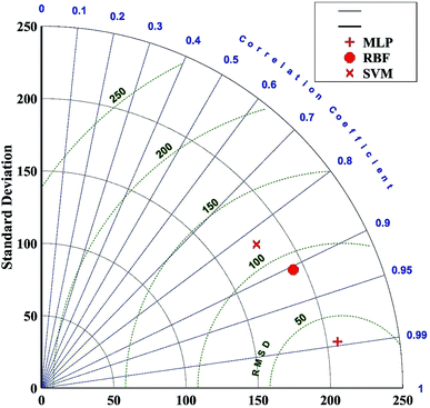
A Taylor diagram was also used to show the accuracy and efficiency of the models based on the observed values. The Taylor diagram provided a polar plot to summarize multiple aspects of the model and the observed parameters (i.e., correlation coefficient, normalized standard deviation and RMSD).46–48
We need to find the factors with the most effect on the model outputs to modify the diameter of the target nanofibers. Sensitivity analysis was performed on the final model to detect the importance of the variables concerning their role in the model outputs.
3 Results and discussion
3.1 Prediction performance of MLP
The electrospinning parameters (ratio blends of the polymer, applied voltage, injection rate and, the needle-to-collector distance), as input variables, and the effects of these parameters on the diameter of the PCL/gelatin nanofibers as outputs, were entered into the software MATLAB R2016b to design the most accurate prediction of the diameter for the nanofiber model (PDNFM)MLP. In the optimization of the MLP model parameters, the total number of samples (762 samples) was randomly divided into three data sets. The training data subset contained 60% of all samples (457 samples), the validation data set contained 20% of the samples (153 samples), and 20% of the samples (153 samples) were assigned to the test data to train, validate and test the PDNFMMLP. As we know, in the training method, to achieve the most accurate PDNFMMLP, the number of neurons and hidden layers, and the activation function should be optimized (Table 1).| Activation function | Training function | Structure | Test set | Training data | ||||||||
|---|---|---|---|---|---|---|---|---|---|---|---|---|
| R2 | MSE | RMSE | MAE | WI | R2 | MSE | RMSE | MAE | WI | |||
| logsig–logsig–purelin | LM | 4-10-10-1 | 0.96 | 0.036 | 0.19 | 0.097 | 0.9999984204 | 0.987 | 0.014 | 0.118 | 0.075 | 0.9999999967 |
We present the best activation function equations in the structure of the MLP model using eqn (14) and (15).
 | (14) |
| Purelin(x) = f(x) | (15) |
According to the values of R2 (Table 1), ANN optimization detected the structure of ‘4-10-10-1’ for PDNFMMLP as the most successful structure of MLP in the prediction of the diameter of PCL/Gt electrospinning nanofibers and effect of electrospinning parameters on the diameter of the PCL/gelatin nanofibers. The determined structure contains four variables as inputs, ten neurons in the two hidden layers, and one neuron (diameter of nanofibers) in the output layer. To use the most accurate estimation functions in the hidden layer and output layer, logarithmic sigmoid and linear transfer functions were used as a learning function, respectively.
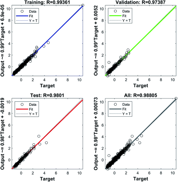
The scatter plot provides the correlation between variables which is used to define the accuracy of an ANN model.21,35 The scatter plot of the MLP outputs versus the target values of the PDNFMMLP for the training, validation, testing, and overall data sets are presented in Fig. 1. The determination of the coefficient (R2) proves the strong correlation between the PDNFMMLP outputs and the target values.
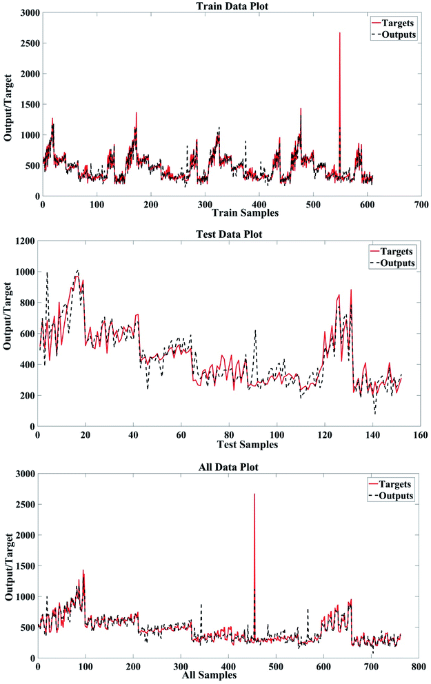
Fig. 2 compares the real (target) and simulated (output) values of PDNFMMLP in the data sets. A significant and distinctive agreement between values has been provided in Fig. 2.
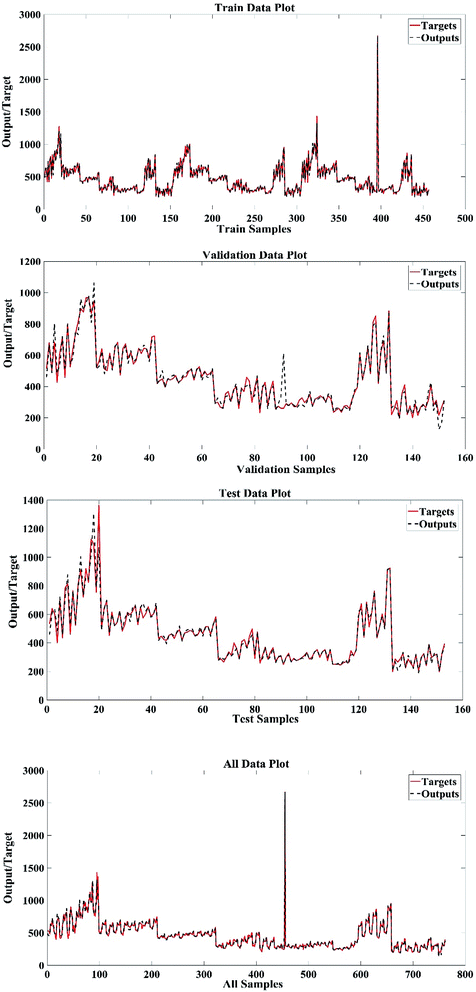 | ||
| Fig. 2 Target and output nanofiber diameter values for training, validation, and testing sets and all data. | ||
The PDNFMMLP, using four electrospinning parameters as model input variables, is the most accurate model for prediction of the diameter of electrospun PCL/Gt nanofibers against the changing electrospinning parameters. Eqn (16) is the logarithmic sigmoid and eqn (17) illustrates the PDNFMMLP in electrospun PCL/Gt nanofibers.
 | (16) |
| PDNFMMLP = purelin{logsig{∑LW2,1{logsig(∑IW1,1pi + b1)} + b2}} | (17) |
3.2 Prediction performance of RBFNN
In this type of ANN, the Gaussian transfer function is selected as the activation function in the hidden layer, which is the main difference from MLP. It consists of two layers: an input layer and an output layer to receive data for the training process. During the training process, the two main parameters that are optimized are the spread of the radial basis functions and the number of neurons.The electrospinning parameters (ratio blends of the polymer, applied voltage, injection rate and, the needle-to-collector distance), as input variables, and the diameter of the PCL/gelatin nanofibers as the outputs, were tagged in the software MATLAB R2016b. In model parameters optimization, 80% of samples (610 samples) were randomly defined as the training set to train the most accurate RBFNN, and 20% of samples (152 samples) were applied to test the performance of the PDNFMRBF. The aim of the training step was the network error minimization with RBFNN parameters values. Therefore, in the best PDNFMRBF performance, the number of neurons was 125, and the spread of the radial basis functions was 7. The best results for PDNFMRBF in the training and test data sets are shown in Table 2.
| Model | Spread | Neurons | Test set | Training data | ||||||||
|---|---|---|---|---|---|---|---|---|---|---|---|---|
| R2 | MSE | RMSE | MAE | WI | R2 | MSE | RMSE | MAE | WI | |||
| RBF | 7 | 125 | 0.821 | 0.136 | 0.368 | 0.269 | 0.9999907541 | 0.818 | 0.191 | 0.437 | 0.231 | 0.9999997597 |
As shown in Table 2, the optimal architecture is determined by the values of R2 in the training and test data sets. The best architecture of RBFNN was determined to be 4-125-1 with four variables as inputs, 125 neurons in the hidden layer with a Gaussian transfer function, and one neuron (diameter of nanofibers) in the output layer.
The scatter plot of the RBFNN outputs versus the target values of the PDNFMRBF for the training and test sets, and all data are presented in Fig. 3. The determination of the coefficient (R2) shows a significant correlation between the PDNFMRBF outputs and targets values.
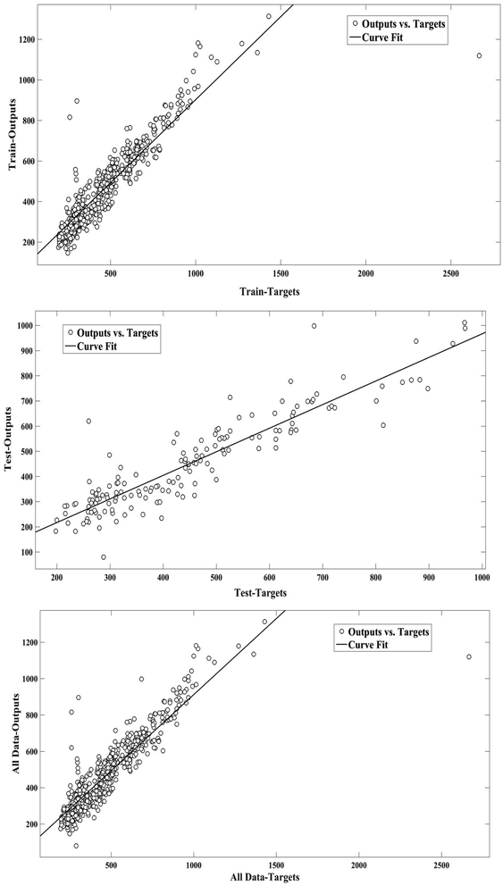 | ||
| Fig. 3 Scatter plots of PDNFMRBF outputs versus the target values for the training and test sets and all data. | ||
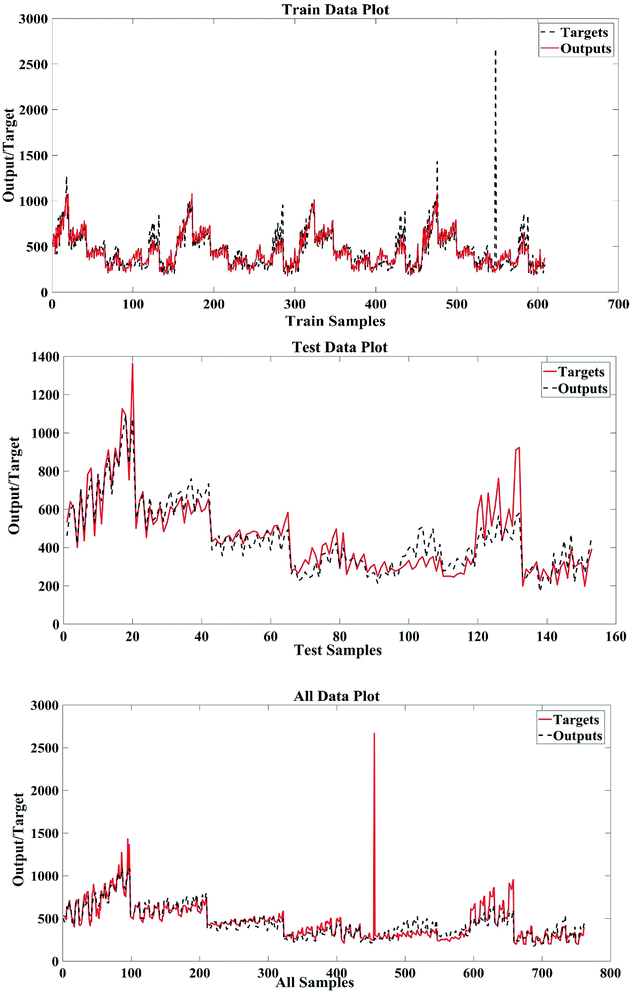
Fig. 4 compares the real (target) and simulated (output) values of PDNFMRBF in the data sets. A notable and satisfying agreement between the values can be observed in Fig. 4.
3.3 Prediction performance of SVM
As with other models, some parameters of SVM require optimization to improve the goal accuracy of the network. Usually, SVM employs some predefined functions, called kernels that can classify the data into a matrix with a multi-dimensional space that separates all data in this multi-dimensional space more easily.49,50The SVR regression performance is associated with the proper selection of the parameters, which are ε, C, and γ. The value of the ε is related directly to the number of support vectors.51 The value of γ is determined by the width of the bell-shaped curves in the structure of the SVM regression with a Gaussian function (as shown in eqn (7)). In this research, the polynomial kernel function was found to be more accurate than the Gaussian function; therefore, we did not achieve the value of γ. On the other hand, the value of C allows the SVM to gain more simple curves as the goal accuracy is obtained.42 Thus, we selected the values of the ε and C parameters to achieve a highly accurate SVM regression in the prediction of the diameter of the electrospun nanofibers. In the parameter optimization of PDNFMSVM, all data were divided into two subsets: 80% (610 samples) for the training network and 20% (152 samples) of data for testing the PDNFMSVM accuracy and generalization. Table 3 presents the most appropriate PDNFMSVM parameters and prediction accuracies for SVM regression of the train and test data.
| ε | C | Test set | Training data | ||||||||
|---|---|---|---|---|---|---|---|---|---|---|---|
| R2 | MSE | RMSE | MAE | WI | R2 | MSE | RMSE | MAE | WI | ||
| 62.02 | 888.78 | 0.829 | 0.0067 | 0.082 | 60 | 0.9991904256 | 0.657 | 0.0001 | 0.012 | 60.41 | 0.9987218987 |
The best finding was obtained for data modeling without data standardization, while the data was standardized in the MLP and RBFNN modeling to achieve better and faster findings. As shown in Table 3, the best ε value was 62.02, the C value was 887.78 concerning the values of R2 in the training and test data sets. Other models with other values of ε and C show over-fitting and under-fitting in models. In over-fitting models, a significantly higher R2 value is achieved in the training data set, but the accuracy of the PDNFMSVM is decreased significantly in the test data test. The PDNFMSVM is close to that of the training data, otherwise the model is over-trained. In under-fitting models, the performance of PDNFMSVM is not acceptable, or the best performance is not obtained.
The results obtained from the scatter plot of the SVM outputs versus the target values of the PDNFMSVM for the training and test sets, and all data are set out in Fig. 5. The determination of the coefficient (R2) shows the acceptable correlation between the PDNFMSVM outputs and the target values.
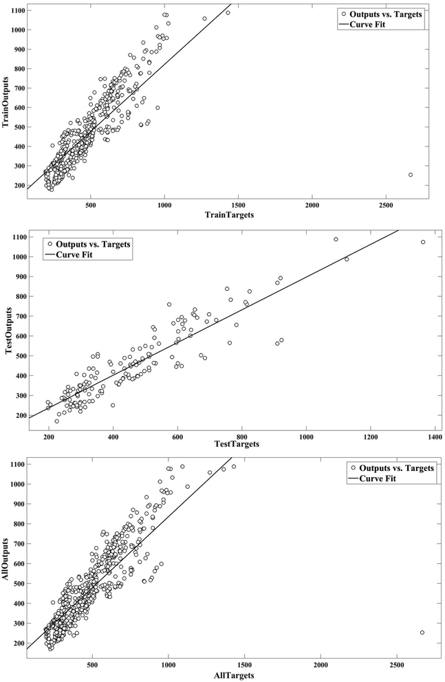 | ||
| Fig. 5 Scatter plots of PDNFMSVM outputs versus the target values for the training and test sets and for all data. | ||
Fig. 6 compares the real (target) and simulated (output) values of PDNFMSVM in the data sets. A notable and satisfying agreement between the values is observed in Fig. 6.
Fig. 7 provides the Taylor diagrams observed for the performances of the computing models (i.e., MLP, RBFF, and SVM). It is shown that the MLP model provided a higher RMSD and correlation coefficient compared to the RBFF and SVM models. Therefore, comparison of the findings of the models shows that the MLP is the most accurate model in the prediction of the diameter of the diameter of the PCL/Gt electrospun nanofibers (Fig. 7).
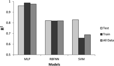
Comparing the findings of PDNFMMLP, PDNFMRBF, PDNFMSVM shows that PDNFMMLP is the most accurate model for the prediction of the diameter of the PCL/Gt electrospun nanofibers (Fig. 8). In comparison to RBFNN and SVM, the MLP model shows the highest R2 value in training, test, and total data sets. After randomizing the data, they were divided into training and test data sets so that the same training and test samples were used for the three modeling methods.
The properties and morphology of the electrospun nanofibers are critical factors when designing nanofibers for different applications. This property depends on many processing parameters.17,24 ANN models have been applied previously as a predictive modeling tool for electrospun nanofibers.52 For example, Ketabchi et al. developed and tested the accuracy of the ANN model for predicting the diameter of chitosan/PEO nanofibers in trials and studies and for analysis of the interactions between the involved electrospinning parameters and the diameter of the chitosan/PEO nanofibers with sufficient sensitivity and specificity.53 In this research, we attempted to validate the accuracy of data mining models such as MLP, RBFNN, and SVM, on the effects of processing parameters including the polymer weight ratios, nozzle–collector distance, applied voltage, and the injection rate on the average diameter of the electrospun PCL/Gt nanofibers.
As can be seen from Table 1, the MLP as an ANN modeling approach can successfully predict the structure of the PCL/Gt electrospun nanofibers with an accuracy of up to at least 0.96 (R2 in test data), so long as reliable and in range data are available to run the PDNFMMLP. Owing to the high degree of complexity in the relationships between the electrospinning parameters and the diameter of the nanofibers, these values were satisfactory.20 The successful application of a BP neural network and MLP in electrospinning studies has been proved in previously published research with a higher accuracy in comparison with the multiple regression models.31,54,55 The reliable results of ANN modeling in electrospinning nanofibers studies have been illustrated in previous studies in which Khanlou et al. aimed to employ an MLP network with a BP algorithm to assess the application of the ANN to predict and optimize the electrospinning parameters for polymethyl methacrylate nanofibers. Using an ANN with a three layer BP neural network, there is a perfect correlation between the targets and outputs. The correlation factors for the training and validation samples were 0.98 and 0.99, respectively.31 Another study showed the ability of an ANN to predict the diameter of polyurethane nanofibers by considering variables of the ratio of solvents, average molecular weight of polyurethane, concentration, voltage, distance, and the electric field. The results show that artificial neural networks can predict the diameter of electrospun polyurethane nanofibers well.56 In this research, PDNFMMLP provides a framework for accurate analyzing electrospinning parameters and the diameter of electrospun PCL/Gt nanofibers that will result in greater economy and save time. The results of the MLP approach, especially the greater accuracy (R2 = 0.96) obtained in comparison with the RBFNN (R2 = 0.821), and SVM (R2 = 0.829) results signify that PDNFMMLP can be used as a comparative impact assessment model for predicting the diameter of PCL/Gt nanofibers.
3.4 Sensitivity analysis of PDNFMMLP
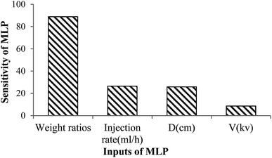
According to these results, PDNFMMLP show the best performance for the prediction of the diameter of PCL/Gt electrospun nanofibers. Thus, a sensitivity analysis of the predicted outputs of the optimal PDNFMMLP was conducted. In the sensitivity analysis, each parameter in the range of the standard deviation with 50 steps were changed, while the other parameters were fixed at the value of the average. Next, the standard deviation of the outputs for each parameter change were measured as the PDNFMMLP sensitivity for that parameter. As illustrated in Fig. 9, the PDNFMMLP sensitivities for the input variables have been explored using sensitivity analysis. The results of the sensitivity analysis demonstrate that the electrospinning processing parameters play a primary role in the MLP outputs. As can be seen from Fig. 9, the value of the PCL/Gt weight ratios is detected as the most significant input influencing the PDNFMMLP output.Fig. 10a and c shows the effect of the PCL/Gt weight ratios and applied voltage on the diameter of the fiber. As one can see, there is a negative correlation between the weight ratio and the voltage and fiber diameter, therefore the fiber diameter decreases with the increased voltage or weight ratios. The fiber diameter decreased upon increasing the content of PCL in the AA/FA solution, as shown in Fig. 10a. A reason for this result could be the presence of an emulsion, which can be weakened at higher PCL contents. PCL/Gt exhibit an emulsion structure when using an AA or AA/FA mixture as a solvent. The explanation for this emulsion structure is the absence, or very limited miscibility, of Gt and PCL and the relatively weak interaction with AA and FA. These results are in accordance with those obtained by Denis et al.29 Also, a decrease in the viscosity of the polymer solution can be ascribed as the cause of the decrease in the nanofiber diameter.57 As shown in Fig. 10b, the effect of distance on the diameter of the nanofiber is contradictory, the fiber diameter increases, as well as decreases, with an increase of the distance. Indeed, at a short spinning distance, there will not be sufficient time for the solvent to evaporate before the jet is placed on the collector owing to thicker nanofibers. Furthermore, the diameter of the nanofibers decreased with an increase in the spinning distance.58 The curve is downward-sloping for high values of the spinning distance. This result may be explained by the fact that by increasing the spinning distance, the jet has enough time to stretch and the solvent will have more time to evaporate before the jet is deposited on the collector leading to thinner fiber formation.58 Another reason is probably owing to breaking of the formed jet into two or more jets, leading to finer nanofibers.20 These results were reported in recent studies.56–58 Fig. 10c shows the effect of applied voltage on the diameter of the nanofibers. In fact, at a high applied voltage, the electric field strength is high, resulting in further stretching of the jet before it is deposited on the collector, and hence the fiber diameter will decrease. On the other hand, increasing the applied voltage will result in an increased surface charge on the droplet jet, favoring the formation of thinner fibers. This observation is in agreement with those from previously published reports.59–61
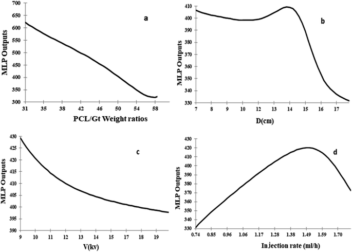 | ||
| Fig. 10 The trend of the DPNFMMLP output changes upon varying: the (a) PCL/Gt weight ratio; (b) distance; (c) voltage; and (d) injection rate. | ||
Considering the trends observed in Fig. 10d, the injection rate has a two-fold impact on the diameter of the fiber. First, the diameter of the nanofibers increases with an increase in the volume injection rate. The published literature indicates that an increase in the injection rate of the solution typically increases the diameter of the nanofibers.62,63 This result could be explained by the fact that an increase in injection rate leads to an increase of the amount of polymer solution delivered to the top of the needle making the jet diameter increase.57,58,62 Therefore there is a limitation to this, after reaching an optimum value, the diameter of the nanofibers continuously decrease with an increase in the injection rate. Some studies show that the injection rate increase leads to a decrease in the diameter of the nanofibers.20,64 As increasing the injection rate will cause higher electrostatic forces, an increase in the volumetric charge density on the droplet jet, and a greater tensile force which might increase the stretching of the jet, resulting in the formation of thinner diameter nanofibers.59,65 The literature shows that ANN techniques have been designed with data analysis, modeling, simulation, and output.21 These models have been used to investigate the relationship between electrospinning parameter and the diameter of the nanofibers or fiber morphology .1,58
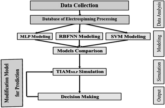
PDNFMMLP provides a new tool as a prediction model for the electrospinning of nanofiber considering the variables of the PCL/Gt weight ratios, applied voltage, distance and, injection rate. PDNFMMLP provides a new tool as a DSS in PCL/Gt electrospinning for prediction of the diameter of the nanofibers resulting from electrospinning. PDNFMMLP was developed for researchers or lab technician to predict the diameter of PCL/Gt nanofibers, which helps them to save time and money. In this study, which develops a tool for the prediction of the diameter of PCL/Gt nanofibers, the steps of model development and implementation are described as a DSS. We proposed the flow diagram shown in Fig. 11 to design a DSS using PDNFMMLP for PCL/Gt electrospinning. The described DSS has been designed using data analysis, modeling, simulation, and output. The output of PDNFMMLP is applicable in the electrospinning of PCL/Gt nanofibers, and the electrospinning processing parameters and diameter of PCL/Gt nanofibers could be modified based on the proposed DSS to reduce time and costs. The values of the optimization factors are not proposed for use in other research, but they could be used as alternatives values to optimize models in this kind of research. Finally, a graphical user interface (GUI) was designed to run the PDNFM model on new data for which the researchers are planning for PCL/Gt electrospinning. A GUI, as a user friendly tool, is designed to provide easy utilization of an ANN technique. The GUI provides a tool to predict nanofiber diameter before electrospinning by changing the values of the input parameters, which saves time and material.66
In general, it is necessary to mention that sizes at the nanoscale significantly impact the structural, mechanical, thermal, thermo-dynamic, kinetic, and electrical properties of materials.28 Furthermore, rapidly increasing interest has been shown by users, and this has led to the production of diverse nanofibers for versatile usage in various applications.67 Determination of the nanofiber size is, therefore, a matter of considerable importance in electrospinning for various applications.68 With the help of the PDNFM model, the changes are detectable before electrospinning. This means that a change in the diameter of the nanofibers and the morphology is measurable before electrospinning. The researchers, engineers, and experts working in academia and industry can easily predict the diameter of nanofibers in electrospinning. GUI as a DSS tool will be run on new data by simply inputting the diameter of the nanofiber, as shown in Fig. 12. As an example, Fig. 12 illustrates the effect of two different electrospinning processing parameters on the diameter of PCL/Gt nanofibers. We found the diameter of nanofibers to be thick (200 to 500 nm) in plan (a) for our specific application in PCL/Gt electrospinning. Therefore, we modified the electrospinning processing parameters of plan (a) to plan (b), in which the diameter of the nanofibers will be optimal in PCL/Gt electrospinning for our application. The modification was conducted by changing the most significant factors in the sensitivity analysis results and trends shown in Fig. 10. Overall, the findings of this study indicate the advantages of modeling and optimizing the diameter of electrospun nanofibers using an ANN and the advantages of these models for experts in the nano-field, tissue engineering, pharmaceutical, environmental, medical, food and engineering industries to help reduce product costs.
4 Conclusions
In this research, MLP, RBFNN, and SVM models were developed to predict the diameter of a PCL/Gt nanofiber considering variables such as the PCL/Gt weight ratios, applied voltage, distance, and injection rate. The performance of the designed MLP, RBFNN, and SVM models was evaluated by root mean squared error, mean absolute error, coefficient of determination, Willmott's index, and a Taylor diagram. Furthermore, the sensitivity for each electrospinning parameter has been explored using sensitivity analysis. In the structure provided using MATLAB software, the results indicated the greater accuracy of the MLP compared with the RBFF and SVM models and showed the potential of the MLP modeling technique as a handy tool for predicting the ideal electrospinning process parameters and nanofiber properties. It also showed that the PCL/Gt weight ratio is the most significant input which influences the MLP output. It is recommended to apply a modeling approach such as the MLP model to estimate and optimize the size of nanofibers before electrospinning. This can be worthwhile in terms of the economy, time, and scientific aims. It can thus be suggested that designing and applying the prediction method for different kind of nanofibers or nanomaterials should be performed using ANN techniques for various applications in environmental, medical and other industries.Conflicts of interest
There are no conflicts to declare.Acknowledgements
The authors would like to acknowledge the Tehran University of Medical Sciences and the College of Environment.Notes and references
- K. Nasouri, Novel estimation of morphological behavior of electrospun nanofibers with artificial intelligence system (AIS), Polym. Test., 2018, 69, 499–507 CrossRef CAS.
- M. Naghibzadeh and M. Adabi, Evaluation of effective electrospinning parameters controlling gelatin nanofibers diameter via modelling artificial neural networks, Fibers Polym., 2014, 15(4), 767–777 CrossRef CAS.
- B. Feng, S. Wang, D. Hu, W. Fu, J. Wu and H. Hong, et al., Bioresorbable electrospun gelatin/poly(ε-caprolactone) nanofibrous membrane as a barrier to prevent cardiac postoperative adhesion, Acta Biomater., 2019, 83, 211–220 CrossRef CAS PubMed.
- W. P. Lu and Y. Guo, Electrospinning of Collagen and Its Derivatives for Biomedical Applications, Novel Aspects of Nanofibers, IntechOpen, 2018 Search PubMed.
- M. E. Hoque, T. Nuge, T. Yeow and N. Nordin, Electrospinning of gelatin nanofibre: current trends in tissue engineering applications, J. Appl. Mech. Eng., 2013, 2, e122 Search PubMed.
- L. Ghasemi-Mobarakeh, M. P. Prabhakaran, M. Morshed, M.-H. Nasr-Esfahani and S. Ramakrishna, Electrospun poly(ε-caprolactone)/gelatin nanofibrous scaffolds for nerve tissue engineering, Biomaterials, 2008, 29(34), 4532–4539 CrossRef CAS PubMed.
- L. Van der Schueren, B. De Schoenmaker, Ö. I. Kalaoglu and K. De Clerck, An alternative solvent system for the steady state electrospinning of polycaprolactone, Eur. Polym. J., 2011, 47(6), 1256–1263 CrossRef CAS.
- Y. H. Wu, D. G. Yu, H. P. Li, X. Y. Wu and X. Y. Li, Medicated structural PVP/PEG composites fabricated using coaxial electrospinning, e-Polym., 2017, 17(1), 39–44 CAS.
- Q. Wang, D. G. Yu, L. L. Zhang, X. K. Liu, Y. C. Deng and M. Zhao, Electrospun hypromellose-based hydrophilic composites for rapid dissolution of poorly water-soluble drug, Carbohydr. Polym., 2017, 174, 617–625 CrossRef CAS PubMed.
- C. Yang, D. G. Yu, D. Pan, X. K. Liu, X. Wang, S. A. Bligh and G. R. Williams, Electrospun pH-sensitive core–shell polymer nanocomposites fabricated using a tri-axial process, Acta Biomater., 2016, 35, 77–86 CrossRef CAS PubMed.
- K. Wang, X. K. Liu, X. H. Chen, D. G. Yu, Y. Y. Yang and P. Liu, Electrospun hydrophilic Janus nanocomposites for the rapid onset of therapeutic action of helicid, ACS Appl. Mater. Interfaces, 2018, 10(3), 2859–2867 CrossRef CAS PubMed.
- D. G. Yu, J. J. Li, M. Zhang and G. R. Williams, High-quality Janus nanofibers prepared using three-fluid electrospinning, Chem. Commun., 2017, 53(33), 4542–4545 RSC.
- M. Naghibzadeh, M. Adabi, H. R. Rahmani, M. Mirali and M. Adabi, Evaluation of the effective forcespinning parameters controlling polyvinyl alcohol nanofibers diameter using artificial neural network, Adv. Polym. Technol., 2018, 37(6), 1608–1617 CrossRef CAS.
- W. Huang, Y. Hou, X. Lu, Z. Gong, Y. Yang, X. J. Lu, X. L. Liu and D. G. Yu, The Process–Property–Performance Relationship of Medicated Nanoparticles Prepared by Modified Coaxial Electrospraying, Pharmaceutics, 2019, 11(5), 226 CrossRef PubMed.
- X. Wang, L. Zhao, J. Y. Fuh and H. P. Lee, Effect of Porosity on Mechanical Properties of 3D Printed Polymers: Experiments and Micromechanical Modeling Based on X-Ray Computed Tomography Analysis, Polymers, 2019, 11(7), 1154 CrossRef CAS PubMed.
- H. Zhou, Z. Shi, X. Wan, H. Fang, D. G. Yu, X. Chen and P. Liu, The Relationships between Process Parameters and Polymeric Nanofibers Fabricated Using a Modified Coaxial Electrospinning, Nanomaterials, 2019, 9(6), 843 CrossRef CAS PubMed.
- B. H. Moghadam, M. Hasanzadeh and A. Haghi, On the contact angle of electrospun polyacrylonitrile nanofiber mat, Bulg. Chem. Commun., 2013, 45, 169–177 CAS.
- M. D. Chomachayi, A. Solouk and H. Mirzadeh, Electrospun silk-based nanofibrous scaffolds: fiber diameter and oxygen transfer, Prog. Biomater., 2016, 5(1), 71–80 CrossRef CAS PubMed.
- S. Rafiei, S. Maghsoodloo, B. Noroozi, V. Mottaghitalab and A. Haghi, Mathematical modeling in electrospinning process of nanofibers: a detailed review, Cellul. Chem. Technol., 2013, 47, 323–338 CAS.
- R. Faridi-Majidi, H. Ziyadi, N. Naderi and A. Amani, Use of artificial neural networks to determine parameters controlling the nanofibers diameter in electrospinning of nylon-6,6, J. Appl. Polym. Sci., 2012, 124(2), 1589–1597 CrossRef CAS.
- A. Jahani, Forest landscape aesthetic quality model (FLAQM): a comparative study on landscape modelling using regression analysis and artificial neural networks, J. For. Sci., 2019, 65(2), 61–69 CrossRef.
- S. Akbarifard and F. Radmanesh, Predicting sea wave height using Symbiotic Organisms Search (SOS) algorithm, Ocean Eng., 2018, 167, 348–356 CrossRef.
- H. Aghajani, M. M. Mohadjer, A. Jahani, M. R. Asef, A. Shirvany and M. Azaryan, Investigation of affective habitat factors affecting on abundance of wood macrofungi and sensitivity analysis using the artificial neural network (case study: Kheyrud forest, Noshahr), Iranian Journal of Forest and Poplar Research, 2014, 21(4), 617–627 Search PubMed.
- E. Vatankhah, D. Semnani, M. P. Prabhakaran, M. Tadayon, S. Razavi and S. Ramakrishna, Artificial neural network for modeling the elastic modulus of electrospun polycaprolactone/gelatin scaffolds, Acta Biomater., 2014, 10(2), 709–721 CrossRef CAS PubMed.
- K. Qaderi, S. Akbarifard, M. R. Madadi and B. Bakhtiari, Optimal operation of multi-reservoirs by water cycle algorithm, Proceedings of the Institution of Civil Engineers - Water Management, 2017, 171(4), 179–190 CrossRef.
- A. Jahani, J. Feghhi, M. F. Makhdoum and M. Omid, Optimized forest degradation model (OFDM): an environmental decision support system for environmental impact assessment using an artificial neural network, J. Environ. Plan. Manag., 2016, 59(2), 222–244 CrossRef.
- A. Rabbi, K. Nasouri, H. Bahrambeygi, A. M. Shoushtari and M. R. Babaei, RSM and ANN approaches for modeling and optimizing of electrospun polyurethane nanofibers morphology, Fibers Polym., 2012, 13(8), 1007–1014 CrossRef CAS.
- A. Jahani, Aesthetic quality evaluation modeling of forest landscape using artificial neural network, Wood & Forest Science and Technology, 2017, 24(3), 17–22 Search PubMed.
- P. Denis, J. Dulnik and P. Sajkiewicz, Electrospinning and structure of bicomponent polycaprolactone/gelatin nanofibers obtained using alternative solvent system, Int. J. Polym. Mater. Polym. Biomater., 2015, 64(7), 354–364 CrossRef CAS.
- J. Dulnik, P. Denis, P. Sajkiewicz, D. Kołbuk and E. Choińska, Biodegradation of bicomponent PCL/gelatin and PCL/collagen nanofibers electrospun from alternative solvent system, Polym. Degrad. Stab., 2016, 130, 10–21 CrossRef CAS.
- H. M. Khanlou, A. Sadollah, B. C. Ang, J. H. Kim, S. Talebian and A. Ghadimi, Prediction and optimization of electrospinning parameters for polymethyl methacrylate nanofiber fabrication using response surface methodology and artificial neural networks, Neural Comput. Appl., 2014, 25(3–4), 767–777 CrossRef.
- B. T. Pham, M. D. Nguyen, K.-T. T. Bui, I. Prakash, K. Chapi and D. T. Bui, A novel artificial intelligence approach based on multi-layer perceptron neural network and biogeography-based optimization for predicting coefficient of consolidation of soil, Catena, 2019, 173, 302–311 CrossRef.
- A. Jahani, Modeling of forest canopy density confusion in environmental assessment using artificial neural network, Iranian Journal of Forest and Poplar Research, 2016, 24(2), 310–321 Search PubMed.
- A. Jahani and F. A. Mohammadi, Aesthetic quality modeling of landscape in urban green space using artificial neural network, Journal of Natural Environment, 2017, 69(4), 951–963 Search PubMed.
- A. Jahani, Sycamore failure hazard classification model (SFHCM): an environmental decision support system (EDSS) in urban green spaces, Int. J. Environ. Sci. Technol., 2019, 16(2), 955–964 CrossRef.
- S. Shafiee and S. Minaei, Combined data mining/NIR spectroscopy for purity assessment of lime juice, Infrared Phys. Technol., 2018, 91, 193–199 CrossRef CAS.
- Q. He, H. Shahabi, A. Shirzadi, S. Li, W. Chen and N. Wang, et al., Landslide spatial modelling using novel bivariate statistical based Naïve Bayes, RBF Classifier, and RBF Network machine learning algorithms, Sci. Total Environ., 2019, 663, 1–15 CrossRef CAS PubMed.
- Y. Yao, L. Dai, F. Jiang, W. Liao, M. Dong and X. Yang, Kinetic modeling of novel solid desiccant based on PVA-LiCl electrospun nanofibrous membrane, Polym. Test., 2017, 64, 183–193 CrossRef CAS.
- W. Lü, Y. Chen, W. Ma, X. Zhang, F. Luan and M. Liu, et al., QSAR study of neuraminidase inhibitors based on heuristic method and radial basis function network, Eur. J. Med. Chem., 2008, 43(3), 569–576 CrossRef PubMed.
- N. Qu, X. Li, Y. Dou, H. Mi, Y. Guo and Y. Ren, Nondestructive quantitative analysis of erythromycin ethylsuccinate powder drug via short-wave near-infrared spectroscopy combined with radial basis function neural networks, Eur. J. Pharm. Sci., 2007, 31(3–4), 156–164 CrossRef CAS PubMed.
- L. Wang, Support vector machines: theory and applications, Springer Science & Business Media, 2005 Search PubMed.
- W.-H. Chen, S.-H. Hsu and H.-P. Shen, Application of SVM and ANN for intrusion detection, Comput. Oper. Res., 2005, 32(10), 2617–2634 CrossRef.
- A. Jahani, Sycamore failure hazard risk modeling in urban green space, Journal of Spatial Analysis Environmental Hazards, 2017, 3(4), 35–48 CrossRef.
- S. Akbarifard and B. Bakhtiari, Optimal allocation of water resources using Water Cycle Algorithm (WCA) (Case study: Gorganrood basin), Water Engineering, 2018, 11(36), 33–46 Search PubMed.
- S. Rezazadeh, A. Jahani, M. Makhdoum and H. G. Meigooni, Evaluation of the Strategic Factors of the Management of Protected Areas Using SWOT Analysis—Case Study: Bashgol Protected Area-Qazvin Province, Open J. Ecol., 2017, 7(01), 55–68 CrossRef.
- R. Khatibi, M. A. Ghorbani and F. A. Pourhosseini, Stream flow predictions using nature-inspired Firefly Algorithms and a Multiple Model strategy – Directions of innovation towards next generation practices, Adv. Eng. Inf., 2017, 34, 80–89 CrossRef.
- M. A. Ghorbani, R. C. Deo, Z. M. Yaseen, M. H. Kashani and B. Mohammadi, Pan evaporation prediction using a hybrid multilayer perceptron-firefly algorithm (MLP-FFA) model: case study in North Iran, Theor. Appl. Climatol., 2018, 133(3–4), 1119–1131 CrossRef.
- S. Kim, Y. Seo, M. Rezaie-Balf, O. Kisi, M. A. Ghorbani and V. P. Singh, Evaluation of daily solar radiation flux using soft computing approaches based on different meteorological information: peninsula vs. continent, Theor. Appl. Climatol., 2018, 137(1–2), 1–20 Search PubMed.
- S. Niell, F. Jesús, R. Díaz, Y. Mendoza, G. Notte and E. Santos, et al., Beehives biomonitor pesticides in agroecosystems: Simple chemical and biological indicators evaluation using Support Vector Machines (SVM), Ecol. Indicat., 2018, 91, 149–154 CrossRef CAS.
- F. Tourlomousis and R. C. Chang, Dimensional metrology of cell-matrix interactions in 3D microscale fibrous substrates, Procedia CIRP, 2017, 65, 32–37 CrossRef.
- R. Laref, E. Losson, A. Sava and M. Siadat, On the optimization of the support vector machine regression hyperparameters setting for gas sensors array applications, Chemom. Intell. Lab. Syst., 2019, 184, 22–27 CrossRef CAS.
- M. M. Abolhasani, K. Shirvanimoghaddam, H. Khayyam, S. M. Moosavi, N. Zohdi and M. Naebe, Towards predicting the piezoelectricity and physiochemical properties of the electrospun P(VDF-TrFE) nanogenerators using an artificial neural network, Polym. Test., 2018, 66, 178–188 CrossRef CAS.
- N. Ketabchi, M. Naghibzadeh, M. Adabi, S. S. Esnaashari and R. Faridi-Majidi, Preparation and optimization of chitosan/polyethylene oxide nanofiber diameter using artificial neural networks, Neural Comput. Appl., 2017, 28(11), 3131–3143 CrossRef.
- T. Khatti, H. Naderi-Manesh and S. M. Kalantar, Application of ANN and RSM techniques for modeling electrospinning process of polycaprolactone, Neural Comput. Appl., 2019, 31(1), 239–248 CrossRef.
- Neural network modeling of smart nanostructure sensor for electronic nose application, 6th International Conference on Systems and Control (ICSC), ed. S. Khaldi and Z. Dibi, Batna, Algeria, 2017 Search PubMed.
- E. Hosaini-Alvand, H. Mirshekar, M. Taghi Khorasani, M. Parvazinia and A. Joorabloo, Fabricating and robust artificial neural network modeling nanoscale polyurethane fiber using electrospinning method, J. Appl. Polym. Sci., 2017, 134(30), 45116 CrossRef.
- S. Baghersad, S. H. Bahrami, M. R. Mohammadi, M. R. M. Mojtahedi and P. B. Milan, Development of biodegradable electrospun gelatin/aloe-vera/poly(ε-caprolactone) hybrid nanofibrous scaffold for application as skin substitutes, Mater. Sci. Eng. C, 2018, 93, 367–379 CrossRef CAS.
- D. Nurwaha, W. Han and X. Wang, Effects of processing parameters on electrospun fiber morphology, J. Text. Inst., 2013, 104(4), 419–425 CrossRef.
- C. Thompson, G. G. Chase, A. Yarin and D. Reneker, Effects of parameters on nanofiber diameter determined from electrospinning model, Polymer, 2007, 48(23), 6913–6922 CrossRef CAS.
- S. Theron, E. Zussman and A. Yarin, Experimental investigation of the governing parameters in the electrospinning of polymer solutions, Polymer, 2004, 45(6), 2017–2030 CrossRef CAS.
- A. Haghi, Electrospun nanofibers research: Recent developments, Nova Science Publishers Incorporated, 2009 Search PubMed.
- M. Costolo, J. Lennhoff, R. Pawle, E. Rietman and A. Stevens, A nonlinear system model for electrospinning sub-100 nm polyacrylonitrile fibres, Nanotechnology, 2007, 19(3), 035707 CrossRef PubMed.
- Q. Shao, R. C. Rowe and P. York, Comparison of neurofuzzy logic and neural networks in modelling experimental data of an immediate release tablet formulation, Eur. J. Pharm. Sci., 2006, 28(5), 394–404 CrossRef CAS PubMed.
- S. Ramakrishna, An introduction to electrospinning and nanofibers, World Scientific, 2005 Search PubMed.
- T. Wu, X. Chen, J. Sha, Y.-Y. Peng, Y.-L. Ma and L.-S. Xie, et al., Fabrication of shish-kebab-structured carbon nanotube/poly(ε-caprolactone) composite nanofibers for potential tissue engineering applications, Rare Met., 2019, 38(1), 64–72 CrossRef CAS.
- G. G. Ahmad, Using artificial neural networks with graphical user interface to predict the strength of carded cotton yarns, J. Text. Inst., 2016, 107(3), 386–394 CrossRef CAS.
- F. A. Paskiabi, E. Mirzaei, A. Amani, M. A. Shokrgozar, R. Saber and R. Faridi-Majidi, Optimizing parameters on alignment of PCL/PGA nanofibrous scaffold: An artificial neural networks approach, Int. J. Biol. Macromol., 2015, 81, 1089–1097 CrossRef CAS PubMed.
- S. S. Esnaashari, M. Naghibzadeh, M. Adabi and R. Faridi Majidi, Evaluation of the Effective Electrospinning Parameters Controlling Kefiran Nanofibers Diameter Using Modelling Artificial Neural Networks, Nanomed. Res. J., 2017, 2(4), 2239–2349 Search PubMed.
| This journal is © The Royal Society of Chemistry 2019 |

