A matching algorithm with isotope distribution pattern in LC-MS based on support vector machine (SVM) learning model

Abstract

In proteomics, it is important to detect, analyze, and quantify complex peptide components and differences. The key is to match the elution time peaks (LC peaks) produced by the same peptide in replicate experiments. Warping functions are currently widely used to correct the mean of time shifts among replicates. However, they cannot reduce the ambiguity to distinguish the corresponding peak pairs and the non-corresponding ones because the time shifts are random based on each extracted-ion-chromatogram (XIC). In this paper, besides time feature, isotope distribution pattern similarity is considered. The novelty is that compared with other feature based methods including the isotope feature, the algorithm is not based on the peak profile similarity as usual, but on the isotope distribution similarity. First, the training set of peptides including the corresponding and non-corresponding peak pairs were selected from the MS/MS results. Second, we generated time difference and isotope distribution pattern similarities for each peak pair. Third, Support Vector Machine (SVM) classification was used based on the two features. Finally, the accuracy was measured along with final coverage. We first used a 10-fold cross validation to test the effectiveness of the SVM learning model. The accuracy of correct matching could reach 97%. Second, we evaluated the coverage based on the learning model, which could be from 75% to 91% in different datasets. Thus, this matching algorithm based on time and isotope distribution pattern features could provide a high accuracy and coverage for the corresponding peak identification.

---

1 Introduction

Liquid chromatography-mass spectrometry/tandem mass spectrometry (LC-MS/MS) is a powerful tool for protein identification and quantification.¹ Replicates can improve its accuracy – these spectra should be the same. Theoretically, each experimental results should contain the same peptide compositions, and the peaks of a specific peptide in different spectral results should have the same LC time and m/z value. However, various uncontrollable factors lead to differences between the experimental results. Most of the popular approaches align the time shift first and then find the corresponding peaks. Most of the alignment approaches use warping functions² that correct the mean of the elution time shifts between the different datasets. Correlation optimized warping was proposed by Nielsen³ to which Bylund later proposed many modifications.^4,5 Parametric time warping (PTW) was proposed by Eilers,⁶ based on which Van developed an extension called semi-parametric time warping (STW).⁷ Wehrens described a new formulation based on PTW. Prince⁸ proposed an Obi-Warp by generating a warping function based on dynamic time warping with a one-to-one smooth warp function. Tomasz⁹ proposed a method for classification with the nearest neighbor rule, which combined the dynamic time warping (DTW) distance between multivariate time series (MTS) and the DTW distance between derivatives of MTS. These worked on peak-picked features rather than on complete profiles.¹⁰

The feature-based approaches mainly focus on either matching LC peaks or significant features in images.^11,12 Jaitly¹³ proposed a very sophisticated algorithm called LCMSWARP and compared six freely available alignment algorithms. OpenMS¹⁴ performed the best on proteomics data, closely followed by XAlign, XCMS and MZmine. For the metabolomics data sets, XCMS performed best with OpenMS not far behind. Voss's paper¹⁵ focused on the alignment of multiple datasets at the same time, in which the method combined hierarchical pairwise correspondence estimation and global retention time correction. However, the performance was slightly worse than OpenMS on proteomics data. In addition, some popular software package such as OpenMS^16,17 or msInspect^18,19 could align and match the peptides that were identified by the tandem MS; this generated low quantification coverage.²⁰ MaxQuant^21,22 looked for the LC elution peaks of all the identified peptides in LC/MS to ensure that the identified peptides from MS/MS could be quantified at least once.²³ However, if the peptide was identified in dataset 1 and not in dataset 2, then it was hard to quantify the corresponding peak in dataset 2.

As mentioned above, most matching algorithms processed the data via MS/MS. This could lead to accurate peptide information including m/z and LC time value. However, the XICs generated based on the MS/MS information have crowed peaks (Fig. 1)

Fig. 1 Interference of peptide “AGGPTTPLSPTR”. (a) The LC peak between 2800–3400 of peptide “AGGPTTPLSPTR” in data 1. (b) The LC peak between 2800–3400 of peptide “AGGPTTPLSPTR” in data 2.

Even after using the warping function to correct for the mean time difference, there still were ambiguous multiple LC peaks within a narrow time window. For example, it was difficult to identify which peak was the corresponding one for peptide “AGGPTTPLSPTR” in data 1 based on the real peak information in data 2. Time was still an important key for aligning, but there were some ambiguous peaks that could interrupt the correct matching. A unique statistical corresponding feature identification algorithm (SCFIA) was proposed in by Cui,²⁴ which used peak shape correlation between two peaks as an additional feature for matching. The peak shape correlation feature was directly calculated based on peak shapes. Another algorithm named PeakLink (PL) was proposed by Bari,²⁵ which used wavelet decomposition to reduce noise and calculated peak shape correlation scores after de-noising, and used the support vector machine (SVM) based on time and peak shape feature. The accuracy could achieve almost 90% with 5–8% improvement compared with SCFIA. These two methods proved that beside LC time, the additional feature could improve the aligning and matching accuracy. However, the selection of the second feature was crucial. As observed from the experiment result, the peak shape were affected by both signal and noise. If the peak shape was affected only by white noise, the wavelet decomposition could effectively remove it, because the statistical characteristics of white noise had not been changed after wavelet decomposition. However the composition of noise was complex, which affected the peak shape seriously.

At present, the analytical techniques of stable isotopes such as ¹³C, ¹⁸O and ¹⁵N were widely used in the biological field, because the isotope of peptide followed the same distribution. A computational platform entitled MetSign was proposed by Wei,²⁶ in which peak list alignment was based on isotope peaks. It also applied wavelet transformation (WT) for noise removal in order to get isolated peak profiles. MetSign performed peak alignment based on peak m/z values and the peak intensity profile of peaks.

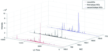
So till now, these feature based methods including the isotope feature were all based on the peak profile similarity, not on the distribution. The common way they used was calculating Pearson correlation coefficient to measure the similarity between the peaks. In this paper, compared with the peak intensity profile, the isotope distribution pattern was selected as the second feature, of which the characteristics of distribution of the peptide XICs were analyzed. The main (monoXICs), the first and second isotopes XICs should be very stable in the total distribution. Fig. 2 was the example of the peptide “ACNLDVILGFDGSR”.

Fig. 2 The isotope XICs of peptide “ACNLDVILGFDGSR”.

The SVM learning model was applied to align the peaks of the same peptide in different datasets via time features and also isotope distribution pattern similarity. The model would judge whether they correspond or not after calculation of time differences and isotope distribution pattern similarities. Taking two datasets as example in Fig. 3, there were 1944 peptides in dataset 1 and 1603 in dataset 2 detected by MS/MS. Fig. 3 showed that the intersection part (zone 2) had only 700 peptides; each peptide had the real LC time and m/z value information. These were selected as the total training candidate peptide set to build and test the SVM classification model. The final goal of this paper was to align and match all the peptides in zone 1 and zone 3 as well as possible.

Fig. 3 Venn diagram of two datasets with MS/MS information in Group 1.

2 Data and methods

2.1 Data

The datasets processed here were produced by RCMI Proteomics and Protein Biomarkers Cores at UTSA Laboratory. We totally used 3 groups of datasets. The X!Tandem in Trans-Proteomic Pipeline (TPP) was used to process all the datasets for tandem MS identification. The MS/MS list of each dataset contained peptide information, charge state, LC time value, intensity value and so on.

Group 1 contained two replicates of TAGE tumor datasets processed from the LTQ Orbitrap Velos instrument, which had already shown in Fig. 3. The dataset 1 contained 1944 peptide detected by MS/MS while the data 2 had 1603. The intersection had 700 peptides.

Group 2 contained the data from three fractions of breast cancer tissue together with a super-SILAC mix collected on an Orbitrap instrument. There were 6552, 6383, 4156 peptides detected by MS/MS in data 1, data 2 and data 3. The intersection of data 1 and 2 contained 1697, while 906 for data 1 and 3; 2409 for data 2 and 3. The intersection of the three datasets had 795 peptides.

Group 3 contained three technical replicates without prior separation collected on a new generation LTQ-Orbitrap Velos instrument. The number of peptides detected by MS/MS in data 1, 2 and 3 are 6207, 5892 and 6502. There were 4187 peptides in the intersection between data 1 and 2, while 4355 between data 1 and 3, 4287 between data 2 and 3. The intersection of these three datasets contained 3467 peptides.

These data groups were representative of real biological datasets collected on different instruments, each of which contained hundreds of thousands of isotopically labeled peptides.

2.2 Methods

The algorithm was developed by Matlab R2016a with SVM classification toolbox. The computer used for processing contained CPU i7-8700, 16 G RAM, 2T HDD and so on. Fig. 4 showed that the algorithm contained four parts: data preprocessing, generating total training candidate set, model building and testing, and full-scale alignment and matching.

Fig. 4 Flowgram of algorithm.

2.2.1 Data preprocessing. First, the two MS/MS datasets were combined to get unified peptide information. Second, based on the information list, we calculated the m/z value for the peptide as the center m/z value and generated the full-time XICs of mono-isotope, first isotope and second isotope for each peptide with a 20 ppm width window. Third, we detected the LC intervals in each XIC of the peptide. Finally, peptides with the intervals that contained the MS/MS time information were selected. We then had two kinds of peptides, one of which were in intersection set and the others were in difference set.

2.2.2 Generating total training candidate peptide set. The total training candidate peptide sets were all from the intersection set. Here, the peptides had the exact m/z and time value based on MS/MS information. These data were all real and reliable, which were selected as the total training candidate peptide set with the ground truth.

2.2.3 Model building and testing. Based on the total training candidate peptide set, we calculated the time difference and isotope distribution pattern similarity for each peptide peak pair. The definitions were as follows. The peak (mono-peak, 1st isotope peak or 2nd isotope peak) that contained the MS/MS time points for each dataset was called the real peak. The others that did not contain the MS/MS time point were called the interference peaks. The peak pair with real peaks in both data 1 and 2 was called the corresponding peak pair, while the peak pair that contained one real peak and one interference peak was called a non-corresponding peak pair. The time difference and isotope distribution pattern similarity of the corresponding peak pairs were all corresponding values; the time difference and isotope distribution pattern similarity of non-corresponding peak pairs were all non-corresponding values.

We took a specific peptide in dataset 1 and 2 in Group 1 as an example. As shown in Fig. 5 and 6(a) was the three-dimensional XICs spectra, (b) was the isotope XICs based on time and intensity, (c) was the isotope distribution pattern from m/z view, in which the isotope distribution was obtained by summing the intervals. It could be seen that the isotope LC peaks of the same peptide were highly consistent in time and shape. Therefore, assumed that the isotope distribution of data 1 in Fig. 5(c) was P, and that of data 2 in Fig. 6(c) was Q, the KL divergence was calculated by the following formula:

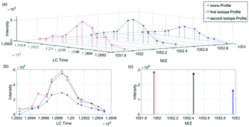Fig. 5 Peptide “EGGWDSVQDWMDVLSGGEK” isotope XICs in data 1 (Group 1). (a) Isotope XICs of peptite “EGGWDSVQDWMDVLSGGEK” in dataset 1, (b) isotope peak profile, (c) isotope distribution pattern.

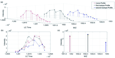Fig. 6 Peptide “EGGWDSVQDWMDVLSGGEK” isotope XICs in data 2 (Group 1). (a) Isotope XICs of peptite “EGGWDSVQDWMDVLSGGEK” in dataset 2, (b) isotope peak profile, (c) isotope distribution pattern.

DKL (P‖Q) described the information loss when the probability distribution Q was used to fit the distribution P, where P denoted the real distribution and Q denoted the fitting distribution of P. The closer the value of DKL (P‖Q) was to zero, the more consistent the two distributions were, that was, the more probably the two interval signal were generated by the same peptide. This paper took the value of natural logarithm for the obtained KL divergence values in order to distribute them in the whole coordinate axis.

Here, peak shape similarity feature was also calculated between the two peaks. It was described by calculating the linear regression determinant R² of the two peak sequences. As shown in Fig. 5 and 6, mono intervals of one peptide in data 1 and 2 could be considered as two series. The total sum of the squares SS_tot, regression sum of the squares SS_reg, error sum of the squares SS_res, and R² value were calculated as follows:

SS_tot = SS_res + SS_reg (2)

R² = SS_reg/SS_tot (3)

The R² value was between 0 and 1. If the two peaks were similar, the value should be close to 1. While not, it was close to 0.

Fig. 7 showed the histogram of the time difference, peak shape similarity and KL divergence of isotope distribution pattern between dataset 1 and 2 in Group 1. From the figure, the time difference feature was still a very important feature to distinguish the peak pair because the variance of the corresponding peak difference was much smaller than that of the non-corresponding one. However, the histogram of the non-corresponding peak time difference (d) still had an overlap (a) from −200 s to 100 s with a high intensity, which meant false positive judgement.

Fig. 7 Histogram of time difference, peak similarity and KL divergence. (a) Histogram of corresponding time difference. (b) Histogram of corresponding peak similarity. (c) Histogram of corresponding KL divergence. (d) Histogram of non-corresponding time difference. (e) Histogram of non-corresponding peak similarity. (f) Histogram of non-corresponding KL divergence.

Fig. 7 showed the histogram of peak shape similarity in (b) and (e). The overlap from 0.6 to 1 between corresponding and non-corresponding features in (b) and (e) was too obvious to be ignored, which could cause high false positive. Compared with the peak shape similarity, as shown in Fig. 7(c) was the histogram of ln(KL divergence value) of correlated peaks, and (f) was the histogram of ln(KL-divergence-value) of non-correlated peaks. By comparing these two graphs, the histogram of non-corresponding was distributed between −10 and 0 with high intensity from −5 to 0 in (f), while the corresponding ones were concentrated from −10 to −5 with just a few larger than −5 in (c). We could easily see that the discrimination got from the (c) and (f) was much better than that from (b) and (e), which meant that the isotope distribution pattern feature should have a stronger distinction characteristic with low false positive than peak shape feature.

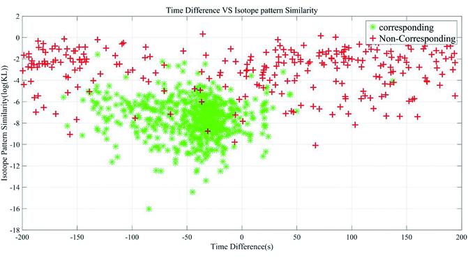
We selected time and isotope feature for both corresponding and non-corresponding peak pair and plotted the Fig. 8 based on the Group 1. This figure told us that it was necessary to find a classification curve that divided the area into two parts labelled as corresponding and non-corresponding. We tried the SVM classification model to verify the peak pair in a two-dimensional way to reduce the false positive rate. SVMs were supervised learning models with associated learning algorithms that analyze data used for classification and regression analysis. The training dataset we selected here were the peak pairs with labels in two categories of corresponding and non-corresponding. Thus, SVM could build a model with training data that assigned a new point to one category or the other. This was a non-linear classification problem (Fig. 8), and thus we tested four kernel functions in our algorithm: quadratic kernel, polynomial kernel, Gaussian radial basis function kernel, multilayer perceptron kernel. The results would be shown in the next section.

Fig. 8 Time and isotope pattern similarity of each peak pair.

2.2.4 Model testing & full-scale alignment and matching. Because the peptide peak pairs in the total training candidate peptide set were all with ground truth, we applied a 10-fold cross validation based on them to estimate the performance of the model: 90% was used as the training set and 10% was the validation set. This was repeated 10 times until all the peak pairs were validated once and then generated the average accuracy for the SVM classification model.

The difference set (zone 1 and zone 2 in Fig. 3) contained the peptides that were identified only once in only one dataset. After interval detection in the other datasets, several peak pairs with one real peak was generated. All of these peak pairs were put into the SVM classification model and verified as either corresponding or non-corresponding. The final result aligned and matched the peptide peaks in the union part as many as possible. The coverage rate was calculated by the number of matched over total number of peptides need to be matched, which was given in the next section.

3 Results and discussion

3.1 Model testing results

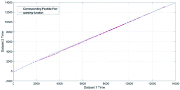
There were four parts in this section depending on the method we used, which were OpenMS, Warping function and the SVM model in this paper.

3.1.1 The result of OpenMS. We checked the performance of OpenMS in dataset 1 and 2 in Group 1. First We created two .edta files²⁷ according to the required data format with five columns: RT, m/z, intensity, charge, and mymeda. In the first file of Q1, we listed the intervals that contained the retention time points reported by tandem MS for every peptide in the testing set. In the second file of Q2, all candidate intervals for all testing peptides were listed. We subsequently converted the .edta files to .featureXML files using the function FileConverter in OpenMS. We then applied MapAligner to align the two featureXML files. Finally, we used FeatureLinker in OpenMS to find the corresponding features. In this step, the parameter max pair distance had two fields that require user input values: RT and MZ. We set RT to two possible values 500 and 700; MZ was set as 0.01. We tried different settings to ensure the best result. The processing procedure in OpenMS was shown in Fig. 9.

Fig. 9 Flowchart of OpenMS.

At last, we checked how many peptides with linked peak pair generated from OpenMS could be find in the intersection peptide list. It can achieve 81.67% accuracy in dataset Group 1 under these settings, which makes little difference to Warping functions.

3.1.2 The result of warping function. We used a polynomial fitting curve as the warping function to get the accuracy result based on the total training candidate peptide set. The warping curve based on dataset 1 and 2 in Group 1 was shown in Fig. 10.

Fig. 10 Warping Function.

The LC peak that was the closest to the mapped time point was considered to correspond to the real peak, and checked with the ground truth. The results of Group 1 were shown in Table 1.

Table 1 The result of Warping function of datasets in Group 1

Index	1	2	3	4	5	6	7	8	9	10
Accuracy (%)	0.8333	0.8333	0.8167	0.7833	0.8333	0.7833	0.8333	0.8500	0.7500	0.8333

---

The average accuracy was 81.50%, and the standard deviation was 0.030. The performance was almost similar to the OpenMS. If the elution time was shorter, then the real peak of a peptide would have much closer neighbor peaks. The warping function-based methods were less effective in aligning corresponding peaks.

Then we applied warping function in each two datasets in Group 2 and 3, which were calculated with 10-fold validation with the mean and standard deviation. The results were shown in Tables 2 and 3.

Table 2 The result of Warping function of datasets in Group 2

Index	Data 1 and data 2 in Group 2	Data 1 and data 3 in Group 2	Data 2 and data 3 in Group 2
Mean of accuracy (%)	0.8480	0.8171	0.8272
Standard deviation of accuracy	0.0251	0.0368	0.0236

---

Table 3 The result of Warping function of datasets in Group 3

Index	Data 1 and data 2 in Group 3	Data 1 and data 3 in Group 3	Data 2 and data 3 in Group 3
Mean of Accuracy (%)	0.8393	0.7867	0.8444
Standard deviation of accuracy	0.0209	0.0208	0.0155

---

Here we could see that the results of Warping function were stable around 82% for each datasets pair in Group 1, 2 and 3.

3.1.3 The result of SVM classification model. First, we tested four kernel functions in the SVM model (Fig. 11) based on Group 1.

Fig. 11 SVM classification model of four different kernels. (a) Quadratic, (b) Gaussian radial basis function, (c) polynomial, (d) multilayer perceptron kernel.

As the Fig. 11 showed, Gaussian kernel performed a little better and the accuracy result of Group 1 was based on the Gaussian kernel in Table 4.

Table 4 Accuracy result of SVM model in datasets Group 1

Index	1	2	3	4	5	6	7	8	9	10
Accuracy (%)	0.9681	0.9681	0.9656	0.9740	0.9681	0.9664	0.9723	0.9681	0.9673	0.9690

---

The average accuracy was 96.87%, and the standard deviation was 0.003. Fig. 12 plotted the receiver operating characteristic curves of the SVM classification model. The true positive rate could reach almost 97% with a false positive rate of 8%.

Fig. 12 ROC of SVM classification model.

We also applied SVM with Gaussian kernel in each datasets pair in Group 2 and 3. The results with mean and standard deviation were shown in Tables 5 and 6.

Table 5 Accuracy result of SVM model in datasets Group 2

Index	Data 1 and data 2 in Group 2	Data 1 and data 3 in Group 2	Data 2 and data 3 in Group 2
Mean of accuracy (%)	0.9057	0.9103	0.9485
Standard deviation of accuracy	0.0185	0.0166	0.0080

---

Table 6 Accuracy result of SVM model in datasets Group 3

Index	Data 1 and data 2 in Group 3	Data 1 and data 3 in Group 3	Data 2 and data 3 in Group 3
Mean of accuracy (%)	0.9733	0.9612	0.9693
Standard deviation of accuracy	0.0044	0.0077	0.0050

---

Here the results showed that the average accuracy of SVM were higher than Warping function. However, the SVM results of Group 1 and 3 were similar and a little better than Group 2. This might be cause by the experiment, because datasets of Group 1 and 3 were all from Velos instrument, while the Group 2 was generated by traditional Obitrap.

3.1.4 Hypothesis testing of SVM and warping method. We next examined if there was a significant improvement between the two methods via the Wilcoxon rank-sum test.

Method 1 was only based on the Warping Function (OpenMS obtained a similar result);

Method 2 was the SVM classification model.

The results of these two methods, which were all based on the same training and testing datasets in Group 1, were listed in Tables 1 and 4. We assumed no significant difference between the two methods. The hypotheses were as follows: H₀, there was no significant difference between the two methods;

H₁, there was a difference between the two methods.

The Wilcoxon rank sum tested at a significance level of 0.05 had a P-value of 0.001. The H value was 1, which rejected H₀ at a significance level of 5%. Thus, the data showed that method 2 performed much better than method 1. The SVM classification model used not only a time feature but also an isotope distribution pattern similarity to improve outcomes by almost 15%.

3.2 The coverage rate of the union dataset

First we checked the coverage rate of Group 1. The MS/MS information in Fig. 3 showed 4247 peptides in data 1 and data 2; 1944 peptides in zone 1; and 1603 peptides in zone 3. The total difference set contained 3547 peptides. After applying our SVM classification model, there were 3226 real peaks from 3547 peptides that matched the corresponding peak. The coverage rate reached 91.0%.

We also applied the model to match the difference set in Group 2 and 3. In Group 2, the data 1 and data 2 had the difference set of 11238 peptides, in which the coverage rate reached 75.67%. The data 1 and data 3 had the difference set of 9802 peptides with the coverage rate of 82.42%. The difference set of data 2 and data 3 contained 8130 peptides with coverage rate of 74.07%. In Group 3, the difference set of data 1 and data 2 contained 7912 peptides. The coverage rate reached 84.89%. The data 1 and data 3 had the difference set of 8354 peptides, in which the coverage rate was 76.66%. The difference set of data 2 and data 3 contained 8107 peptides with coverage rate of 88.50%. The coverage rate result was shown in Tables 7 and 8.

Table 7 The coverage rate of each datasets pair in Group 2

Index of the difference set	Data 1 and data 2 in Group 2 (11238 peptides)	Data 1 and data 3 in Group 2 (9802 peptides)	Data 2 and data 3 in Group 2 (8130 peptides)
Coverage rate (%)	0.7567	0.8242	0.7407

---

Table 8 The coverage rate of each datasets pair in Group 3

Index of the difference set	Data 1 and data 2 in Group 3 (7912 peptides)	Data 1 and data 3 in Group 3 (8354 peptides)	Data 2 and data 3 in Group 3 (8107 peptides)
Coverage rate (%)	0.8489	0.7666	0.8850

---

3.3 Discussion

These results showed that there were still some problems requiring further study.

First, the accuracy of interval detection needs to be improved. This paper used simple interval detection. The threshold was set to detect three times the standard deviation of the background noise in the high-intensity peak area. The interval should contain six consecutive points (values above the threshold were considered candidate LC peaks). Taken the dataset Group 1 as example, after interval detection, only 599 peptides were seen of the 700 that intersected from the MS/MS time point. The detection rate was 85%; thus, the interval detection algorithm needs to be improved.

Second, the results showed that the time discrimination was high, but it could not solve all problems-especially in the noisy XICs. The isotope distribution pattern similarity feature could improve this by almost 15%. However, there were still some non-corresponding peak pairs with a low time difference and a high isotope distribution pattern similarity. Thus, more features should be studied.

4 Conclusions

We used a SVM learning method based on the time difference and isotope distribution pattern similarity features in LC-MS replicated datasets, which was not based on the peak profile similarity as usual, but on the isotope distribution. This method was applied on three groups of datasets to align spectra and match the corresponding peak pairs. The accuracy could reach more than 90%, and most could be around 97%. The coverage rate were most around 80%, and some could reach nearly 91%.

Conflicts of interest

There are no conflicts to declare.

Acknowledgements

This work was supported the project of Shandong University Scientific Research Development Program (Grant No. J18KB071) in 2018, the National Innovation Training Program of Local Universities in 2017 (Grant No. 201713386028) and the Key Laboratory of Dongying. The data used in this study was provided by Michelle Zhang and RCMI Proteomics and Protein Biomarkers Cores at UTSA, who also gave great help for paper writing and revision. We also thanked LetPub (www.letpub.com) for its linguistic assistance during the preparation of this manuscript.

Notes and references

1. G. Palmisano, M. R. Larsen, N. H. Packerc and M. ThaysenAndersenc, RSC Adv., 2013, 3, 22706–22726.
2. R. Smith, D. Ventura and J. T. Prince, Briefings Bioinf., 2015, 16, 104–117.
3. S. B. Nielsen, J. U. Andersen, P. Hvelplund, T. J. D. Jorgensen, M. Sorensen and S. Tomita, Int. J. Mass Spectrom., 2002, 213, 225–235.
4. D. Bylund, R. Danielsson, G. Malmquist and K. E. Markides, J. Chromatogr. A, 2002, 961, 237–244.
5. A. P. Vilches, S. H. Norström and D. Bylund, J. Sep. Sci., 2017, 40, 1482–1492.
6. P. H. Eilers, Anal. Chem., 2004, 76, 404–411.
7. A. M. V. Nederkassel, C. J. Xu, P. Lancelin, M. Sarraf, D. A. Mackenzie, N. J. Walton, F. Bensaid, M. Lees, G. J. Martin and J. R. Desmurs, J. Chromatogr. A, 2006, 1120, 291–298.
8. J. T. Prince and E. M. Marcotte, Anal. Chem., 2006, 78, 6140–6152.
9. T. Górecki and M. Łuczak, Expert Systems with Applications, 2014, 42, 2305–2312.
10. R. Wehrens, T. G. Bloemberg and P. H. C. Eilers, Bioinformatics, 2015, 31, 3063–3065.
11. B. Walczak and W. Wu, Chemom. Intell. Lab. Syst., 2005, 77, 173–180.
12. M. Katajamaa and M. Orešič, BMC Bioinf., 2005, 6, 1–12.
13. N. Jaitly, M. E. Monroe, V. A. Petyuk, T. R. W. Clauss, J. N. Ad-kins and R. D. Smith, Anal. Chem., 2006, 78, 7397–7409.
14. E. Lange, R. Tautenhahn, S. Neumann and C. GröPl, BMC Bioinf., 2008, 9, 375.
15. B. Voss, M. Hanselmann, B. Y. Renard, M. S. Lindner, U. Kothe and M. Kirchner, Bioinformatics, 2011, 27, 987.
16. H. L. Röst, T. Sachsenberg, S. Aiche, C. Bielow, H. Weisser, F. Aicheler and S. A. Andreotti, et al., Nat. Methods, 2016, 13, 741–748.
17. J. Pfeuffer, T. Sachsenberg, O. Alka, M. Walzer, A. Fillbrunn, L. Nilse, O. Schilling, K. Reinert and O. Kohlbacher, J. Biotechnol., 2017, 261, 142–148.
18. M. Bellew, M. Coram, M. Fitzgibbon, M. Igra, T. Randolph and P. W. Wang, et al., Bioinformatics, 2006, 22, 1902–1909.
19. J. Eckels, P. Hussey, E. K. Nelson, T. Myers, A. Rauch, M. Bellew, B. Connolly, W. Law, J. K. Eng and J. Katz, Current Protocols in Bioinformatics, 2011, ch. 13, pp. 13.5.1–13.5.25.
20. M. Bantscheff, M. Schirle, G. Sweetman, J. Rick and B. Kuster, Anal. Bioanal. Chem., 2007, 389, 1017–1031.
21. C. Bielow, G. Mastrobuoni and S. Kempa, J. Proteome Res., 2015, 15, 777–787.
22. S. Tyanova, T. Temu and J. Cox, Nat. Protoc., 2016, 11, 2301.
23. J. Cox and M. Mann, Nat. Biotechnol., 2008, 26, 1367.
24. J. Cui, X. Ma, L. Chen and J. Zhang, BMC Bioinf., 2011, 12, 439.
25. M. G. Bari, X. Ma and J. Zhang, Bioinformatics, 2014, 30, 2464–2470.
26. X. Wei, W. Sun, X. Shi, I. Koo, B. Wang, J. Zhang, X. Yin, Y. Tang, B. Bogdanov and S. Kim, Anal. Chem., 2011, 83, 7668–7675.
27. M. Sturm, A. Bertsch, C. Gröpl, A. Hildebrandt, R. Hussong, E. Lange, N. Pfeifer, T. O. Schulz, A. Zerck and K. Reinert, BMC Bioinf., 2008, 9, 163.

---

Footnotes

† Electronic supplementary information (ESI) available: https://pan.baidu.com/s/1xCSMZK1Co2nQOV_rv0fDQA; all these files can be opened by Matlab. See DOI: 10.1039/c9ra03789f

‡ These authors contributed equally to this work.

---