DOI:
10.1039/C9RA00940J
(Paper)
RSC Adv., 2019,
9, 16187-16194
Interfacial tension measurements using a new axisymmetric drop/bubble shape technique†
Received
4th February 2019
, Accepted 7th May 2019
First published on 23rd May 2019
Abstract
This paper introduces a new mathematical model that is used to compute either the interfacial tension of quiescent axisymmetric pendant/sessile drops and pendant/captive bubbles. This model consists of the Young–Laplace equation, that describes interface shape, together with suitable boundary conditions that guarantee a prescribed volume of drops/bubbles and a fixed position in the capillary. In order to solve the problem numerically, the Young–Laplace equation is discretized by using numerical differentiation and the numerical solutions are obtained applying the well-know Newton method. The paper contains a validation of the new methodology presented for what theoretical bubble/drops are used. Finally, some numerical results are presented for both drops and bubbles of water as well as several surfactant solutions to demonstrate the applicability, versatility and reproducibility of the proposed methodology.
1 Introduction
Accurate calculation of surface tension has revealed essential in many applications: pulmonary surfactants at the alveolar liquid–air interface,1,2 generation of liquid foams,3 etc. Indeed, recently there is a high motivation for understanding the physicochemical behaviour of foams, with applications in diverse fields as in food and cosmetic products, metal mining or for injection and treatment of varicose veins, just to name a few. The coalescence of the bubbles in the foam is prevented by the addition of particles or surfactants which lower the surface pressure and stabilize such foams. Drop shape techniques for the measurement of interfacial tension are powerful, versatile and flexible. A key issue is that the shape of the interface is determined by a combination of surface tension and gravity effects as the Young–Laplace equation of capillarity establishes.4,5 Indeed, there are five parameters controlling the shape: gravity, density, holder diameter, drop/bubble volume and surface tension, the latter one being the only unknown parameter to be determined by comparison between experimental and theoretical profiles. The higher the surface tension is, the more spherical the interface becomes; on the contrary, gravity tends both to elongate a pendant drop/bubble or to flatten a sessile drop. One of the constraints of this method is the fact that when the drop shape is close to spherical, the shape variation with respect to change in the surface tension is small and, in some cases, close to the length of a pixel. Therefore it is important to work in an intermediate range of drop/bubble volume for which the deformation by gravity is large enough to make the interface more sensitive to surface tension variations.
Determining interfacial tension from a liquid/fluid interface shape has been a challenging scientific issue in recent years due to the advance of image analysis and numerical methods along with the increasing of the computational capacity of computers. In 1883 Bashforth and Adams6 pioneered the mathematical analysis of axisymmetric drops tabulating the solutions of the differential equations describing the drop profile in terms of the surface tension and the radius of curvature at the apex. Since then several methods have been developed to compute the value of interfacial tension: γ-PD-FEM, see ref. 7, theoretical image fitting analysis (TIFA), see ref. 8, Axisymmetric Drop Shape Analysis (ADSA), see ref. 9–14 and the references therein, the latter one being the standard and widely used worldwide. ADSA methods are based on minimizing the distance between the experimental axisymmetric bubbles, or drops, and a theoretical profile of the interface obtained from the Young–Laplace equation written as a system of three first-order ordinary differential equations in terms of the arc length of the profile. Axisymmetric Drop Shape Analysis Profile (ADSA-P) is considered here a standard code in order to validate the methodology proposed in this work.
The new contribution of our work is to introduce a new methodology to numerically solve the Young–Laplace equation using the Newton method to its discretized version obtained by means of numerical differentiation; it allows to fix the volume of the bubble (or drop) as well as its position on the capillary. As a result, two MATLAB codes have been implemented: TEN2PRO which calculates the bubble (or drop) numerical profile from the surface tension, and, reciprocally, PRO2TEN that calculates the surface tension from an experimental axisymmetric form of a bubble (or drop). Theoretical interfaces with known interfacial tension have been generated to numerically validate the codes and, finally, this methodology has been applied to experimental profiles and the results compared with those provided by ADSA-P.
2 Experimental procedure
2.1 Materials
Different solutions with different concentrations of 1-decanol (99%, Sigma Aldrich) in MilliQ water were prepared after cleaning the flasks with soap (Micro-90, Sigma Aldrich) and subsequent rinsing with tap water, distilled water, propanol (99%, Sigma Aldrich), distilled water and MilliQ water. This protocol is necessary to ensure that the interfacial activity is due exclusively to the addition of the decanol. Depending on the volume of initial decanol that we mixed with MilliQ water, we used a 50 μl plastic Pasteur pipette (for solutions above 10−7 mol cm−3) or a 10 μl microsyringe (for solutions below 10−8 mol cm−3), where we rinsed the latter with chloroform (HPLC grade, Sigma Aldrich) before and after each deposition. Once we deposited the required amount of decanol into a 500 ml volumetric flask, we completed up to 500 ml of MilliQ water. After closing the flask with a stopper we shaked vigorously and ultrasonicated for 10 minutes. After this, the solution was kept at room temperature overnight. Because the decanol has a very low solubility in water (3.7 g l−1), it was expected that in MilliQ water (0.0054 μS cm−1) it would present a significantly lower solubility. In fact, at higher concentrations a significant fraction of the decanol remained segregated from the MilliQ water even after mixing and ultrasonication. Thus, we prepared each concentration tested from a different mixture of decanol and water, instead of successive dilutions of a master batch, to try to avoid effects from this segregation process.
2.2 Pendant bubble device
The pendant bubble tensiometer allows to change and control the volume of an air bubble attached to a capillary immersed in a liquid phase. The device consists, see Fig. S1 in the ESI,† of a Teflon capillary with a diameter of 2.95 mm immersed in a quartz cuvette (Sigma Aldrich) filled with the water-decanol solution. The capillary is attached to a Hamilton microinjector which we used to inject a given air volume and the cuvette and capillary were previously cleaned with the same protocol as described in the previous section. The cuvette was illuminated with a diffuse light source and live video was obtained with a CCD camera. The images were processed and archived in Dinaten, software developed in the Laboratory of Surfaces and Interfaces, in the University of Granada.
The software takes advantage of the axisymmetric nature of the pendant bubbles. Real time bubble images are processed via ADSA-P giving the pendant bubble volume and surface tension as results. Each experiment begun by filling the cuvette with the desired solution of decanol in MilliQ water, immersing the capillary and injecting a test bubble to locate the ends of the capillary. Then, starting from the capillary without a bubble, an initial bubble of 10 μl was injected and just after that the volume was maintained constant over time. During this evolution the shape of the bubble was changing as the surface tension was decreasing due to the interfacial adsorption of decanol. We took images every 0.2–0.3 s the first 15 seconds and then every second up to 1000 s to ensure proper volume control. The ADSA-P technique fails for spherical profiles which typically occur when the bubble is small and the gravity (buoyancy for bubbles) barely deforms their shapes. For big bubbles the interfacial tension decrease may cause the falling or creaming of the bubble, respectively. Thus, we needed to work in an intermediate range in which the deformation by gravity was large enough to apply ADSA-P but the deformation was low enough so the bubble remained attached to the capillary. For low concentrations of decanol it was possible to form a 40 μl pendant bubble, but as the tension decreased with higher concentrations of decanol, the bubble detached from the capillary and we had to decrease the volume of the pendant bubble down to 20 μl for the highest decanol concentration. All measurements were made at a temperature of 18 °C and a humidity of 70%.
2.3 Pendant drop device
Surface tension of a gemini surfactant, 1,4-butanediaminium,N,N,N,N-tetramethyl-N,N-ditetradecyl bromide (14-4-14), has been obtained by pendant drop method. Pendant drops of different volumes with different surfactant concentrations were suspended from a needle in a quartz cell kept at constant temperature (25 °C). Gemini concentrations were 4 × 10⁻⁸ mol cm−3 and 1 × 10⁻⁷ mol cm−3. The surface tension was calculated from the shadow image of a pendant drop using drop shape analysis.
3 Mathematical model
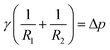
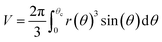
There are several different experimental techniques for measuring interfacial properties of a solution, being widely used the ones that are based on the analysis of the profile of pendant/sessile drops or pendant/captive bubbles, see Fig. 1(a). Assuming that all the involved fluids are quiescent, the interface location is determined by a static balance between interfacial surface tension and gravitational force as the Young–Laplace equation states. This expression, that relates the pressure difference at the interface to the interfacial tension and the curvature, can be written as follows (see ref. 5)| |
 | (1) |
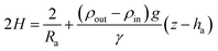
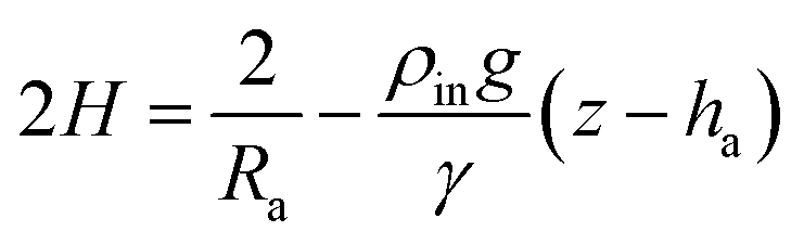
γ being the interfacial tension, R1 and R2 the principal radii of curvature and Δp the pressure difference at the interface. Taking into account only hydrostatic contributions to the pressure and axisymmetric interfaces, see Fig. 1(b), we obtain| | |
Δp = Δp0 + (ρout − ρin)g(z − ha)
| (2) |
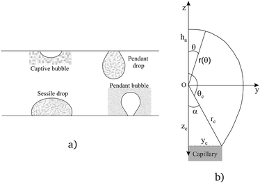 |
| | Fig. 1 Drop/bubble configurations (a), coordinate system and pendant bubble profile (b). | |
| | |
γ(2H) = Δp0 + (ρout − ρin)g(z − ha)
| (3) |
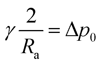
Taking into account that for axisymmetric interfaces the principal radii of curvature at the apex coincide, at z = ha eqn (3) gives
| |
 | (4) |
Ra being the curvature radius at the apex. Since
γ is a positive constant, from
eqn (3) and
(4) we obtain
| |
 | (5) |
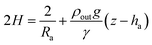
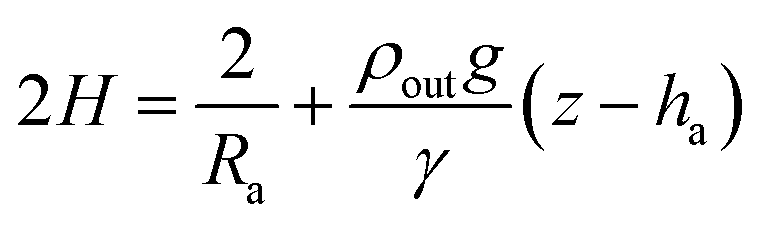
Notice that for a pendant bubble on a inverted needle, see Fig. 1(a), ρout ≫ ρin, z − ha ≤ 0 and eqn (5) can be approximated by
| |
 | (6) |
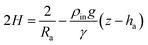
Remark 1. Furthermore, for a sessile drop ρin ≫ ρout and z − ha ≤ 0, then eqn (5) leads to
| |
 | (7) |
On the other hand, for a captive bubble ρout ≫ ρin and z − ha ≥ 0, and from (5) we get (6). Finally, for a pendant drop ρin ≫ ρout, z − ha ≥ 0 and (5) gives (7).
Summarizing, eqn (6) characterizes the profile of a pendant/captive bubble while eqn (7) describes the shape of a sessile/pendant drop. In what follows in this section and in the following one, we work with a pendant bubble, see Fig. 1(b), but we notice that the same reasoning we employ here is also valid for both sessile and pendant drops and for captive bubbles.
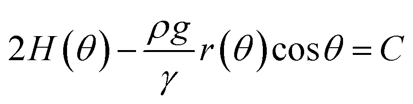
Now, for solving the Young–Laplace eqn (6) numerically, we need to obtain a discrete version of it. In order to do that, we use a spherical parametrization of the pendant bubble depicted in Fig. 1(b), that is introduced in Section 2 of the ESI.† For a pendant bubble on a inverted needle, the Young–Laplace eqn (6) must be verified at the surface. Straightforwardly, taking into account the information given in the ESI,† (6) yields
| |
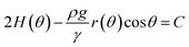 | (8) |
where, for reader's sake, we have omitted the subscript in the symbol of the density. We notice that, in the previous equation, both the constant
C and the function
r(·) are unknown. Therefore, in this problem, we look for the constant
C and the distances between the origin and the bubble points, that are given by function
r(·), as it is shown in
Fig. 1(b). Since
(8) is a second-order ordinary differential equation, two boundary conditions must be given in order to be solved. Moreover, the unknown constant
C requires an extra boundary condition. We choose them as follows:
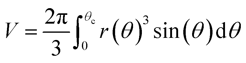
Notice that condition (9) states that the profile at the apex is perpendicular to the z-axis; furthermore, condition (10) stands for the capillary radius. We remark here that one of the novelties of this work is given by boundary condition (10), since it guarantees a fixed capillary position in contrast with ADSA methods.5 The third condition is established in terms of the bubble volume which is a constraint of the problem. So, we have
| |
 | (11) |
Details of calculations indicating how to obtain the numerical solutions are reported in Section 3 of the ESI.†
4 Results and discussion
4.1 Direct problem
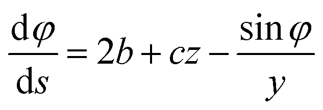
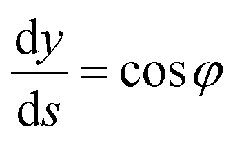
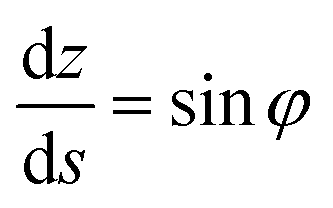
The methodology presented above has been implemented in the MATLAB computer code TEN2PRO – TENsion TO PROfile – to obtain numerical profiles of drops and bubbles. For validation purposes, we have considered theoretical drops and bubbles of several volumes, generated by solving the following system of ordinary differential equations, introduced by Bashforth and Adams, see ref. 5, 9 and 11 and the references therein:| |
 | (12) |
| |
 | (13) |
| |
 | (14) |
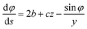
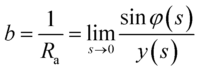
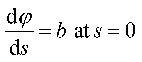
φ being the angle between the tangent line at the interface with the horizontal and s the arc length measured from the apex of the drop (or bubble). The positive constant b is the curvature at the apex. Notice that the capillary constant, c = ρg/γ, has positive values for sessile drops and negative values for pendant bubbles, see ref. 11. The initial conditions are
To avoid the indetermination in (12) at the apex (s = 0), we use
and
(12) yields
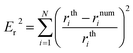
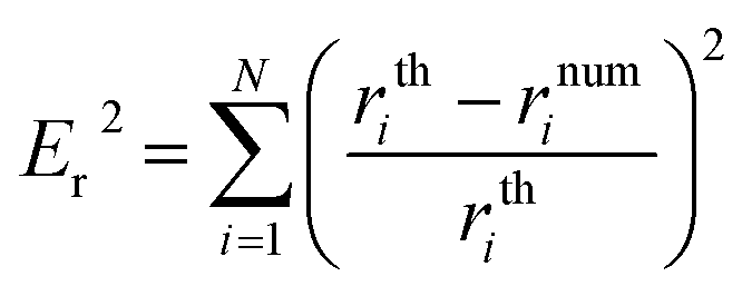
The solution of the previous system is obtained in MATLAB using a well-known Runge–Kutta method with an error tolerance of 10−10. Its solution is taken as the theoretical profile in order to validate the code TEN2PRO. Hereafter in this section, density and gravitational constant are taken as follows: ρ = 998.7 kg m−3 and g = 9.8 m s−2. Using the data γ = 0.06121 N m−1 and Ra = 0.001 m, a theoretical pendant bubble of 5 μl is obtained numerically solving (12)–(14). Its volume, the coordinates of the contact point, ρ, g and γ are the input parameters of the numerical code TEN2PRO with its output parameters being the profile of the bubble and the curvature radius at the apex. Both theoretical and numerical profiles are shown in Fig. 2. Analogously, theoretical bubbles of 20 μl and 30 μl are obtained for the data γ = 0.03669 N m−1, Ra = 0.001396 m and γ = 0.072767 N m−1, Ra = 0.00171 m, respectively. Theirs respective volumes, coordinates of the contact point and tension are the input parameters of the numerical code TEN2PRO. A spherical profile is chosen as the initial profile in the Newton algorithm. The profiles of the numerical bubbles are also shown in Fig. 2. No difference is appreciated and both results coincide. In Table 1 the relative error on the radial coordinate between numerical and theoretical bubbles—denoted by num and th superscripts, respectively—is presented in terms of the size of the partition N (i.e. the number of nodes in which the numerical solution is calculated):
| |
 | (15) |
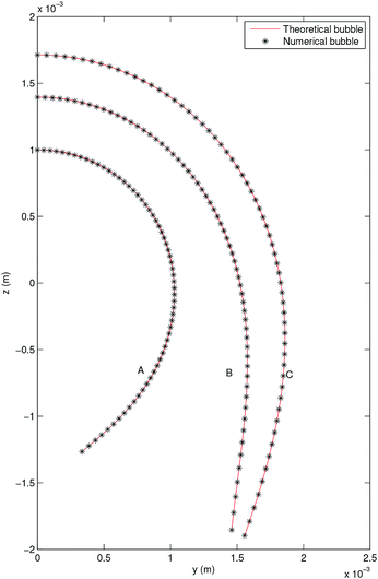 |
| | Fig. 2 Pendant bubble profiles of theoretical (—) and numerical (*) bubbles. (A) V = 5 μl, (B) V = 20 μl, (C) V = 30 μl. | |
Table 1 Relative error for pendant bubbles
| Direct problem |
| N |
Er (V = 5 μl) |
Er (V = 20 μl) |
Er (V = 30 μl) |
| 60 |
3.2 × 10⁻³ |
3.6 × 10⁻³ |
9.2 × 10⁻⁴ |
| 120 |
1.8 × 10⁻³ |
2.8 × 10⁻³ |
2.9 × 10⁻⁴ |
| 240 |
1.6 × 10⁻³ |
3.2 × 10⁻³ |
5.8 × 10⁻⁵ |
| Inverse problem |
| N |
er (B1) |
er (B2) |
er (B3) |
| 60 |
4.80 × 10⁻³ |
1.84 × 10⁻³ |
3.70 × 10⁻³ |
| 120 |
1.22 × 10⁻³ |
4.49 × 10⁻⁴ |
9.26 × 10⁻⁴ |
| 240 |
3.04 × 10⁻⁴ |
9.67 × 10⁻⁵ |
2.25 × 10⁻⁴ |
The same methodology can be applied to sessile drops as it can be seen in Section 4 of the ESI.†
4.2 Inverse problem
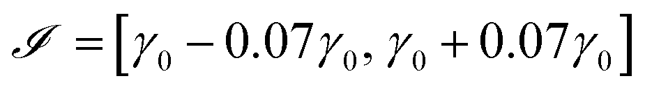
In this section, the methodology presented above is used to obtain the interfacial tension value from a given drop/bubble profile. It has been implemented in the MATLAB computer code PRO2TEN – PROfile TO TENsion – which proceeds as follows: after determining a searching interval for the tension, a simple bisection procedure in tensions is performed in order to find the numerical profile which fits the prescribed one. For code validation purposes, theoretical profiles of several volumes with known tension and curvature are generated solving system (12)–(14). In each case it is necessary to know the volume and the coordinates of the contact point. The searching interval is computed exploiting the fact that the mean curvature is linear with respect to z as the Young–Laplace equation states. Thus, an initial tension, γ0, is computed by linear least squares regression and the searching interval is taken as 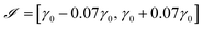 . On this interval, a bisection algorithm is used to find a root of the function β(γ) = r1(γ) − r1,exp, where r1,exp is the value of the radial coordinate of the experimental interface at the angle θa. For any choice of the tension γ, the Newton algorithm described in Section 3 in the ESI† is used to obtain a numerical profile taking the experimental state as the initial one. Using the data γ = 0.07291 N m−1, ρ = 1000 kg m−3 and Ra = 0.001 m, a theoretical pendant bubble of 4.86 μl—denoted hereafter by B1—is obtained. Its profile is the input parameter of the numerical code PRO2TEN, and its output parameter leads to the value of the interfacial tension. Both theoretical and numerical profiles are shown in Fig. 3. Analogously, theoretical bubbles of 37.19 μl—denoted by B2—and 717.23 μl—denoted by B3—are obtained for the data γ = 0.07291 N m−1, Ra = 0.001713 m and γ = 0.98064 N m−1, Ra = 0.005 m, respectively. The profiles of the numerical bubbles are also shown in Fig. 3.
 |
| | Fig. 3 Pendant bubble profiles of theoretical (—) and numerical (*) bubbles, where y and z axes represent distance measured in meters. (A) Bubble B1, (B) bubble B2, (C) bubble B3. | |
In Table 1 the relative error between numerical and theoretical interfacial tension—denoted by num and th superscripts, respectively—, er = |γnum − γth|/γth, is presented in terms of the size of the partition N.
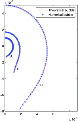
In order to simulate experimental interfaces obtained from digital images (like that described in ref. 14), artificial randomized errors of several amplitudes in the range of the pixel size are added to the radial coordinate using the MATLAB function rand as seen in Fig. 4. In order to find the searching interval for tensions, an image denoising procedure in terms of the biharmonic heat equation is used (see ref. 15), trying to reduce the noise part from the original surface but preserving its geometric features; in Fig. 4 the mean curvature versus z is shown for bubble B2 prior to and after using the denoising algorithm, in the latter the linear behaviour of the mean curvature is appreciable, which is used to compute an initial tension, γ0, and the searching interval. Performing ten runs of the code for each interface and amplitude, the mean interfacial tension, γm, is computed together with its relative error, er = |γm − γth|/γth, which is shown in Table 2 for N = 120.
 |
| | Fig. 4 Original and randomized profile (a) and zoom (b) in bubble B1. Mean curvature prior to (c) and after (d) performing the denoising algorithm in bubble B2. | |
Table 2 Relative error for pendant bubbles with randomized errors
| Error amplitude (m) |
er (B1) |
er (B2) |
er (B3) |
| 10−6 |
8 × 10⁻⁴ |
4 × 10⁻⁴ |
9 × 10⁻⁴ |
| 3 × 10⁻⁶ |
0.0272 |
2 × 10⁻⁴ |
10−3 |
| 6 × 10⁻⁶ |
0.0597 |
7 × 10⁻⁴ |
0.0179 |
| 9 × 10⁻⁶ |
0.0288 |
2 × 10⁻⁴ |
0.0349 |
4.3 Validation with experimental results
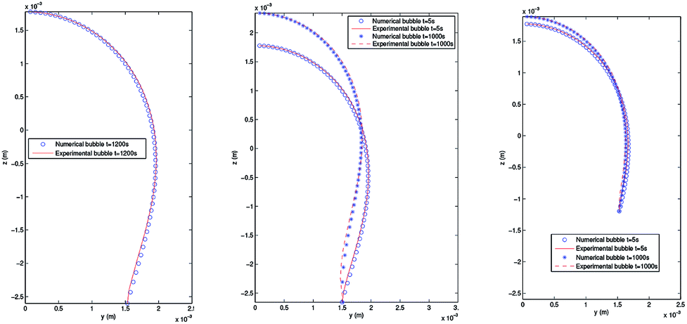
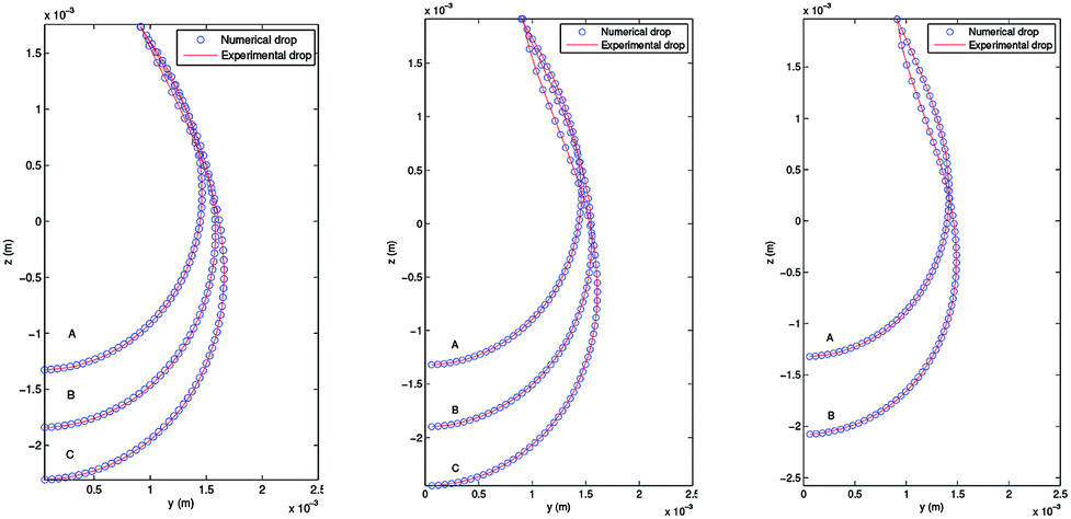
4.3.2 Pendant bubble into decanol aqueous solution. As stated above, this new methodology for the determination of interfacial surface tension has the advantage to keep the volume and the position of the bubble in the capillary constant. This possibility is of great importance in order to study processes of dynamic surface tension because it allows its implementation and automation in software protocols. In order to verify the validity of PRO2TEN in dynamic processes it has been applied to air bubbles into water and decanol aqueous solutions at several concentrations. Decanol adsorption kinetics by using pendant bubble tensiometer have been previously reported16 showing that surface tension equilibration needs 100–1000 s depending on the concentration. The time required to create an air bubble of 20–40 μl is about 0.1 s and afterwards the change in volume, as the surface tension relaxes during the adsorption of decanol onto the clean interface, is only a few percent over the time period of the experiment, allowing us to assume that the bubble volume keeps constant. Regarding decanol solutions, the process begins with a clean interface that is later occupied by the surfactant molecules until the equilibrium tension is reached. Fig. 6 shows the experimental and numerical pendant air bubbles for water and decanol aqueous solution for different times: an air bubble (V = 40 μl) into water at t = 1200 s, a bubble (V = 40 μl) into 4.7 × 10⁻⁸ mol cm−3 decanol aqueous solution at t = 5 s and t = 1000 s, and finally, a bubble (V = 20 μl) into 1.2 × 10⁻⁷ mol cm−3 decanol aqueous solution at t = 5 s and t = 1000 s. Notice that a good agreement is reached between the experimental and calculated profiles.
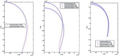 |
| | Fig. 6 Experimental and numerical pendant bubbles with several volumes at different times. Left: Air bubble (V = 40 μl) into water at t = 1200 s. Center: Air bubble (V = 40 μl) into 4.7 × 10⁻⁸ mol cm−3 decanol aqueous solution at t = 5 s and t = 1000 s. Right: Air bubble (V = 20 μl) into 1.2 × 10⁻⁷ mol cm−3 decanol aqueous solution at t = 5 s and t = 1000 s. | |
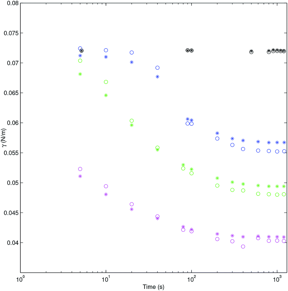
The interfacial tension versus time is shown in Fig. 7 for both codes ADSA and PRO2TEN. It shows representative dynamic surface tension profiles of decanol aqueous solutions at three different bulk concentrations and bubble volumes ranging from 20 to 40 μl. Additionally surface tension of bulk water at different bubble age are shown for comparative proposes. Closer inspection of Fig. 7 shows the good agreement between dynamic surface tension values obtained by application of ADSA and PRO2TEN. It is worth mentioning again the advantage of PRO2TEN methodology compared to ADSA by keeping constant the localization of the bubble in the capillary. This methodology will be very useful in order to automatize dynamic surface tension calculations by considering the continuous evolution of bubble shape with time, see Fig. S3 in Section 5 of the ESI,† and, consequently, the surfactant adsorption at a distorted bubble instead a spherical one.
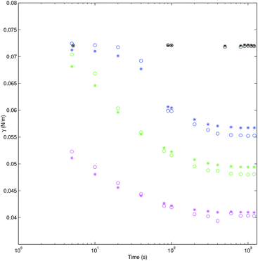 |
| | Fig. 7 Tension (N m−1) of decanol aqueous solution for ADSA (*) and PRO2TEN (○) at several concentrations versus time (s) in log scale: black 0 mol cm−3 and air bubble of 40 μl; blue 4.7 × 10⁻⁸ mol cm−3 and air bubble of 40 μl; green 8.3 × 10⁻⁸ mol cm−3 and air bubble of 35 μl; magenta 1.2 × 10⁻⁷ mol cm−3 and air bubble of 20 μl. | |
5 Conclusions
A new methodology in order to compute the profile of an axisymmetric bubble or drop from its surface tension and vice versa has been introduced yielding to accurate results both for theoretical and experimental profiles. It consists of numerically solving the Young–Laplace equation by applying the Newton method to its discretized version, obtained by means of numerical differentiation. The main advantage of this method is that it allows to set in advance the volume enclosed by the bubble/drop as well as its position on the capillary; this fact becomes very important in order to study processes of dynamic surface tension because it allows its implementation and automation in software protocols. Two computer codes have been developed using this methodology, TEN2PRO and PRO2TEN, and both have been tested against the standard code in this area, ADSA, providing a good agreement on the results.
Pendant bubble and pendant drops tensiometers have been employed to obtain experimental interface profiles enclosing different volumes and using two surfactants, decanol and gemini, with several concentrations.
Conflicts of interest
There are no conflicts to declare.
Acknowledgements
Authors thank to Dr J. A. Holgado-Terriza for the software Dinaten© used for surface tension measurements. Authors thank to Dr Xerardo Prieto and Mr Vicente Dominguez from the Universidad de Santiago de Compostela for the gemini surfactant measurements. This work has been supported by Ministerio de Economía y Competitividad under the Projects MTM2015-66640-P, CTQ2014-55208-P, CTQ2017-84354-P and PGC2018-096696-B-I00, Xunta de Galicia (GR 2007/085; IN607C 2016/03 and Centro singular de investigación de Galicia accreditation 2016-2019, ED431G/09) and the European Union (European Regional Development Fund-ERDF), is gratefully acknowledged.
References
- A. Jyoti, R. M. Prokop, J. Li, D. Vollhardt, D. Y. Kwok, R. Miller, H. Möhwald and A. W. Neumann, Colloids Surf., A, 1996, 116, 173–180 CrossRef CAS.
- S. M. I. Saad, Z. Policova, E. J. Acosta, M. L. Hair and A. W. Neumann, Langmuir, 2009, 25, 10907–10912 CrossRef CAS PubMed.
- W. Drenckhan and A. Saint-Jalmes, Adv. Colloid Interface Sci., 2015, 222, 228–259 CrossRef CAS PubMed.
- S. M. I. Saad and A. W. Neumann, Adv. Colloid Interface Sci., 2016, 238, 62–87 CrossRef CAS PubMed.
- M. Hoorfar and A. W. Neumann, Adv. Colloid Interface Sci., 2006, 121, 25–49 CrossRef CAS PubMed.
- F. Bashforth and J. C. Adams, An Attempt to Test the Theory of Capillary Action, Cambridge University Press, London, 1883 Search PubMed.
- N. M. Dingle, K. Tjiptowidjojo, O. A. Basaran and M. T. Harris, J. Colloid Interface Sci., 2005, 286, 647–660 CrossRef CAS PubMed.
- M. G. Cabezas, A. Bateni, J. M. Montanero and A. W. Neumann, Colloids Surf., A, 2005, 255, 193–200 CrossRef CAS.
- Y. Rotenberg, L. Boruvka and A. W. Neumann, J. Colloid Interface Sci., 1983, 93, 169–183 CrossRef CAS.
- P. Cheng, D. Li, L. Boruvka, Y. Rotenberg and A. W. Neumann, Colloids Surf., 1990, 43, 151–167 CrossRef CAS.
- O. I. Río and A. W. Neumann, J. Colloid Interface Sci., 1997, 196, 136–147 CrossRef PubMed.
- A. Kalantarian, R. David, J. Chen and A. W. Neumann, Langmuir, 2011, 27, 3485–3495 CrossRef CAS PubMed.
- S. M. I. Saad and A. W. Neumann, Adv. Colloid Interface Sci., 2014, 204, 1–14 CrossRef CAS.
- Y. Zuo, M. Ding, A. Bateni, M. Hoorfar and A. Neumann, Colloids Surf., A, 2004, 250, 233–246 CrossRef CAS.
- W. Zhu and T. Chan, SIAM J. Imag. Sci., 2012, 5, 1–32 CrossRef.
- S.-Y. Lin, T.-L. Lu and W.-B. Hwang, Langmuir, 1995, 11, 555–562 CrossRef CAS.
Footnote |
| † Electronic supplementary information (ESI) available. See DOI: 10.1039/c9ra00940j |
|
| This journal is © The Royal Society of Chemistry 2019 |
Click here to see how this site uses Cookies. View our privacy policy here. 
 Open Access Article
 This Open Access Article is licensed under a Creative Commons Attribution-Non Commercial 3.0 Unported Licence
 c,
L. García-Río
c,
L. García-Río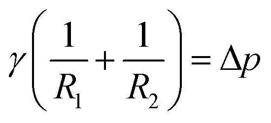


 . On this interval, a bisection algorithm is used to find a root of the function β(γ) = r1(γ) − r1,exp, where r1,exp is the value of the radial coordinate of the experimental interface at the angle θa. For any choice of the tension γ, the Newton algorithm described in Section 3 in the ESI† is used to obtain a numerical profile taking the experimental state as the initial one. Using the data γ = 0.07291 N m−1, ρ = 1000 kg m−3 and Ra = 0.001 m, a theoretical pendant bubble of 4.86 μl—denoted hereafter by B1—is obtained. Its profile is the input parameter of the numerical code PRO2TEN, and its output parameter leads to the value of the interfacial tension. Both theoretical and numerical profiles are shown in Fig. 3. Analogously, theoretical bubbles of 37.19 μl—denoted by B2—and 717.23 μl—denoted by B3—are obtained for the data γ = 0.07291 N m−1, Ra = 0.001713 m and γ = 0.98064 N m−1, Ra = 0.005 m, respectively. The profiles of the numerical bubbles are also shown in Fig. 3.


![[thin space (1/6-em)]](https://www.rsc.org/images/entities/char_2009.gif)