
 Open Access Article
 This Open Access Article is licensed under a Creative Commons Attribution-Non Commercial 3.0 Unported Licence
Effect of external electric field on nanobubbles at the surface of hydrophobic particles during air flotation
Leichao Wu,
Yong Han *,
Qianrui Zhang and
Shuai Zhao
*,
Qianrui Zhang and
Shuai Zhao
Measurement Technology and Instrumentation Key Laboratory of Hebei Province, School of Electrical Engineering, Yanshan University, Qinhuangdao 066004, P. R. China. E-mail: hanyong@ysu.edu.cn
First published on 14th January 2019
Abstract
In this paper, the effect of external electric field on nanobubbles adsorbed on the surface of hydrophobic particles during air flotation was studied by molecular dynamics simulations. The gas density distribution, diffusion coefficient, viscosity, and the change of the angle and number distribution of hydrogen bonds in the system with different amounts of gas molecules were calculated and compared with the results without an external electric field. The results show that the external electric field can make the size of the bubbles smaller. The diffusion coefficient of the gas increases and the viscosity of the system decreases when the external electric field is applied, which contribute to the reduction of the size of the nanobubbles. At the same time, comparing with the results under no external electric field, the angle of hydrogen bonding under the external electric field will increase, and the proportion of water molecules containing more hydrogen bonds will reduce, which further explains the reason why the external electric field reduces the viscosity. The conclusions of this paper demonstrate at the micro level that the external electric field can enhance the efficiency of air-floating technology for the separation of hydrophobic particles, which may provide meaningful theoretical guidance for the application and optimization of electric field-enhanced air-floating technology in practice.
1. Introduction
Since Parker1 first observed the presence of nanobubbles using atomic force microscopy (AFM) 20 years ago, nanobubbles formed on the liquid–solid surface quickly attracted widespread attention.2–5 Nanobubbles have many unique properties, such as long lifetimes, slow dissolution rates and large specific surface areas etc.6–8 Many hypotheses have been proposed to explain these properties, for instance, line tension theory,9 dynamic equilibrium model theory,10 impurity layer theory,11 three-phase contact line theory.12 But there is no theory that can perfectly explain the problems of nanobubbles.Although the mystery of nanobubbles at the theoretical level still needs further research, the separation of hydrophobic solid particles by bubbles in mineral flotation has been widely applied. Tao13,14 found the use of hydrodynamic cavitation to form bubbles on coal surfaces in recent flotation research, which can significantly improve the efficiency of flotation recovery. Hampton15 pointed out that the effect of high-concentration salt environment on the bubbles formed by mineral flotation is negligible, but the surface characteristics of solid particles have undergone tremendous changes. Fan16 found that nanobubbles with smaller diameters can significantly reduce the rate of bubble rise and create more favorable conditions for the flotation of hydrophobic particles. It can be seen that the size of the nanobubble and the environment of the solution will have an impact on the flotation effect. Therefore, how to improve the separation efficiency of hydrophobic particles by bubbles in mineral flotation has become the focus of attention.
In recent years, with the development of physical water treatment technology17–19, the combination of an external electric or magnetic field and flotation technology has provided a new field. Thiebaut20 found that the electromagnetic field enhances the effect of the collector on the flotation of fluorite ore. Birinci21 studied the flotation of a binary mixture of quartz and magnetite under the action of a magnetic field. The results shown that the magnetic field can significantly improve the separation efficiency. Murugananthan22 studied the method of separating suspended solids, sulfides and other contaminants by electric field flotation technology. The study found that the method is at least 20% more efficient than the traditional method. Although experiments have shown that an external electric or magnetic field can improve the efficiency of flotation in mineral separation, its mechanism of action remains unclear.
Therefore, the effects of external electric field on nanobubbles adsorbed on the surface of hydrophobic particles were studied by molecular dynamics simulation. The mechanism of the external electric field on the efficiency of air-floating separation was explored from the micro level, which may provide a useful guidance for combination of electric field and air-floating technology.
2. Model and simulation details
In order to mimic the adsorption of nanobubbles on hydrophobic particles, according to existing research methods,23,24 a box of 5.82 nm × 5.88 nm × 5.74 nm which is first filled with 6010 water molecules was built. The SPCE25 model was used for water molecules, because it has been proved to have good performance in the study of nanobubbles at hydrophobic solid–water interface.26 Then, the graphene model27,28 was used to replace the surface of hydrophobic particles on the bottom of the box, this method have been widely used in the molecular dynamic simulation.23,24 Finally, the 60, 120 and 180 CO2 molecules were randomly placed to form a gas–liquid–solid three-phase system with different amounts of gas molecules. The EPM2 carbon dioxide potential energy model29 was adopted as gas molecule, because it provides good prediction of the different situation30,31 (in a wide range of temperatures and pressures). Fig. 1 is a schematic diagram of the initial model.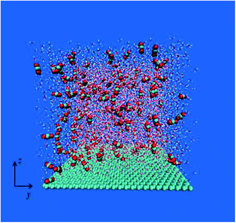 | ||
| Fig. 1 Schematic diagram of the initial configuration of the simulation. For clarity, the red ball represents the O atom, the cyan ball represents the C atom, and the water molecule is given in the form of a line. | ||
The OPLS-AA force field32 was adopted in all simulations. The force field parameters of graphene, water and gas molecule used in this study are summarized in Table 1.
| Atom | Molecule | σ (nm) | ε (kJ mol−1) | charge (e) |
|---|---|---|---|---|
| O | Water | 0.3166 | 0.6502 | −0.8476 |
| H | Water | 0 | 0 | 0.4238 |
| C | Graphite | 0.3400 | 0.3700 | 0 |
| CO | Carbon dioxide | 0.2757 | 0.2338 | 0.6512 |
| OC | Carbon dioxide | 0.3033 | 0.6690 | −0.3256 |
All the simulations were performed with the GROMACS package (version 5.1.2).33 The time step for leapfrog method was 1 fs, the system temperature was controlled at 300 K, using velocity rescaling. Particle mesh Ewald (PME)34 was used to calculate the long-range electrostatic interaction. The cut-off distance for Lennard-Jones interactions was 1.2 nm. To avoid the unpredictable effect of high electric field intensity on water molecules and graphene.35,36 The electric field intensity of 0.1 V nm−1 was applied along a given direction (corresponding to the y-axis in Fig. 1, parallel to the graphene membrane). All the simulations including 500 ps for equilibrium period and 10 ns for sampling stage was used to calculate the properties.
3. Results and discussion
3.1 Density distribution of gas
The adsorption of bubbles on the hydrophobic particles produces different shapes.37–40 Different shapes affect the size of the contact area between bubbles and the hydrophobic particles and the contact time. Under the action of the external electric field, the shape of the bubble will also change.41 Therefore, it is necessary to explore the shape change of the bubble under the external electric field. In this paper, the morphology of bubbles on the hydrophobic interface in a solution system with different CO2 dissolved gases under the external electric field were studied. The simulation results are shown in Fig. 2.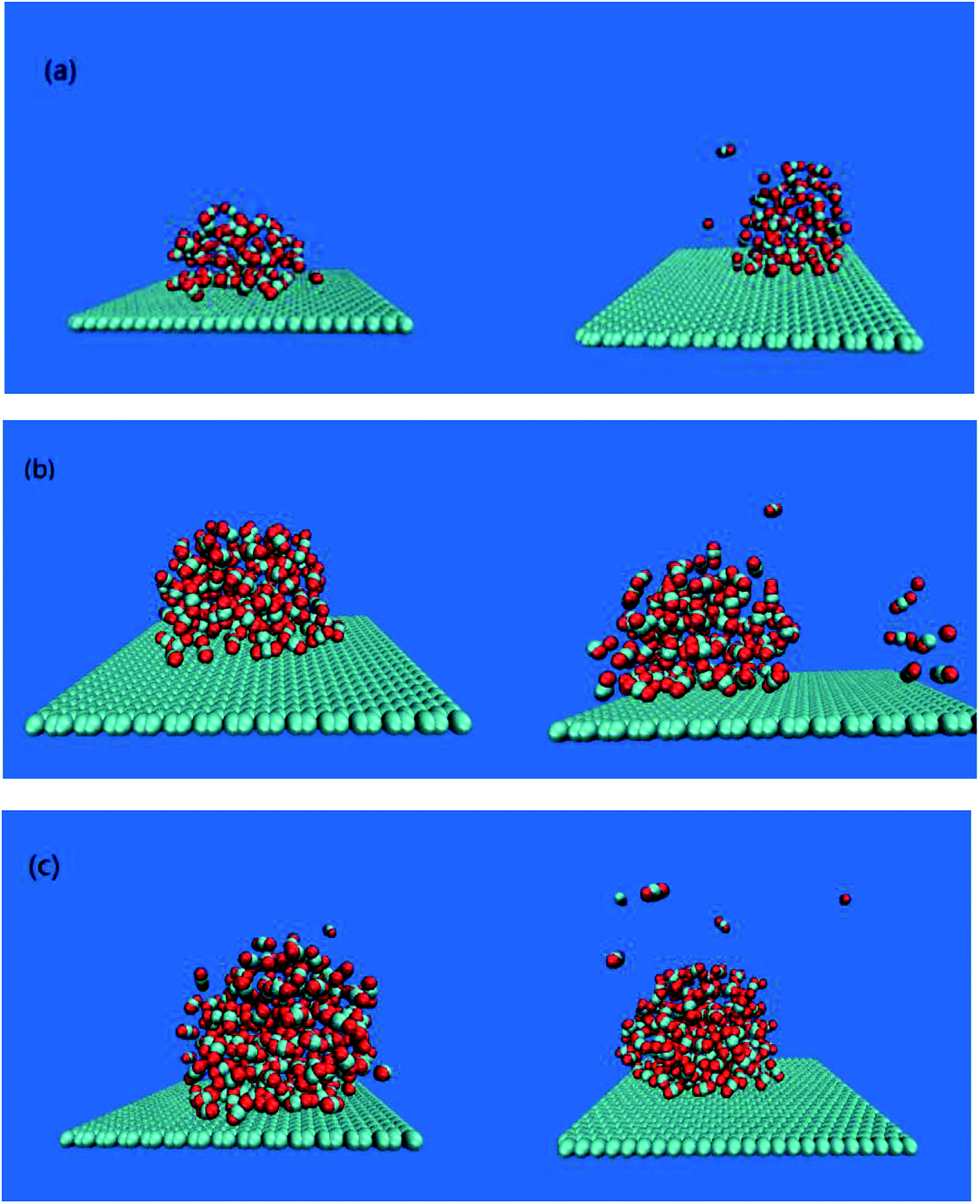 | ||
| Fig. 2 Snapshot of bubbles under different systems. (a), (b) and (c) are bubbles formed by a system containing 60, 120 and 180 CO2 molecules respectively, the left side is a bubble without an external electric field, and the right side is a bubble under an external electric field. | ||
It can be seen from Fig. 2 that different numbers of CO2 gas molecules form cylindrical bubbles. In order to study the change of bubble shape in the case of different dissolved gas volume without external electric field, the upper surface of graphene is defined as 0 nm, and the CO2 density profile along the z axis constructed by dividing the simulation box into small boxes with a desired thickness (0.05 nm) along the z axis. The calculated molecular density profile of CO2 gas is shown in Fig. 3. “60M”, “120M”, “180M” represent system models containing 60, 120 and 180 CO2 molecules, respectively.
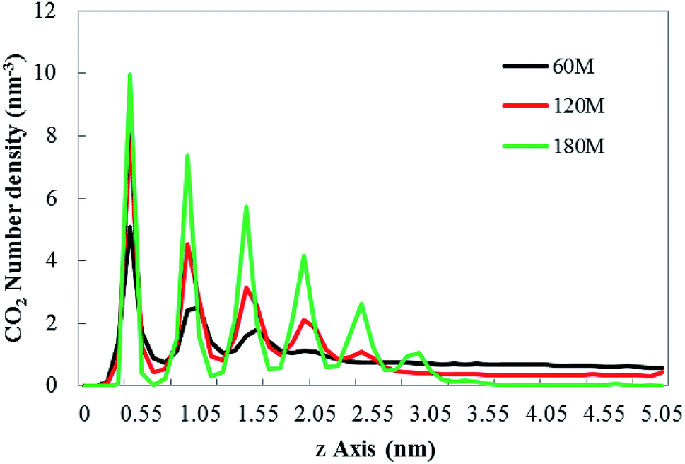 | ||
| Fig. 3 The CO2 density profile along the z axis under no external electric field. “60M”, “120M”, “180M” represent system models containing 60, 120 and 180 CO2 molecules in this paper, respectively. | ||
In Fig. 3, the abscissa represents the distance perpendicular to the graphene membrane (along the z-axis direction), the ordinate represents number density of CO2. Each peak of the curves indicates that in the relevant small box (with a desired thickness of 0.05 nm) the CO2 is present. The results show that the density profile of the gas consists of several peaks, which is consistent with the results of Hong's research.26 According to Fig. 3, as the gas content in the system increases, the height of the bubble with the hydrophobic substrate (the position at which the last peak is located) also increases.
The change of the bubble shape caused by the external electric field is reflected in the peak of the density profile. The numerical changes in the peak positions of the system containing the dissolved amounts of different gases are listed in Table 2.
| Position | 0.45 nm | 0.95 nm | 1.45 nm | 1.95 nm | 2.46 nm | |
|---|---|---|---|---|---|---|
| a “Position” represents the abscissa of each peak in CO2 density profile. | ||||||
| Without electric field | 60M | 5.09 | 2.52 | 1.82 | 1.10 | 0.76 |
| 120M | 8.00 | 4.54 | 2.82 | 1.75 | 0.77 | |
| 180M | 9.96 | 7.36 | 5.71 | 4.17 | 2.61 | |
| Under electric field | 60M | 5.00 | 2.39 | 1.80 | 1.10 | 0.76 |
| 120M | 7.89 | 4.35 | 2.80 | 1.76 | 0.78 | |
| 180M | 9.67 | 6.98 | 5.37 | 4.03 | 2.61 | |
The results in Table 2 show that the peak value of CO2 density profile under an external electric field is smaller than that without the electric field, and as the position away from the hydrophobic substrate is further, both peaks tend to be equal. In all systems in which CO2 molecules are dissolved, the decrease of the peak value means that the bubble size is smaller, the gas content inside the bubble becomes less, and a small amount of gas diffuses into the aqueous phase (as shown in Fig. 2(a)–(c)). Therefore, the results show that the size of bubbles is smaller when the electric field is applied in the process of air flotation, which promotes the combination of bubbles and hydrophobic particles and is beneficial to the adsorption and separation of hydrophobic particles by bubbles.
3.2 Self-diffusion coefficients
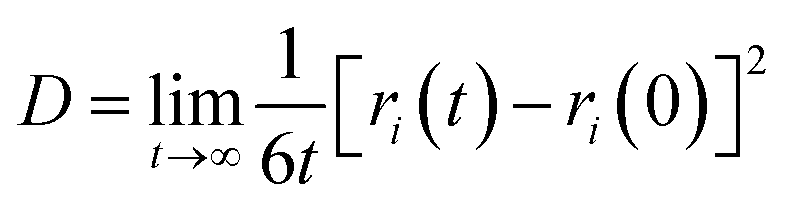
The diffusion coefficient is an important parameter of the gas in the aqueous solution, and it is a physical quantity that characterizes the gas diffusion ability. In this paper, the diffusion coefficient of CO2 is calculated using the “Einstein” relation:42
 | (1) |
Fig. 4 shows the self-diffusion coefficient of CO2 in systems with different amounts of gas dissolved under the external electric field and without an external electric field. It is known from Fig. 4 that the self-diffusion coefficient of CO2 becomes smaller and smaller with the increase of the dissolved amount of gas in the system regardless of whether or not an external electric field exists. When the amount of gas dissolved in the system is constant, the external electric field increases the self-diffusion coefficient of CO2 compared to that without an electric field. It is found from Fig. 3 that the contact radius of the bubble increases as the amount of dissolved gas increases. According to the Yang–Laplace equation,5 the larger the radius of the bubble leads to the smaller the internal pressure. Therefore, we conclude that the decrease of the internal pressure of the bubble is the main reason for the decrease of the self-diffusion coefficient of CO2 as the amount of dissolved gas increases. To investigate this phenomenon, we calculated the geometrical parameters (the inside pressure and the volume)43 of nanobubbles. It can be obtained from following equations:
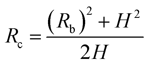 | (2) |
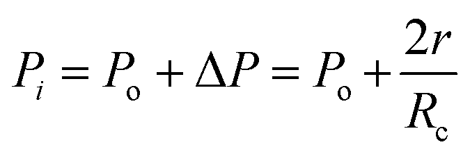 | (3) |
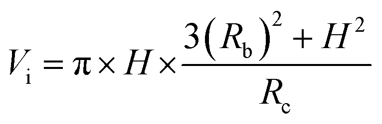 | (4) |
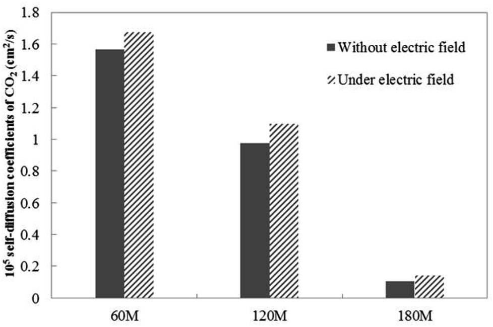 | ||
| Fig. 4 The CO2 self-diffusion coefficient of systems in which different amounts of gas molecules are dissolved without an external electric field and under an external electric field. | ||
The results are listed in Table 3
| H (nm) | Rb (nm) | P (atm) | V (nm3) | ||
|---|---|---|---|---|---|
| Without electric field | 60M | 1.95 | 0.85 | 1242.38 | 6.10 |
| 120M | 2.46 | 1.39 | 889.89 | 15.26 | |
| 180M | 2.97 | 1.38 | 797.58 | 22.60 | |
| Under electric field | 60M | 1.95 | 0.82 | 1253.17 | 5.94 |
| 120M | 2.46 | 1.35 | 901.00 | 14.83 | |
| 180M | 2.97 | 1.33 | 809.99 | 21.97 |
According to Table 3, we found that the bubble volume in the system increases as the amount of gas increases whether there is an external electric field or not. This result can meet with our conclusion that the increase of the amount of gas leads to the decrease of internal pressure of bubbles.
Under the external electric field, Fig. 4 shows that the diffusion coefficient of the gas becomes larger, so the fluidity of the gas inside the bubble becomes larger than when there is no external electric field. Therefore, we conclude that the increase of gas flow is the main reason for the bubble size becoming smaller. According to the dynamic equilibrium mechanism proposed by Lohse:24,44 the outflow of gas in the nanobubble and the inflow of gas will reach a dynamic equilibrium, and the outflow of the gas is proportional to the diffusion coefficient of the gas in the water. After reaching equilibrium, there will be a stable contact radius. During the air-floating process, the gas in the bubble is more active under the external electric field, the outflow of the gas in the bubble becomes larger, the contact radius of the bubble becomes smaller. The smaller bubble is more easily adsorbed on the hydrophobic particle.
3.3 Viscosity
Viscosity is a kinetic property that can affect the diffusion rate and conformational change of a molecule in an aqueous solution. The external electric field has an effect on the viscosity of the mixed system.45In this investigation, we used periodic perturbation method46 to calculate the viscosity of the system for nonequilibrium dynamic simulation. The Nose–Hoover extended ensemble for temperature coupling and the Parrinello–Rahman method for pressure coupling were used for calculating the viscosity. The viscosity (η) can be calculated with the aid of the following equation:
 | (5) |
 | (6) |
 | (7) |
Table 4 shows the viscosity of different systems. In Table 4, as the amount of dissolved gas increases, the viscosity also gradually increases. The viscosity value under the external electric field is lower than that without an external electric field. Normally, the diffusion coefficient of the solute in the solution is inversely related to the viscosity of the solution. The results in Table 4 are in good agreement with those in Fig. 4. Viscosity can be seen as an expression of internal friction in solution. As the amount of gas dissolved increases, the total attraction of the hydrophobic substrate to the gas molecules becomes greater, while more gas molecules also increases the friction with the water molecules. Therefore, the increase of the amount of gas dissolved leads to the increase of viscosity. When an external electric field is applied, some of the gas molecules in the bubble become more active, the gas molecules escaping from the bubble. They escape into the water phase, destroying the local hydrogen bond between the water molecules due to the movement of a small part of the gas,48–50 resulting in the decrease of viscosity. Under the external electric field, the decrease of viscosity promotes a small portion of the gas escaping from the bubble to be more easily recoupled with the hydrophobic particles in the aqueous phase to form a new bubble, thereby enhancing the effect of separating the hydrophobic solid particles by air flotation.
| Without electric field | Under electric field | |
|---|---|---|
| a “V60M”, “V120M”, “V180M” represent the viscosity of system with 60, 120, 180 CO2 molecules, respectively. | ||
| V60M (mPa s) | 0.0340 | 0.0336 |
| V120M (mPa s) | 0.0382 | 0.0378 |
| V180M (mPa s) | 0.0456 | 0.0452 |
3.4 Hydrogen bond
Hydrogen bonds between water molecules have a direct impact on the physical and chemical properties of solution system.51,52 Hydrogen bonding is a special state of connection of water molecules, because water molecules keep moving irregularly in solution, the rotation of water molecules (i.e., the increase in hydrogen bonding angle) destroys the hydrogen bonds that have formed.53 In this work we employed the geometrical hydrogen bond criterion which is widely used in MD simulation.54 It requires the oxygen–oxygen distance to be less than 3.5 Å and the H–O⋯O angle to be less than 30°. In order to reduce the numerical origin, the results of this parameter are obtained from the average of five repeated simulations.Fig. 5 shows that distribution of the hydrogen bond angle under an external electric field and without an external electric field. It can be seen that under no external electric field, the peak coordinates of the distribution of the hydrogen bond angle of systems with 60, 120, and 180 gas molecules are (9.5, 0.0554099), (9.5, 0.0545575) and (9.5, 0.0538870). The peak coordinates under an external electric field are (10.5, 0.0554477), (10.5, 0.0545804), (10.5, 0.0539568), respectively. Comparing the coordinates, it can be found that when there is an external electric field applied, the angle of the hydrogen bond generally becomes larger, and the rotation of the water molecule is more likely to break the original hydrogen bond. Thereby it causes a small part of the gas in the bubble easily escape to the water phase under the external electric field. When a part of the gas escapes from the bubble, the original hydrogen bond structure is destroyed, and the random movement of the water molecule is enhanced, which is consistent with the conclusion that the viscosity of the system is reduced under the external electric field.
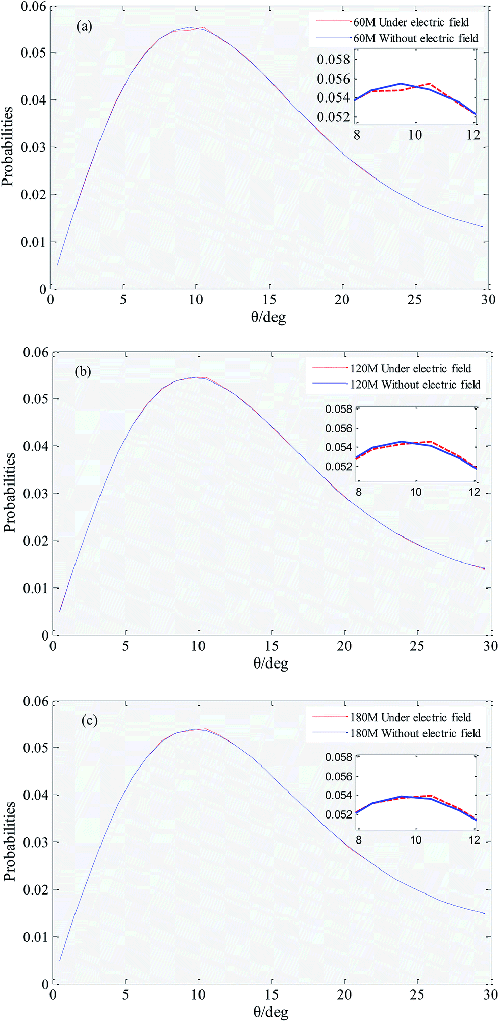 | ||
| Fig. 5 Distribution of the hydrogen bond angle. (a), (b) and (c) show the hydrogen bond angular distribution of systems with 60, 120, and 180 gas molecules, respectively, under an external electric field (red dashed line) and without an external electric field (blue solid line). | ||
Table 5 lists the proportion of water molecules containing 0–3 hydrogen bonds (f0 (%), f1 (%), f2 (%), f3 (%)). As can be seen from Table 5, regardless of whether or not an external electric field is applied, the proportion of water molecules (f0) that does not form hydrogen bonds decreases as the amount of dissolved gas increases, and the proportion of water molecules that form hydrogen bonds (f1, f2, f3) increases. Compared with that under no external electric field, f0 and f1 increase under the external electric field, while f2 and f3 decrease, indicating that the external electric field reduces the number of water molecules containing two and three hydrogen bonds, the binding between water molecules decrease. It may because that the external electric field makes the bubble size become smaller, and some gas molecules escape to water phase cause the change of the proportion of hydrogen bonds between water molecules.
| Without electric field | Under electric field | |||||||
|---|---|---|---|---|---|---|---|---|
| 0M | 60M | 120M | 180M | 0M | 60M | 120M | 180M | |
| f0 (%) | 39.65 | 39.89 | 39.71 | 39.59 | 39.50 | 39.90 | 39.73 | 39.60 |
| f1 (%) | 36.12 | 36.07 | 36.08 | 36.10 | 36.16 | 36.09 | 36.11 | 36.12 |
| f2 (%) | 19.61 | 19.50 | 19.58 | 19.65 | 19.67 | 19.49 | 19.56 | 19.64 |
| f3 (%) | 4.62 | 4.54 | 4.63 | 4.66 | 4.67 | 4.52 | 4.60 | 4.64 |
In addition, to clarity such changes are originated mostly by the presence of the CO2 molecules or by the electric field. The simulation that without CO2 molecules were also performed. The peak coordinate of hydrogen bond angle without an external electric field is (9.5, 0.0562010) and the peak coordinate of hydrogen bond angle under an external electric field is (9.5, 0.0562047) (figure or not given here). The results for fn were listed in Table 5 (0M), all the results show that the electric field enhanced the strength of the hydrogen bonds when there is no CO2 molecules existing in the system, which is consistent with Wei's work.55 But when there is CO2 molecules existing in the system, the results show that the electric field decreased the strength of the hydrogen bonds. Therefore, the results show that the changes are originated mostly by the electric field.
4. Conclusions
In this paper, molecular dynamics simulation was used to investigate the effect of external electric field on nanobubbles adsorbed at the surface of hydrophobic particles, and compared with results under no external electric field, some important conclusions are obtained:(1) The results show that the size of bubbles is smaller when there is an external electric field applied. The smaller size of bubbles is beneficial to promoting the combination of bubbles and hydrophobic particles in the process of air flotation.
(2) As the amount of gas in the system increases, the diffusion coefficient of the gas molecules gradually decreases, which may be caused by the decrease of the internal pressure of the bubbles. The external electric field makes the gas molecules more active, and some of the gas molecules escape from the bubbles and escape to the water phase away from the hydrophobic substrate, so that the size of the bubbles under the external electric field become smaller.
(3) External electric field will reduce the viscosity of the system, when the bubble size becomes smaller, a small amount of gas escaped from the bubble will destroy the hydrogen bond structure in aqueous solution. Compared with that under no external electric field, the external electric field makes the angle of hydrogen bond between water molecules larger, the hydrogen bond is easier to be destroyed, and the proportion of water molecules with more hydrogen bonds decreases, and the hydrogen bond binding between water molecules weakens.
Conflicts of interest
There are no conflicts to declare.Acknowledgements
This work was financially supported by the National Natural Science Foundation of China (Grant No. 51408525).References
- J. L. Parker, P. M. Claesson and P. Attard, J. Phys. Chem., 1994, 98, 8468–8480 CrossRef CAS.
- L. Zhang, Y. Zhang and X. Zhang, Langmuir, 2006, 22, 8109–8113 CrossRef CAS PubMed.
- M. A. Hampton and A. V. Nguyen, Adv. Colloid Interface Sci., 2010, 154, 30–55 CrossRef CAS PubMed.
- S. Karpitschka, E. Dietrich and J. R. T. Seddon, Phys. Rev. Lett., 2012, 109, 066102 CrossRef PubMed.
- V. S. J. Craig, Soft Matter, 2011, 7, 40–48 RSC.
- C. Chan, L. Chen and M. Arora, Phys. Rev. Lett., 2015, 114, 114505 CrossRef PubMed.
- T. Ito, H. Lhuissier and S. Wildeman, Phys. Fluids, 2014, 26, 032003 CrossRef.
- V. S. Ajaev, Phys. Fluids, 2006, 18, 068101 CrossRef.
- N. Kameda, N. Sogoshi and S. Nakabayashi, Surf. Sci., 2008, 602, 1579–1584 CrossRef CAS.
- J. R. T. Seddon, H. J. W. Zandvliet and D. Lohse, Phys. Rev. Lett., 2011, 107, 116101 CrossRef PubMed.
- W. A. Ducker, Langmuir, 2009, 25, 8907–8910 CrossRef CAS PubMed.
- Y. Liu and X. Zhang, J. Chem. Phys., 2013, 138, 014706 CrossRef PubMed.
- D. Tao, S. Yu and X. Zhou, Int. J. Coal Prep. Util., 2008, 28, 1–14 CrossRef CAS.
- Y. J. Tao, J. T. Liu and S. Yu, Sep. Sci. Technol., 2006, 41, 16 CrossRef.
- M. A. Hampton and A. V. Nguyen, Miner. Eng., 2009, 22, 786–792 CrossRef CAS.
- M. M. Fan, T. Daniel and R. Honaker, Int. J. Min. Sci. Technol., 2010, 20, 1–19 CAS.
- Y. Han, C. Zhang and L. Wu, J. Cryst. Growth, 2018, 499, 67–76 CrossRef CAS.
- N. Li, S. Tang and Y. Rao, Electrochim. Acta, 2018, 270, 330–338 CrossRef CAS.
- L. Zhu and Y. Han, J. Mol. Liq., 2018, 271, 820 CrossRef CAS.
- J. M. Thiebaut, J. P. Vaubourg and G. Roussy, J. Phys. D: Appl. Phys., 1989, 22, 154 CrossRef CAS.
- M. Birinci, J. D. Miller and M. Sarıkaya, Miner. Eng., 2010, 23, 813–818 CrossRef CAS.
- M. Murugananthan, G. B. Raju and S. Prabhakar, Sep. Purif. Technol., 2004, 40, 69–75 CrossRef CAS.
- C. Li, A. Zhang and S. Wang, AIP Adv., 2018, 8, 015104 CrossRef.
- J. H. Weijs, J. H. Snoeijer and D. Lohse, Phys. Rev. Lett., 2012, 108, 104501 CrossRef PubMed.
- H. J. C. Berendsen, J. R. Grigera and T. P. Straatsma, J. Phys. Chem., 1987, 91, 6269 CrossRef CAS.
- P. Hong, G. R. Birkett and A. V. Nguyen, Langmuir, 2013, 29, 15266–15274 CrossRef PubMed.
- L. Wang, X. Wang and L. Wang, Nanoscale, 2017, 9, 1078 RSC.
- J. Li and F. Wang, J. Chem. Phys., 2017, 146, 054702 CrossRef PubMed.
- J. G. Harris and K. H. Yung, J. Phys. Chem., 1995, 99, 12021 CrossRef CAS.
- X. Li, D. A. Ross and J. P. M. Trusler, J. Phys. Chem. B, 2013, 117, 5647 CrossRef CAS PubMed.
- H. Jiang, I. G. Economou and A. Z. Panagiotopoulos, Acc. Chem. Res., 2017, 50, 751 CrossRef CAS PubMed.
- W. L. Jorgensen, D. S. Maxwell and J. Tirado-Rives, J. Am. Chem. Soc., 1996, 118, 11225 CrossRef CAS.
- D. S. D. Van, E. Lindahl and B. Hess, J. Comput. Chem., 2005, 26, 1701–1718 CrossRef PubMed.
- R. E. Iseleholder, W. Mitchell and A. E. Ismail, J. Chem. Phys., 2012, 137, 1133 Search PubMed.
- A. M. Saitta, F. Saija and P. V. Giaquinta, Phys. Rev. Lett., 2012, 108, 207801 CrossRef PubMed.
- Q. G. Jiang, Z. M. Ao and D. W. Chu, J. Phys. Chem. C, 2012, 116, 19321 CrossRef CAS.
- P. Hong, M. A. Hampton and A. V. Nguyen, Langmuir, 2013, 29, 6123–6130 CrossRef PubMed.
- Y. H. Lu, C. W. Yang and I. S. Hwang, Langmuir, 2012, 28, 12691–12695 CrossRef CAS PubMed.
- L. Zhang, X. Zhang and C. Fan, Langmuir, 2009, 25, 8860–8864 CrossRef CAS PubMed.
- X. H. Zhang, X. Zhang and J. Sun, Langmuir, 2006, 23, 1778–1783 CrossRef PubMed.
- M. C. Zaghdoudi and M. Lallemand, Int. J. Therm. Sci., 2000, 39, 39–52 CrossRef.
- P. Henritzi, A. Bormuth and F. Klameth, J. Chem. Phys., 2015, 143, 164502 CrossRef PubMed.
- D. Y. Li, D. L. Jing and Y. L. Pan, Langmuir, 2014, 30, 6079 CrossRef CAS PubMed.
- M. P. Brenner and D. Lohse, Phys. Rev. Lett., 2008, 101, 214505 CrossRef PubMed.
- B. Hess, J. Chem. Phys., 2002, 116, 209–217 CrossRef CAS.
- L. Zhao, T. Cheng and H. Sun, J. Chem. Phys., 2008, 129, 144501 CrossRef PubMed.
- L. Zhu, Y. Han and C. Zhang, RSC Adv., 2017, 7, 47583–47591 RSC.
- V. S. J. Craig, B. W. Ninham and R. M. Pashley, Nature, 1993, 364, 317–319 CrossRef CAS.
- P. K. Weissenborn and R. J. Pugh, J. Colloid Interface Sci., 1996, 184, 550–563 CrossRef CAS PubMed.
- C. L. Henry, J. Phys. Chem. C, 2006, 111, 1015–1023 CrossRef.
- W. J. Lee, J. G. Chang and S. P. Ju, Langmuir, 2010, 26, 12640–12647 CrossRef CAS PubMed.
- Z. Pan, J. Chen and G. Lü, J. Chem. Phys., 2012, 136, 164313 CrossRef PubMed.
- H. S. Lee and M. E. Tuckerman, J. Chem. Phys., 2006, 125, 154507 CrossRef PubMed.
- X. Zhang, Q. Zhang and D. X. Zhao, Acta Phys.-Chim. Sin., 2011, 27, 2547–2552 CAS.
- S. Wei, C. Zhong and H. Su-Yi, Mol. Simul., 2005, 31, 555–559 CrossRef CAS.
| This journal is © The Royal Society of Chemistry 2019 |