
Energy-based descriptors to rapidly predict hydrogen storage in metal–organic frameworks†
Benjamin J.
Bucior
 a,
N. Scott
Bobbitt
a,
Timur
Islamoglu
b,
Subhadip
Goswami
b,
Arun
Gopalan
a,
Taner
Yildirim
c,
Omar K.
Farha
ab,
Neda
Bagheri
*ad and
Randall Q.
Snurr
*a
a,
N. Scott
Bobbitt
a,
Timur
Islamoglu
b,
Subhadip
Goswami
b,
Arun
Gopalan
a,
Taner
Yildirim
c,
Omar K.
Farha
ab,
Neda
Bagheri
*ad and
Randall Q.
Snurr
*a
aDepartment of Chemical and Biological Engineering, Northwestern University, Evanston, IL 60208, USA. E-mail: n-bagheri@northwestern.edu; snurr@northwestern.edu
bDepartment of Chemistry, Northwestern University, Evanston, IL 60208, USA
cNIST Center for Neutron Research, National Institute of Standards and Technology, Gaithersburg, MD 20899, USA
dCenter for Synthetic Biology, Northwestern University, Evanston, IL 60208, USA
First published on 1st November 2018
Abstract
The low volumetric density of hydrogen is a major limitation to its use as a transportation fuel. Filling a fuel tank with nanoporous materials, such as metal–organic frameworks (MOFs), could greatly improve the deliverable capacity of these tanks if appropriate materials could be found. However, since MOFs can be made from many combinations of metal nodes, organic linkers, and functional groups, the design space of possible MOFs is enormous. Experimental characterization of thousands of MOFs is infeasible, and even conventional molecular simulations can be prohibitively expensive for large databases. In this work, we have developed a data-driven approach to accelerate materials screening and learn structure–property relationships. We report new descriptors for gas adsorption in MOFs derived from the energetics of MOF–guest interactions. Using the bins of an energy histogram as features, we trained a sparse regression model to predict gas uptake in multiple MOF databases to an accuracy within 3 g L−1. The interpretable model parameters indicate that a somewhat weak attraction between hydrogen and the framework is ideal for cryogenic storage and release. Our machine learning method is more than three orders of magnitude faster than conventional molecular simulations, enabling rapid exploration of large numbers of MOFs. As a case study, we applied the method to screen a database of more than 50![[thin space (1/6-em)]](https://www.rsc.org/images/entities/char_2009.gif) 000 experimental MOF structures. We experimentally validated one of the top candidates identified from the accelerated screening, MFU-4l. This material exhibited a hydrogen deliverable capacity of 47 g L−1 (54 g L−1 simulated) when operating at storage conditions of 77 K, 100 bar and delivery at 160 K, 5 bar.
000 experimental MOF structures. We experimentally validated one of the top candidates identified from the accelerated screening, MFU-4l. This material exhibited a hydrogen deliverable capacity of 47 g L−1 (54 g L−1 simulated) when operating at storage conditions of 77 K, 100 bar and delivery at 160 K, 5 bar.
Design, System, ApplicationMetal–organic frameworks (MOFs) have high internal surface area and internal porosity, which makes them good candidates for gas storage applications. MOFs are synthesized in a “building-block” approach from metal nodes and organic linkers, which enables tailored chemistries and geometries for specific applications. However, the enormous number of building blocks and topologies makes it challenging to select the best material for a given application. Grand canonical Monte Carlo (GCMC) simulations can accurately characterize adsorption properties, but brute force screening of MOF structure databases is prohibitively expensive. In this work we applied feature engineering and machine learning to accelerate MOF screening and design. The new descriptor is inspired by the thermodynamics of adsorption, so it is accurate, transferable, and provides insight into MOF design principles. We used the model to filter a database containing >50000 experimental MOF structures by estimating gas uptake. We focused GCMC simulations on the top 1% of them and selected one highly promising MOF for experimental synthesis and characterization. The material identified in this work is potentially suitable for fuel storage in hydrogen-powered vehicles. Future use of this general approach may accelerate MOF design for other applications in gas storage and separations.
|
1 Introduction
Efficient, reliable energy storage is one of the most difficult challenges in transitioning from reliance on fossil fuels to a more sustainable energy economy. Designing energy storage systems for the transportation sector is especially challenging due to portability requirements and size and weight constraints for passenger vehicles. Hydrogen is an appealing option for transportation energy storage because it is nontoxic and its oxidation product is environmentally benign water vapor. In recent years, several major automobile manufacturers—including Honda, Toyota, Hyundai, and General Motors1–4—have been developing hydrogen-powered vehicles. There are an estimated 3000 hydrogen fuel cell vehicles currently operating in the United States.5 Also, the French rail company Alstom recently announced a hydrogen fuel cell passenger train that will soon be launched in Germany.6Most of these vehicles currently store compressed hydrogen around 700 bar and at ambient temperature; however, storing gas at such a high pressure involves safety concerns that require special consideration, such as thick-walled tanks, hoses, and other components. There has recently been significant interest in storing hydrogen at lower pressures using cryo-adsorption in which the hydrogen is adsorbed to a porous material at cryogenic temperature.7,8 The density of adsorbed hydrogen – and thus the storage capacity – is dramatically higher at 77 K (the temperature of liquid nitrogen) than at 300 K (hydrogen gas density at 1 bar, 77 K is 0.315 g L−1vs. 0.081 g L−1 at 1 bar, 300 K). For example, in ZIF-8, hydrogen uptake is 3.3 wt% (3.3 g H2 per 100 g MOF) at 77 K and 30 bar, but is only 0.13 wt% at 298 K and 60 bar.9 In IRMOF-1 (MOF-5) the hydrogen uptake is 4.7 wt% at 77 K and 50 bar but it is only 0.28 wt% at 298 K and 65 bar.10 The United States Department of Energy (DOE) has defined hydrogen storage goals that adsorbent materials should reach in order to be integrated into a commercially viable vehicle with an acceptable driving range. The current goals are to reach 4.5 wt% and 30 g L−1 by 2020, with ultimate goals of 6.5 wt% and 50 g L−1. For context, the density of liquid hydrogen at 1 bar and 20.3 K is 70.9 g L−1. There has been significant scientific effort devoted to hydrogen storage in porous materials in the last few years;11–17 however, no existing material currently meets DOE targets at ambient temperature.
Metal–organic frameworks (MOFs) are a class of crystalline materials that are highly porous and have high specific surface areas, which make them attractive candidates for applications in gas storage and separations.18–20 MOFs are made from inorganic nodes (often metal or metal oxide clusters) connected by organic linkers.21 These linkers can be decorated with different functional groups to modify the MOF's chemical and physical properties.22 There are many different nodes, linkers, and functional groups that can be combined in different topological nets.23 MOFs can also be modified post-synthetically by adding more functional groups or substituting metal atoms in the node.24 This means there are virtually an unlimited number of combinations of nodes, linkers, functional groups, and topologies representing an infinite number of possible MOFs. Chung et al. published 5109 porous structures that have successfully been synthesized in the computation-ready, experimental (CoRE) MOF database.25 The Cambridge Crystallographic Data Centre (CCDC) has published a set of 69666 structures that fit their criteria for being considered MOFs,26 although we note that many of the structures in this database are nonporous. Hundreds of thousands more MOFs have been predicted theoretically but have not yet been synthesized.27–29
There are far more possible MOFs than could reasonably be synthesized and characterized experimentally. High-throughput computational methods can screen tens of thousands of structures quickly to identify promising candidates for a specific application. Many groups have used computational screening to study MOFs for methane storage,27,30–32 hydrogen storage,33–36 CO2 capture,37,38 and other applications.39–44 Many of these studies use grand canonical Monte Carlo (GCMC) simulations to calculate uptake of the target molecule. However, even efficient GCMC simulation techniques require substantial computational time and effort for a large number of structures. Computing the uptake at high pressure for a single MOF can take days or even weeks. In order to reduce the computational expense for large-scale screening, some groups have recently been working on low cost algorithms to estimate the performance of MOFs for gas storage and to replace brute force GCMC screening of hundreds of thousands of materials. Siegel et al. validated an empirical correlation, the Chahine rule,45,46 between surface area and hydrogen uptake at 35 bar for 5309 MOFs.47 We have previously reported a simple metric called the binding fraction that can be computed quickly from a MOF's geometry to provide its suitability for hydrogen storage.35
Others have reduced the number of necessary GCMC simulations by judiciously sampling the design space of MOF structures. For example, Chung et al. used a genetic algorithm to efficiently search a large database of MOFs for top-performing CO2 sorbents.38
Machine learning methods have also been emerging as a way to prescreen materials and accelerate large-scale simulation workflows. Textural properties such as the pore volume and surface area are the most common descriptors for structure–property relationships in MOFs.27,31,48 Supervised learning methods can utilize these geometric properties to predict gas uptake in MOFs and highlight the most important features for future design.39,49–51 For example, researchers applied artificial neural networks to study hydrogen storage in a diverse materials database containing over 850000 materials.33 There is considerable opportunity to diversify the type of descriptors beyond the standard set of textural properties.52 Some machine learning studies have considered chemical properties in addition to the classic textural set,53 and some have developed novel chemical features.28,54 Different definitions or methods of calculating pore descriptors (i.e. energetic vs. geometric criteria) are also being revisited in the literature.55,56
High-throughput screening is effective at identifying the best candidates for a given storage or separation application. However, these calculations also produce vast quantities of data that are currently being underutilized. Machine learning and data mining techniques offer great potential not only to accelerate materials simulations but also to glean deeper insights into structure-performance trends. For example, in our previous work35 we identified the optimal pore diameter, void fraction, and linker geometry of top-performing MOFs for cryogenic hydrogen storage. However, the relationship between textural properties and hydrogen storage is complex, and it is difficult to evaluate a MOF's capacity based on a single property. A high void fraction is generally beneficial, but there is an optimal value beyond which a larger void fraction is detrimental. The case is the same for pore diameter, and the relationship between deliverable capacity and gravimetric and volumetric measures of surface area is unclear.35 In this work, we demonstrate a way to reduce this complexity down to a single figure-of-merit, which directly correlates with hydrogen capacity and does not require textural properties as inputs. Our new descriptor uses the potential energy landscape of a MOF to predict gas storage at very low computational cost yet with high predictive accuracy. We also demonstrate that this method is quite general and transferable to other gases and diverse MOF families.
2 Methods
2.1 Data collection
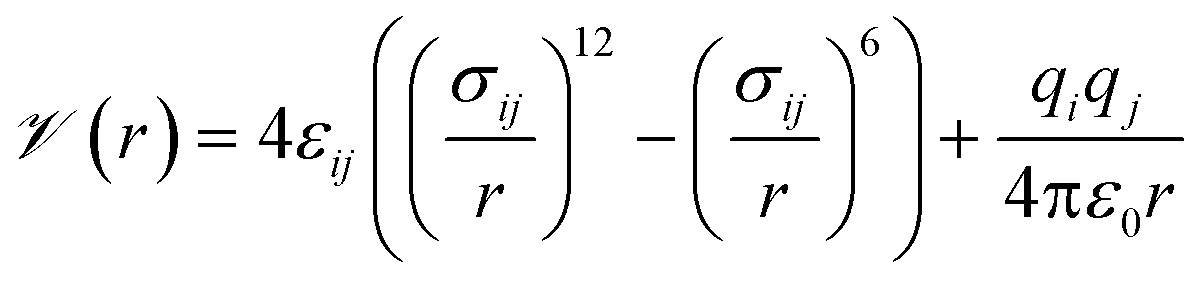
Our general approach was to apply supervised learning methods to predict a MOF's volumetric deliverable capacity for hydrogen by using information from its three-dimensional potential energy landscape. The model was able to accelerate screening by rapidly narrowing down the list of candidate MOFs selected for full GCMC simulations. In this subsection, we discuss the sources of data used in the machine learning analysis. We begin with the simulation methodology and parameters for adsorption calculations, then describe details for an experimental confirmation.The energetics of adsorption are commonly modeled using interatomic potentials. Throughout our simulations, we assumed a rigid MOF structure with atoms that interact with adsorbates through Lennard-Jones plus Coulombic potentials:
 | (1) |
![[scr V, script letter V]](https://www.rsc.org/images/entities/char_e149.gif) is the potential energy between atoms i and j that are a distance r apart, ε and σ are the Lennard-Jones parameters, and qi is the partial charge on atom i. We took the Lennard-Jones parameters for the framework atoms from the Universal Force Field58 and applied the Lorentz–Berthelot mixing rules for cross terms. We represented hydrogen using a rigid, three-site model with the H–H bond length fixed at 0.741 Å. The center of mass site used Lennard-Jones parameters from the model of Michels–Degraaff–Tenseldam59 of σ = 2.958 Å and ε/kB = 36.7 K; there are no Lennard-Jones interactions for the other two sites. All three sites had partial charges from the Darkrim–Levesque model: q = 0.468e on the H nuclei and q = −0.936e at the center of mass.60 We did not assign partial charges to the framework atoms, so H2–framework electrostatic interactions were neglected. We modified the H2–H2 and H2–framework Lennard-Jones interactions with the Feynman–Hibbs correction61 to account for quantum effects, which are important at cryogenic temperatures (Fig. S12†), resulting in the potential
is the potential energy between atoms i and j that are a distance r apart, ε and σ are the Lennard-Jones parameters, and qi is the partial charge on atom i. We took the Lennard-Jones parameters for the framework atoms from the Universal Force Field58 and applied the Lorentz–Berthelot mixing rules for cross terms. We represented hydrogen using a rigid, three-site model with the H–H bond length fixed at 0.741 Å. The center of mass site used Lennard-Jones parameters from the model of Michels–Degraaff–Tenseldam59 of σ = 2.958 Å and ε/kB = 36.7 K; there are no Lennard-Jones interactions for the other two sites. All three sites had partial charges from the Darkrim–Levesque model: q = 0.468e on the H nuclei and q = −0.936e at the center of mass.60 We did not assign partial charges to the framework atoms, so H2–framework electrostatic interactions were neglected. We modified the H2–H2 and H2–framework Lennard-Jones interactions with the Feynman–Hibbs correction61 to account for quantum effects, which are important at cryogenic temperatures (Fig. S12†), resulting in the potential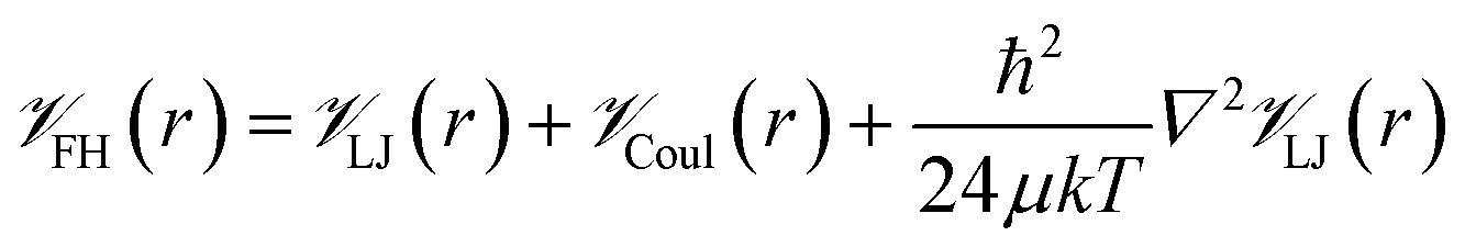 | (2) |
Methane was represented as a single-site pseudo atom using the TraPPE force field.62 Lennard-Jones interactions were truncated with a cutoff of 12.8 Angstroms. We were able to reduce the required computation time for this study by reusing some GCMC simulation data from previous work on cryogenic hydrogen adsorption in hMOFs.35 The statistical errors for the GCMC simulations for the CCDC MOFs are given in Table S3.†
953 hypothetical MOFs (denoted “hMOFs” herein) by geometrically assembling MOF building blocks and functional groups with a “bottom-up” construction algorithm.27 Colón, Gómez-Gualdrón, and coworkers computationally assembled 13512 topologically diverse MOFs using their topologically based crystal constructor (ToBaCCo) code, which uses a “top-down” algorithm to position MOF building blocks onto topological blueprints.29,36 Finally, we considered experimental structures aggregated in the CCDC MOF subset.26 High-performing structures from the CCDC database would be especially interesting since there are existing synthesis protocols. We started with non-disordered structures and removed all solvent molecules using the Python scripts provided in the ESI† of the CCDC MOF paper,26 which simulates the fully activated structures. We then converted the CIFs to P1 symmetry using Materials Studio to simplify symmetry operations.63 After processing, 54776 structures were successfully extracted.
Surprisingly, a somewhat coarse 1.0 Angstrom grid spacing is sufficient for our analysis (section 3.1). For most MOFs, the calculated energy histogram bins are consistent between a 1.0 Angstrom grid and a finer 0.5 Angstrom spacing (Fig. S31†). Training the model on the finer 0.5 Angstrom grid spacing slightly increases the accuracy of the predictions (Fig. S30†), but the increased grid resolution may not warrant the increased computation time, which scales as (1/spacing3). Based on this tradeoff, we prioritized calculation speed, because we intended to rapidly screen large MOF databases and identify leads to study with more detailed simulations.
Fig. 1 summarizes our workflow for feature extraction and model calculations. Many machine learning methods require a fixed number of input variables, so we converted the 3D energy landscape into a 1D distribution by taking a histogram binned by energy. This transformation makes the approximation that all sites with the same energy have similar adsorption properties, so spatial details (i.e. relative positioning of the sites) are discarded. In the energy histogram, the height of each bin represents the proportion of the unit cell with a particular host–guest interaction energy. For example, one bin reports the proportion of grid points with an energy between −5 kJ mol−1 and −4 kJ mol−1 of attraction. Since each bin represents a probability, the sum over all bins for a given MOF is unity.
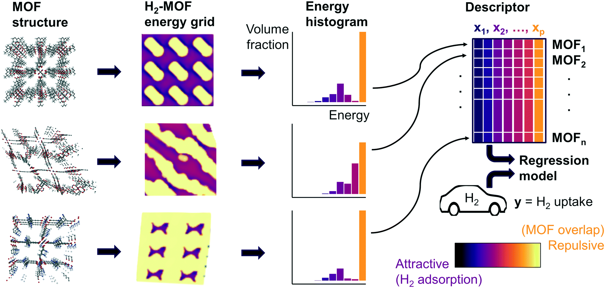 | ||
| Fig. 1 Overall machine learning workflow. For each MOF, we sampled the potential energy distribution by calculating the energy of a hydrogen probe at grid points within the MOF unit cell, then summarized the distribution of energies as a histogram. Each bin in the resulting energy histogram is a feature in the regression model, which enables the model to capture effects from different attractive and repulsive regions of the MOF in predicting hydrogen deliverable capacity. | ||
For hydrogen, we calculated bins using a width of 1 kJ mol−1 ranging from −10 kJ mol−1 (attractive) to 0 kJ mol−1. Geometric overlap between a grid point and MOF atom is a (highly) repulsive interaction, so we included a single bin for all positive values of energy.
Some grid points have a greater attractive energy than the −10 kJ mol−1 bound, so we likewise included a bin for energies less than −10 kJ mol−1 (see Table S5†). Energy grids for methane were calculated similarly. Since methane adsorbs more strongly than hydrogen, we generated bins in 2 kJ mol−1 increments between −26 and 0 kJ mol−1, again with a repulsion bin. More details about the histogram calculations are discussed in section 3.2.
2.2 Data analysis
Our supervised learning method analyzes the energy and GCMC data discussed in the previous section. The response variable we are trying to predict is the hydrogen deliverable capacity for a MOF. The feature matrix consists of n MOFs and p explanatory variables, which are the histogram bins for each MOF. For example, the selected histogram parameters for hydrogen yield an energy histogram containing 12 bins for each MOF. Thus, the feature matrix for the hMOFs has dimensions 137953 by 12.
We tested several forms of linear regression to correlate the energy histogram bins to gas uptake in MOFs. The simplest is multiple linear regression (MLR), a multidimensional generalization of ordinary least squares linear regression. The model is fit with a linear coefficient βj for each explanatory variable xj, plus the y-intercept β0 and takes the form
| y = βX = β0 + β1x1 + β2x2 + ⋯ + βpxp. | (3) |
In this work, we primarily used a sparse linear regression algorithm: least absolute shrinkage and selection operator (LASSO) regression.64 The final model takes the same form as MLR, but the β coefficients are fit differently. In MLR and simple linear regression, the goal is to minimize the sum of squared errors from the residuals. LASSO modifies the objective function by adding a penalty term based on the L1-norm of the coefficients (the sum of their absolute values). In LASSO, the strength of this penalty term is set by a hyperparameter λ, so the training algorithm solves for the β coefficients that minimize the following argument.
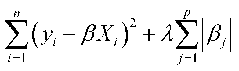 | (4) |
If λ is set to zero, then the objective function reduces to MLR. In general, adding a penalty term while training machine learning models is called regularization, and it helps avoid overfitting a model to the training data by balancing the fitting accuracy against the model simplicity. LASSO in particular is an effective method for feature selection since it can set coefficients to zero, thus generating a sparse model.
We carried out data analysis in R65 using the glmnet66 package for model calculations. To assess the accuracy of model predictions, we used simple random sampling to divide each database into 1000 MOFs for model training and a set of different MOFs as separate holdout data for testing. We set the regularization parameter λ using an automated approach in the glmnet package, described in Fig. S22.† The fitting procedure in this package implicitly standardizes the explanatory variables by fitting a model using the z-score of each variable, then it transforms the model β coefficients back to the original units so the fitted equation can be used as-is with the original, unstandardized variables.
2.3 Experimental details
A published procedure was followed for the synthesis of MFU-4l.67 The MOF crystals were recovered by centrifuge, washed with dimethylformamide, methanol, and dichloromethane and then soaked in dichloromethane overnight. The solvent exchanged MOF crystals were then activated under vacuum at 180 °C for 18 h prior to gas adsorption measurements. Gas isotherm measurements were performed on a carefully calibrated, high accuracy, Sieverts apparatus under computer control at NIST. The instrument and measurement-protocol are described in detail by Peng et al.68 For further details, refer to the ESI.†3 Results and discussion
3.1 Model interpretation and performance
Prior work on a “binding fraction” metric pointed out an optimum binding strategy for hydrogen storage via physisorption at cryogenic conditions.35 A material needs to have sufficient hydrogen–framework interactions to bind hydrogen; otherwise its void space will have relatively low hydrogen density even at high pressure. However, if the material binds hydrogen too strongly, the gas cannot be released. Thus, even though a strongly adsorbing site increases the absolute uptake of hydrogen at storage conditions, it does not contribute to deliverable capacity unless hydrogen can also desorb at the lower delivery pressure. The balance of adsorption strength is demonstrated in Fig. 2, which highlights two examples of MOFs with different adsorption and uptake properties.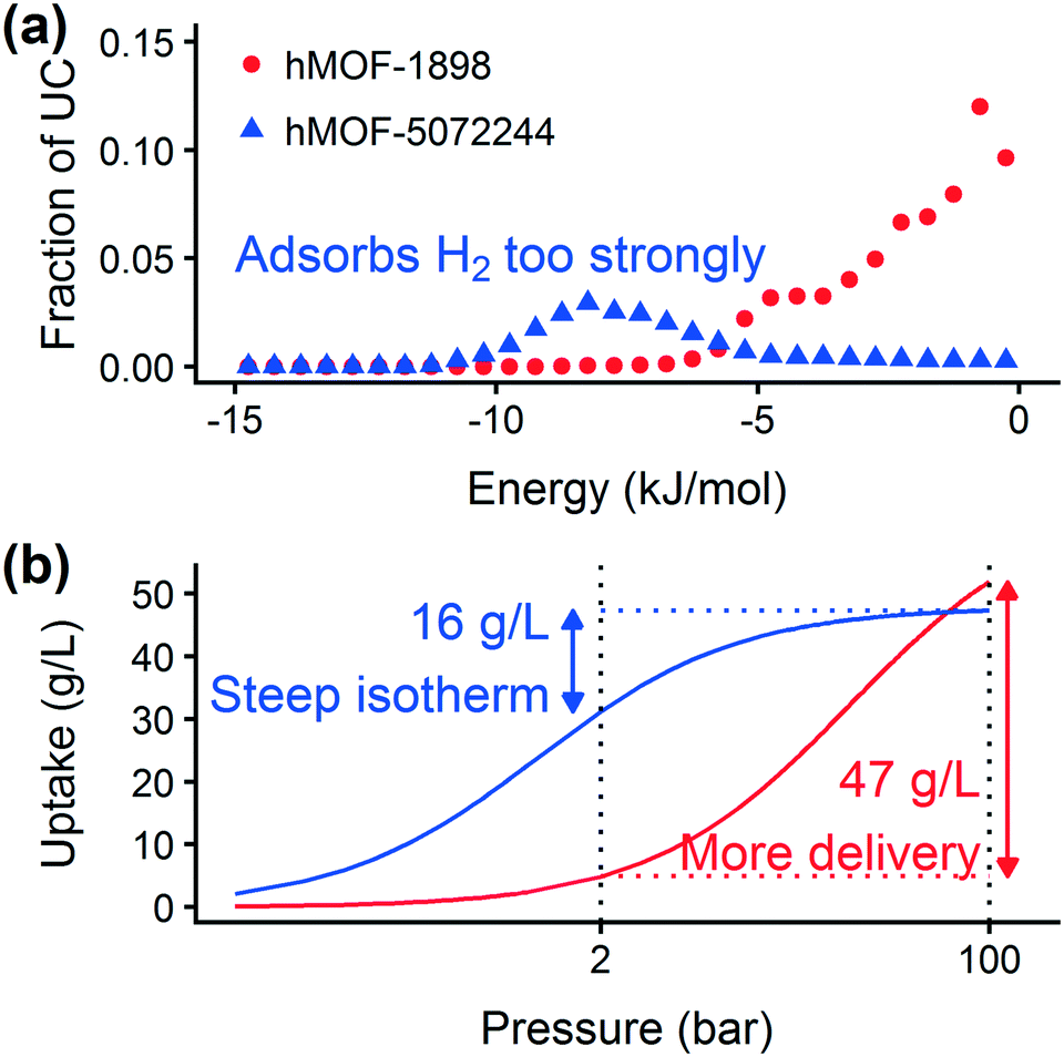 | ||
| Fig. 2 (a) Case study of two MOFs, hMOF-1898 and hMOF-5072244, with different pore energetics. (b) Although the MOFs have similar saturation loadings, their deliverable capacity is considerably different due to the amount of hydrogen remaining in the tank at low pressure. Dashed lines designate the delivery and storage pressures of 2 bar and 100 bar, respectively. The x-axis is plotted on a log scale. | ||
In order to capture the effects of adsorption strength, we developed a descriptor derived from the energy distribution (discussed in section 2.1.3 and Fig. 1). The gray points in Fig. 3(a) depict the coefficients for the LASSO model. We fit the model β coefficients by training the model against GCMC hydrogen deliverable capacity for 1000 structures in the hMOF database. An example energy histogram (MOF-5) is depicted by the bars in Fig. 3(a): we can predict the hydrogen deliverable capacity for this MOF by multiplying each β coefficient by the height of the corresponding histogram bar, then taking the sum of these contributions and the β0 constant term. See eqn (3).
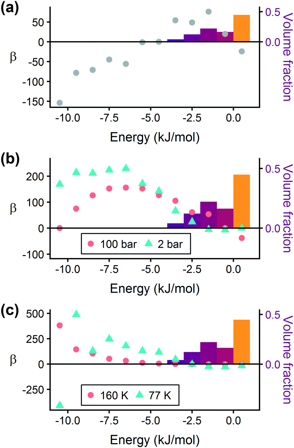 | ||
| Fig. 3 Regression coefficients, drawn as points, overlaid on the energy histogram for MOF-5. Histogram bars are shaded using the same color bar as Fig. 1. Points represent the β coefficients for the LASSO regression model trained on GCMC data for 1000 hMOFs. The model is fit to hydrogen adsorption data calculated (a) as the deliverable capacity between 100 bar and 2 bar at 77 K, (b) separately at pressures of 2 bar and 100 bar at 77 K, and (c) at two different temperatures of 160 K and 77 K at 2 bar. The deliverable capacity β values are provided in Table S6.† | ||
Examining Fig. 3(a) from right to left, we first note that the strongly repulsive region has a negative β coefficient. The negative coefficient means that if the MOF were modified in a way that increased this histogram bin (in this case, by adding to the repulsive region of the MOF), the deliverable capacity would decrease. Specifically for this bin, more space would be occupied by framework atoms, leaving less void space available for hydrogen adsorption. In contrast, the weakly attractive region from −4 kJ mol−1 to 0 kJ mol−1 has the largest positive β coefficients, indicating that increasing the fraction of the MOF with this binding strength would yield the largest gains in hydrogen storage.
For hydrogen storage applications, the deliverable capacity of a porous material is calculated as the difference in hydrogen uptake at two conditions, in this case 100 bar and 2 bar isothermally at 77 K. We can train separate models for absolute uptake at the storage and delivery conditions to learn more about the underlying chemistry. Fig. 3(b) shows separate regression coefficients to predict hydrogen adsorption at 100 bar (red) and 2 bar (blue), both at 77 K. Examining the coefficients, we see that for sites with energies stronger than −5 kJ mol−1, the coefficients from the 2 bar model are larger than those for the 100 bar model. The strongest adsorption sites bind hydrogen too strongly and prevent it from desorbing at delivery conditions. In contrast, sites with a milder attraction still bind hydrogen at 100 bar but considerably less at 2 bar, so the net storage of hydrogen improves. Looking at the repulsive bin, the coefficient is larger at 100 bar than 2 bar, because the available void space becomes more important at high pressure.
Similarly, we considered the effect of temperature in two separate models, shown in Fig. 3(c). Less hydrogen adsorbs at 160 K than 77 K due to entropic effects. Higher temperatures require stronger adsorption sites to bind hydrogen, which is reflected in the two sets of LASSO coefficients.‡
In addition to extracting adsorption insights, we also assessed the quality of the model fit and predictions for hydrogen uptake. Fig. 4 shows the parity between the regression model and GCMC simulations for the hydrogen deliverable capacity. As seen from Fig. 4(a), the LASSO model can consistently fit adsorption data for all uptakes and has an R2 of 0.96. We also quantified how predictive the model is on separate testing data (Fig. 4(b)), which directly indicates the model accuracy for screening new MOFs. On average, the LASSO model is accurate to within 2.4 g L−1 of the GCMC calculations as determined from the mean absolute error (MAE), defined as
 | (5) |
 | (6) |
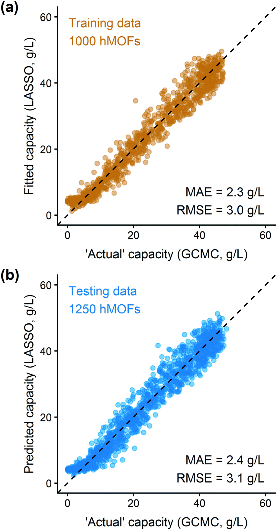 | ||
| Fig. 4 Parity plot for training and testing data from the hMOF database using the sparse regression model for the hydrogen deliverable capacity between 100 bar and 2 bar at 77 K. Each point represents one MOF structure from the hMOF database. (a) Training data is displayed in orange; (b) testing data is in blue. The data are tightly correlated with R2 = 0.96 for the training data and Q2 = 0.96 using cross-validation. | ||
Finally, we evaluated the cross-validated R2 value, also denoted Q2, which characterizes how much variance in the testing data is captured by the model. We calculated Q2 to assess the accuracy of predicting validation data outside of the model fit.69 The formula for calculating Q2 is analogous to the coefficient of determination R2:
 | (7) |
This equation is identical to R2 except for the method of predicting each yi. We calculated Q2 using K = 10-fold cross-validation, which randomly splits the data into ten sets, then iteratively fits a model using nine of them while making predictions on the remaining holdout partition. This procedure is marked with the y(i) notation above and ensures that the test data for predictions is distinct from the data used to fit the model. Since R2 is based on the training data, it will monotonically increase with overfitting, whereas Q2 will decrease once the model no longer generalizes to the testing data.70
Using the hMOF data, we obtain an extraordinary Q2 of 0.96, supporting our claims that the model identified properties of the energy histogram that are predictive to other MOFs. To establish a baseline value for Q2, we shuffled the explanatory and response variables (Fig. S28†), which feeds the model “junk” data for the variables without changing their statistical distributions.71 From this experiment, we find that the model has a baseline Q2 of 0, which is the same as a naive model based on the mean uptake without other parameters. Thus, the model is fitting important features of the data and not reporting spurious correlations based on noise.
3.2 Method generality
After training a LASSO regression model and testing its prediction accuracy for hydrogen storage, we explored the generality and limitations of the methodology. Most importantly, we wanted to test the transferability to other sets of MOFs and other simple adsorbate molecules. We also evaluated the method's robustness by modifying the parameters for histogram binning and model regularization. From these studies, we learn more about the model's usefulness for screening other systems. | ||
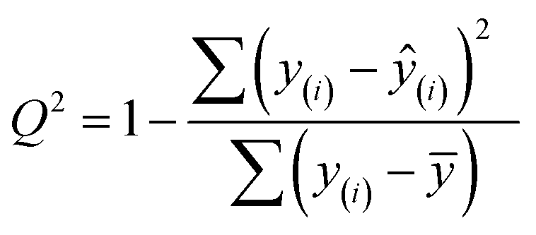
| Fig. 5 Application of the energy histogram model to other MOF databases. The property to be predicted is the deliverable hydrogen capacity between 100 bar and 2 bar at 77 K. Parity plots of (a) ToBaCCo test data using a model trained using ToBaCCo MOF data, (b) ToBaCCo testing data using the trained hMOF model, shaded by the largest cavity diameter (LCD) of each MOF. Note the poor performance for large pore MOFs, (c) predictions on ToBaCCo testing data using a model trained with 500 hMOFs and 500 ToBaCCo MOFs (“mixed model”), and (d) testing the mixed model on a random sample of CCDC MOFs. Many of the CCDC MOFs have low porosity, which the model successfully captures by predicting low gas uptake for these structures. | ||
Fig. 5(b) shows that the hMOF-trained model is also predictive of deliverable capacity in the ToBaCCo MOFs without retraining, except for large pore MOFs where the model overpredicts. Comparing the geometric properties of the hMOF and ToBaCCo databases (Fig. S19†), we see that there are many ToBaCCo MOFs with a largest cavity diameter larger than any MOF in the hMOFs, so the hMOF-trained model does not adequately characterize these MOFs. Bobbitt et al. previously demonstrated that if a pore is too large, the H2–MOF interactions are too weak to sufficiently bind hydrogen, so this region is wasted space in the MOF and thus in the vehicle fuel tank.35 Overall, the issue in transferability highlights that extrapolation should be used with caution. In this instance, the training set did not have a sufficiently diverse set of pore characteristics, which could have yielded misleading results if the model validation had been skipped.
To account for the differences in pore characteristics between the two databases, we trained a “mixed model” using a training set of 500 hMOFs and 500 ToBaCCo MOFs randomly selected from their parent databases. Fig. S24† confirms that the coefficient for weak H2–MOF interactions is smaller in the combined model, which corrects the earlier overprediction in large pore MOFs. Applying the mixed model, we see that the predictions on other ToBaCCo MOFs are considerably better than the hMOF-trained model (Fig. 5(c)). Furthermore, we verified that the mixed model generalizes to several topologies and pore shapes (Fig. S27†). Since the model is only based on the energy histogram, it does not have any explicit dependence on spatial or textural properties. The simple one-dimensional descriptor derived from the energy landscape is all that is needed to predict hydrogen uptake in MOFs to within a reasonable error.
We also tested the applicability of the mixed model for screening experimentally-derived structures in the CCDC MOF database using a random subset of 1000 MOFs for validation.26 From the parity plot in Fig. 5(d), we find that the mixed regression model predicts the hydrogen deliverable capacity for the CCDC MOFs reasonably well. Model errors tend to be overpredictions, but this type of error is not a problem for purposes of screening for top materials. A false positive for a “top MOF” (which will result in an additional GCMC simulation of a poorly performing material) is preferable to a false negative (excluding a top candidate), since these simulations are not prohibitively expensive individually. We expect that our method could also be applied to other classes of nanoporous materials, such as zeolites, covalent organic frameworks, or zeolitic imidazolate frameworks, using suitable potentials and validation tests.
We trained a model using 1000 hMOFs to predict the deliverable capacity of methane at 298 K between 65 bar and 5.8 bar.31,73 From the parity plot in Fig. 6(a), we see that the model can accurately predict the deliverable capacity of methane in the hMOF testing data set. The model overpredicts the capacity in MOFs with very poor uptake, but these MOFs would not be interesting for gas storage applications. The accuracy for well-performing MOFs is more important for ranking and screening purposes. By analyzing the coefficients for the deliverable capacity model in Fig. 6(b), we observe similar adsorption design principles as for hydrogen. Somewhat weakly attractive regions of the MOF are ideal for gas storage and release, and strongly adsorbing sites will not release bound methane at the delivery conditions. The predicted optimal heat of adsorption for methane is larger in magnitude than that for hydrogen, which agrees with physical intuition about these two molecules. Our model predicts the optimal energy range for methane is between 6–12 kJ mol−1, which is mostly in agreement with results (10.5–14.5 kJ mol−1) reported by Gómez-Gualdrón et al. based on high-throughput GCMC simulations.74
 | ||
| Fig. 6 The energy histogram regression approach can be adapted to methane. (a) Parity plot of hMOF database testing data. (b) Regression coefficients for the deliverable capacity of methane at room temperature between 65 and 5.8 bar. | ||
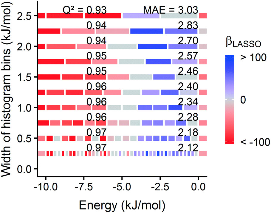 | ||
| Fig. 7 Model coefficients are robust to histogram binning strategy. Different bin widths were tested in 0.25 kJ mol−1 increments, designated by the position of the model along the y axis. We used a width of 1.0 kJ mol−1 for hydrogen adsorption models discussed elsewhere in the paper. The energy range for each bin is shown by bars spanning along the x axis and colored by the β of the corresponding LASSO model trained on 1000 hMOFs. | ||
In selecting a statistical learning model, we decided to use LASSO for its simplicity, interpretability, and resistance to overfitting. However, there are other regularization methods for fitting regression models, so we tested two other approaches for fitting. Ridge regression75 is conceptually similar to LASSO, except the penalty term is based on the L2-norm of the coefficients (the penalty term λ∑|βj| becomes λ∑(βj)2). One consequence is that ridge regression cannot shrink coefficients to zero. We also examined the ordinary least squares approach to multiple linear regression (MLR), which does not include regularization, as a base case. From Fig. S21,† we find that all three of these models yield consistent predictive performance. Regularization is not essential to obtain accurate predictions using our approach, but LASSO has the potential to simplify the model.
We also tested the model's sensitivity to the number of MOFs used in the training set. Calculating hydrogen adsorption in 1000 MOFs at two pressures is highly feasible. However, for some adsorbates (e.g. water), the simulations are particularly challenging, and even 500 calculations may be prohibitively expensive. For hydrogen, we determined that the model was well-converged when using 1000 MOFs for training, but as few as 150 training samples may still give reasonably similar results (Table S9†).
3.3 Accelerating MOF screening
As a demonstration of our method, we screened the CCDC MOF database to find top candidates for hydrogen storage. Specifically, we focused on the volumetric deliverable capacity, because it directly influences the fuel tank size for vehicular applications.36,76,77 Based on the parity plot in Fig. 5(d), a LASSO regression model is suitable for quantitatively predicting the deliverable capacity of hydrogen for materials selection. Instead of a brute force GCMC screening on the full database, which is computationally expensive, our screening workflow consisted of calculating the energy histogram for each material, running the sparse regression model to predict the deliverable capacity, and selecting the top candidates to validate using standard GCMC simulations.As reported in the literature, the majority of structures in the CCDC MOF subset are nonporous.26 It is common to add a textural analysis step to screening workflows in order to avoid simulations on nonporous materials, but this step is not necessary in our energy histogram analysis. Our model automatically assigns a low uptake to nonporous materials, which have a large repulsive bin in the energy histogram calculation. A more complex textural analyses is not required and would not reduce the overall simulation time much, because the energy-based approach is sufficiently rapid.
776 structures in the CCDC MOF subset and flag the top 1000 structures. Then, we ran GCMC simulations on the top 1000 to verify the accuracy of the model and to determine which materials would be most interesting for further consideration. We found suitable agreement between the regression predictions and GCMC results (Fig. S29†), providing additional confidence in the machine learning accelerated workflow.
In visualizing the top candidates flagged by the regression model, we observed that some of the structures were not MOFs. Some of the structures only included an unrealistic arrangement of metallic atoms in a unit cell, without any organic motifs. These structural errors can be attributed to the difficulty of automated structure curation and may be a consequence of enabling a flag in the solvent removal script to remove all monodentate solvents. We performed structural analyses using Zeo++78 to determine the dimensionality of connected framework atoms. Overall, 26.5% of the desolvated MOFs in the CCDC subset were classified as 3D frameworks. Among the top 1000 structures, 119 contained a 3D framework, and 51 of these had a hydrogen deliverable capacity above 45 g L−1 as calculated by GCMC.
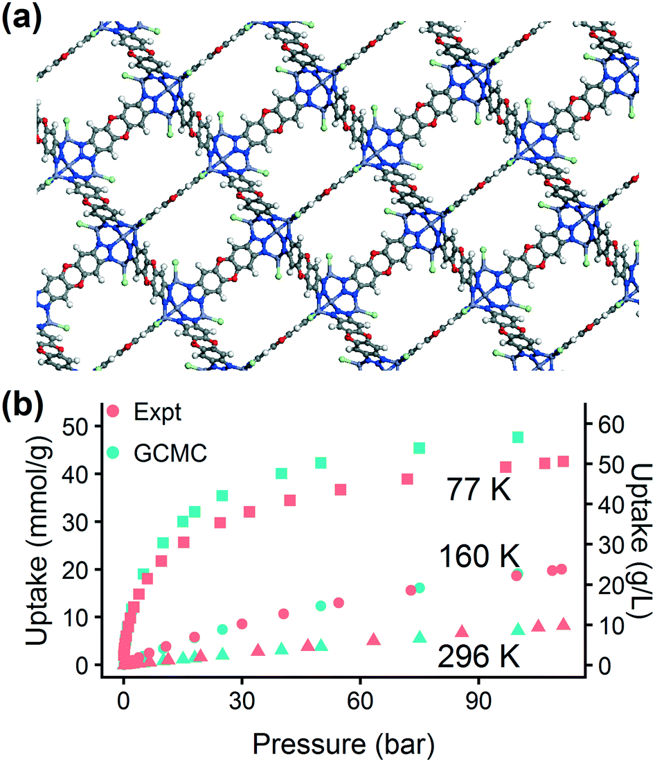 | ||
| Fig. 8 Applying the trained hMOF model for screening the CCDC MOF database. (a) Structure and (b) hydrogen adsorption isotherm for MFU-4l, a high-performing MOF selected for experimental validation. Red symbols are isotherm points from experiment and blue points are from GCMC simulations at 77 K (squares), 160 K (circles), and 296 K (triangles). | ||
The chosen MOF, MFU-4l, can be synthesized using several different metals. Using the machine learning approach, in less than an hour we obtained a preliminary answer to the question: will changing the metal composition have a significant effect on the MOF's hydrogen storage properties? We tested this effect computationally by replacing the metal atoms in the MFU-4l crystal structure with four candidates (Co, Mn, Ni, and Zn). We calculated the energy histograms for each material and predicted the uptake using the LASSO model, finding no significant difference in gas uptake between the structures, which we confirmed with GCMC simulations. Thus, we proceeded with experimental synthesis and characterization of MFU-4l(Zn) due to the ease of synthesis using Zn.
The excellent agreement between calculated and experimental N2 isotherms (Fig. S4–S6†) suggests that a highly crystalline and well-activated MFU-4l was achieved. It is crucial to check and confirm the quality of the synthesized MOF since the calculations were performed on ideal structures with no defects or solvent molecules in the structure. After confirming the quality of the MFU-4l sample, we measured the high pressure H2 isotherms (Fig. 8) using the guest-free MFU-4l crystals, which showed 36 g L−1 deliverable H2 uptake at isothermal conditions of 77 K using 100 bar for storage and 2 bar for delivery. The agreement between the calculated and experimental high pressure H2 isotherms confirms the validity of our approach.§ We also note that alternative delivery conditions of 5 bar, 160 K have been more recently proposed to extract additional storage capacity from nanoporous materials,79 and studies have begun testing these operating parameters for MOF design.36,76 We measured a hydrogen deliverable capacity of 47 g L−1 for storage at 100 bar, 77 K and delivery at 5 bar, 160 K and 29 g L−1 for delivery at 5 bar, 77 K. These properties place MFU-4l among the top-performing MOFs for hydrogen storage among a diverse series of MOFs that were recently benchmarked experimentally and computationally.77
953 hMOFs for hydrogen storage required approximately 500000 CPU hours of compute time.35 In contrast, the machine learning workflow in this work only required 97 CPU hours to calculate the energy grids for the same hMOF database, another 13 hours to bin these grids into energy histograms, and less than 15 minutes to fit and run the regression analyses. Although the machine learning workflow requires training and validation data from GCMC simulations (or experiment), it is also more scalable to large MOF databases. Once the approach has been validated for reliability, additional structures are computationally inexpensive to test, requiring seconds per MOF instead of hours or days. On the other hand, the number of GCMC simulations required in a conventional brute force screening approach scales linearly with the number of structures. For example, screening another 130000 hMOFs would require another 500000 CPU hours using the brute force approach. Using the new approach, the same task could be completed using 100 hours upfront to flag the most promising structures, then targeting GCMC calculations on the number of desired candidates. The time savings from this method may be even greater in systems where GCMC simulations are difficult.
4 Conclusions
In this work, we demonstrated that sorbate–sorbent energy histograms are an effective descriptor to predict gas adsorption in MOFs, enabling rapid screening of large numbers of MOFs. At its core, the method correlates gas uptake with information about MOF–guest interactions, which is ultimately the property that governs physisorption in GCMC simulations and experiment. This physical basis makes the approach accurate, transferable, and robust. The approach can also provide data-driven insights about ideal materials for a given application. We applied a trained model to screen 54776 structures in the CCDC MOF subset and identify the top candidates with less than 10% of the total computational resources of a brute force screening, even when accounting for validation simulations. We synthesized one of these MOFs, MFU-4l(Zn) and confirmed its high hydrogen storage capacity experimentally. The approach presented in this work is a promising method to accelerate MOF screening and to reveal key material properties for a given application, which may then guide material design. Future work will focus on testing the range of applicability of the method.
Conflicts of interest
The authors declare the following competing financial interest(s): O. K. F. and R. Q. S. have a financial interest in NuMat Technologies, a startup company that is seeking to commercialize MOFs.Acknowledgements
This research was supported by the U.S. Department of Energy, Office of Basic Energy Sciences, Division of Chemical Sciences, Geosciences and Biosciences under Award No. DE-FG02-17ER16362. B. J. B. also acknowledges a research grant through the Data Science Initiative at Northwestern University and a National Science Foundation Graduate Research Fellowship under Grant No. DGE-1324585. This research was supported in part through the computational resources and staff contributions provided for the Quest high-performance computing facility at Northwestern University, which is jointly supported by the Office of the Provost, the Office for Research, and Northwestern University Information Technology.References
- Honda Clarity, https://automobiles.honda.com/clarity-fuel-cell, (accessed 2017-12-01) Search PubMed.
- Toyota Mirai, https://ssl.toyota.com/mirai/fcv.html, (accessed 2017-12-01) Search PubMed.
- Hyundai Tucson Fuel Cell, https://www.hyundaiusa.com/tucsonfuelcell/index.aspx, (accessed 2017-12-01) Search PubMed.
- General Motors Fuel Cell, http://www.gm.com/mol/m-2017-oct-1006-fuel-cell-platform.html, (accessed 2017-12-01) Search PubMed.
- US Fuel Cell Car Sales, http://carsalesbase.com/us-car-sales-data/toyota/toyota-mirai/, (accessed 2017-12-01) Search PubMed.
- Alstom Coradia iLint Train, http://www.alstom.com/products-services/product-catalogue/rail-systems/trains/products/coradia-ilint-regional-train/, (accessed 2017-12-01) Search PubMed.
- Cold/Cryogenic Composites for Hydrogen Storage Applications in FCEVs, https://energy.gov/sites/prod/files/2015/11/f27/fcto_cold_cryo_h2_storage_wkshp_1_doe.pdf, (accessed 2017-02-08) Search PubMed.
- DOE Hydrogen Storage Targets, https://energy.gov/eere/fuelcells/downloads/doe-targets-onboard-hydrogen-storage-systems-light-duty-vehicles, (accessed 2017-12-01) Search PubMed.
- W. Zhou, H. Wu, M. R. Hartman and T. Yildirim, J. Phys. Chem. C, 2007, 111, 16131–16137 CrossRef CAS.
- B. Panella and M. Hirscher, Adv. Mater., 2005, 17, 538–541 CrossRef CAS.
- M. P. Suh, H. J. Park, T. K. Prasad and D.-W. Lim, Chem. Rev., 2011, 112, 782–835 CrossRef PubMed.
- J. Sculley, D. Yuan and H.-C. Zhou, Energy Environ. Sci., 2011, 4, 2721–2735 RSC.
- P. Jena, J. Phys. Chem. Lett., 2011, 2, 206–211 CrossRef CAS.
- Y. Sun, L. Wang, W. A. Amer, H. Yu, J. Ji, L. Huang, J. Shan and R. Tong, J. Inorg. Organomet. Polym., 2013, 23, 270–285 CrossRef CAS.
- H. W. Langmi, J. Ren, B. North, M. Mathe and D. Bessarabov, Electrochim. Acta, 2014, 128, 368–392 CrossRef CAS.
- Y. Basdogan and S. Keskin, CrystEngComm, 2015, 17, 261–275 RSC.
- S. Niaz, T. Manzoor and A. H. Pandith, Renewable Sustainable Energy Rev., 2015, 50, 457–469 CrossRef CAS.
- S. Kitagawa and H.-C. Zhou, Chem. Soc. Rev., 2014, 43, 5415–5418 RSC.
- H.-C. Zhou, J. R. Long and O. M. Yaghi, Chem. Rev., 2012, 112, 673–674 CrossRef CAS PubMed.
- J.-R. Li, R. J. Kuppler and H.-C. Zhou, Chem. Soc. Rev., 2009, 38, 1477–1504 RSC.
- H. Furukawa, K. E. Cordova, M. O'Keeffe and O. M. Yaghi, Science, 2013, 341, 1230444 CrossRef PubMed.
- S. M. Cohen, Chem. Rev., 2012, 112, 970–1000 CrossRef CAS PubMed.
- O. M. Yaghi, M. O'Keeffe, N. W. Ockwig, H. K. Chae, M. Eddaoudi and J. Kim, Nature, 2003, 423, 705–714 CrossRef CAS PubMed.
- T. Islamoglu, S. Goswami, Z. Li, A. J. Howarth, O. K. Farha and J. T. Hupp, Acc. Chem. Res., 2017, 50, 805–813 CrossRef CAS PubMed.
- Y. G. Chung, J. Camp, M. Haranczyk, B. J. Sikora, W. Bury, V. Krungleviciute, T. Yildirim, O. K. Farha, D. S. Sholl and R. Q. Snurr, Chem. Mater., 2014, 26, 6185–6192 CrossRef CAS.
- P. Z. Moghadam, A. Li, S. B. Wiggin, A. Tao, A. G. P. Maloney, P. A. Wood, S. C. Ward and D. Fairen-Jimenez, Chem. Mater., 2017, 29, 2618–2625 CrossRef CAS.
- C. E. Wilmer, M. Leaf, C. Y. Lee, O. K. Farha, B. G. Hauser, J. T. Hupp and R. Q. Snurr, Nat. Chem., 2012, 4, 83–89 CrossRef CAS PubMed.
- M. Fernandez, P. G. Boyd, T. D. Daff, M. Z. Aghaji and T. K. Woo, J. Phys. Chem. Lett., 2014, 5, 3056–3060 CrossRef CAS PubMed.
- Y. J. Colón, D. A. Gómez-Gualdrón and R. Q. Snurr, Cryst. Growth Des., 2017, 17, 5801–5810 CrossRef.
- R. L. Martin, C. M. Simon, B. Smit and M. Haranczyk, J. Am. Chem. Soc., 2014, 136, 5006–5022 CrossRef CAS PubMed.
- C. M. Simon, J. Kim, D. A. Gomez-Gualdron, J. S. Camp, Y. G. Chung, R. L. Martin, R. Mercado, M. W. Deem, D. Gunter, M. Haranczyk, D. S. Sholl, R. Q. Snurr and B. Smit, Energy Environ. Sci., 2015, 8, 1190–1199 RSC.
- C. M. Simon, J. Kim, L.-C. Lin, R. L. Martin, M. Haranczyk and B. Smit, Phys. Chem. Chem. Phys., 2014, 16, 5499–5513 RSC.
- A. W. Thornton, C. M. Simon, J. Kim, O. Kwon, K. S. Deeg, K. Konstas, S. J. Pas, M. R. Hill, D. A. Winkler, M. Haranczyk and B. Smit, Chem. Mater., 2017, 29, 2844–2854 CrossRef CAS PubMed.
- Y. J. Colón, D. Fairen-Jimenez, C. E. Wilmer and R. Q. Snurr, J. Phys. Chem. C, 2014, 118, 5383–5389 CrossRef.
- N. S. Bobbitt, J. Chen and R. Q. Snurr, J. Phys. Chem. C, 2016, 120, 27328–27341 CrossRef CAS.
- D. A. Gómez-Gualdrón, Y. J. Colón, X. Zhang, T. C. Wang, Y.-S. Chen, J. T. Hupp, T. Yildirim, O. K. Farha, J. Zhang and R. Q. Snurr, Energy Environ. Sci., 2016, 9, 3279–3289 RSC.
- S. Han, Y. Huang, T. Watanabe, Y. Dai, K. S. Walton, S. Nair, D. S. Sholl and J. C. Meredith, ACS Comb. Sci., 2012, 14, 263–267 CrossRef CAS PubMed.
- Y. G. Chung, D. A. Gómez-Gualdrón, P. Li, K. T. Leperi, P. Deria, H. Zhang, N. A. Vermeulen, J. F. Stoddart, F. You, J. T. Hupp, O. K. Farha and R. Q. Snurr, Sci. Adv., 2016, 2, e1600909 CrossRef PubMed.
- C. M. Simon, R. Mercado, S. K. Schnell, B. Smit and M. Haranczyk, Chem. Mater., 2015, 27, 4459–4475 CrossRef CAS.
- S. Curtarolo, G. L. Hart, M. B. Nardelli, N. Mingo, S. Sanvito and O. Levy, Nat. Mater., 2013, 12, 191–201 CrossRef CAS PubMed.
- P. Canepa, C. A. Arter, E. M. Conwill, D. H. Johnson, B. A. Shoemaker, K. Z. Soliman and T. Thonhauser, J. Mater. Chem. A, 2013, 1, 13597–13604 RSC.
- P. Wollmann, M. Leistner, U. Stoeck, R. Grünker, K. Gedrich, N. Klein, O. Throl, W. Grählert, I. Senkovska, F. Dreisbach and S. Kaskel, Chem. Commun., 2011, 47, 5151–5153 RSC.
- J. A. Gee, K. Zhang, S. Bhattacharyya, J. Bentley, M. Rungta, J. S. Abichandani, D. S. Sholl and S. Nair, J. Phys. Chem. C, 2016, 120, 12075–12082 CrossRef CAS.
- H. Demir, K. S. Walton and D. S. Sholl, J. Phys. Chem. C, 2017, 121, 20396–20406 CrossRef CAS.
- B. Panella, M. Hirscher and S. Roth, Carbon, 2005, 43, 2209–2214 CrossRef CAS.
- J. Goldsmith, A. G. Wong-Foy, M. J. Cafarella and D. J. Siegel, Chem. Mater., 2013, 25, 3373–3382 CrossRef CAS.
- A. Ahmed, Y. Liu, J. Purewal, L. D. Tran, A. G. Wong-Foy, M. Veenstra, A. J. Matzger and D. J. Siegel, Energy Environ. Sci., 2017, 10, 2459–2471 RSC.
- C. E. Wilmer, O. K. Farha, Y.-S. Bae, J. T. Hupp and R. Q. Snurr, Energy Environ. Sci., 2012, 5, 9849–9856 RSC.
- M. Fernandez and A. S. Barnard, ACS Comb. Sci., 2016, 18, 243–252 CrossRef CAS PubMed.
- M. Fernandez, T. K. Woo, C. E. Wilmer and R. Q. Snurr, J. Phys. Chem. C, 2013, 117, 7681–7689 CrossRef CAS.
- E. Braun, A. F. Zurhelle, W. Thijssen, S. K. Schnell, L.-C. Lin, J. Kim, J. A. Thompson and B. Smit, Mol. Syst. Des. Eng., 2016, 1, 175–188 RSC.
- Y. J. Colón and R. Q. Snurr, Chem. Soc. Rev., 2014, 43, 5735–5749 RSC.
- M. Pardakhti, E. Moharreri, D. Wanik, S. L. Suib and R. Srivastava, ACS Comb. Sci., 2017, 19, 640–645 CrossRef CAS PubMed.
- M. Fernandez, N. R. Trefiak and T. K. Woo, J. Phys. Chem. C, 2013, 117, 14095–14105 CrossRef CAS.
- D. Paik, M. Haranczyk and J. Kim, J. Mol. Graphics Modell., 2016, 66, 91–98 CrossRef CAS PubMed.
- D. Ongari, P. G. Boyd, S. Barthel, M. Witman, M. Haranczyk and B. Smit, Langmuir, 2017, 33, 14529–14538 CrossRef CAS PubMed.
- D. Dubbeldam, S. Calero, D. E. Ellis and R. Q. Snurr, Mol. Simul., 2016, 42, 81–101 CrossRef CAS.
- A. K. Rappe, C. J. Casewit, K. S. Colwell, W. A. Goddard and W. M. Skiff, J. Am. Chem. Soc., 1992, 114, 10024–10035 CrossRef CAS.
- A. Michels, W. de Graaff and C. A. Ten Seldam, Physica, 1960, 26, 393–408 CrossRef CAS.
- F. Darkrim and D. Levesque, J. Chem. Phys., 1998, 109, 4981–4984 CrossRef CAS.
- J. Liu, J. T. Culp, S. Natesakhawat, B. C. Bockrath, B. Zande, S. G. Sankar, G. Garberoglio and J. K. Johnson, J. Phys. Chem. C, 2007, 111, 9305–9313 CrossRef CAS.
- M. G. Martin and J. I. Siepmann, J. Phys. Chem. B, 1998, 102, 2569–2577 CrossRef CAS.
- Materials Studio, Accelrys Software Inc., San Diego, CA 92121, USA, 2001 Search PubMed.
- R. Tibshirani, J. R. Stat. Soc. Series B Stat. Methodol., 1996, 58, 267–288 Search PubMed.
- R Core Team, R: A Language and Environment for Statistical Computing, R Foundation for Statistical Computing, Vienna, Austria, 2017 Search PubMed.
- J. Friedman, T. Hastie and R. Tibshirani, J. Stat. Softw., 2010, 33, 1–22 Search PubMed.
- D. Denysenko, M. Grzywa, M. Tonigold, B. Streppel, I. Krkljus, M. Hirscher, E. Mugnaioli, U. Kolb, J. Hanss and D. Volkmer, Chem. – Eur. J., 2011, 17, 1837–1848 CrossRef CAS PubMed.
- Y. Peng, V. Krungleviciute, I. Eryazici, J. T. Hupp, O. K. Farha and T. Yildirim, J. Am. Chem. Soc., 2013, 135, 11887–11894 CrossRef CAS PubMed.
- G. Schüürmann, R.-U. Ebert, J. Chen, B. Wang and R. Kühne, J. Chem. Inf. Model., 2008, 48, 2140–2145 CrossRef PubMed.
- J. A. Colton and K. M. Bower, Int. Soc. Six Sigma Prof. EXTRAOrdinary Sense, 2002, vol. 3, pp. 20–22 Search PubMed.
- C. Rücker, G. Rücker and M. Meringer, J. Chem. Inf. Model., 2007, 47, 2345–2357 CrossRef PubMed.
- B. J. Sikora, R. Winnegar, D. M. Proserpio and R. Q. Snurr, Microporous Mesoporous Mater., 2014, 186, 207–213 CrossRef CAS.
- ARPA-E Methane Opportunities for Vehicular Energy (MOVE), 2012 Search PubMed.
- D. A. Gómez-Gualdrón, C. E. Wilmer, O. K. Farha, J. T. Hupp and R. Q. Snurr, J. Phys. Chem. C, 2014, 118, 6941–6951 CrossRef.
- A. E. Hoerl and R. W. Kennard, Technometrics, 1970, 12, 55–67 CrossRef.
- D. A. Gómez-Gualdrón, T. C. Wang, P. García-Holley, R. M. Sawelewa, E. Argueta, R. Q. Snurr, J. T. Hupp, T. Yildirim and O. K. Farha, ACS Appl. Mater. Interfaces, 2017, 9, 33419–33428 CrossRef PubMed.
- P. García-Holley, B. Schweitzer, T. Islamoglu, Y. Liu, L. Lin, S. Rodriguez, M. H. Weston, J. T. Hupp, D. A. Gómez-Gualdrón, T. Yildirim and O. K. Farha, ACS Energy Lett., 2018, 3, 748–754 CrossRef.
- T. F. Willems, C. H. Rycroft, M. Kazi, J. C. Meza and M. Haranczyk, Microporous Mesoporous Mater., 2012, 149, 134–141 CrossRef CAS.
- D. Siegel, B. Hardy and HSECoE Team, Engineering an Adsorbent-Based Hydrogen Storage System: What Have We Learned?, https://www.energy.gov/sites/prod/files/2015/02/f19/fcto_h2_storage_summit_siegel.pdf, 2015, (accessed 2018-03-23) Search PubMed.
Footnotes |
| † Electronic supplementary information (ESI) available: Coefficients of the trained regression models, top MOF candidates, experimental characterization, simulation force field parameters, and other statistical analyses. See DOI: 10.1039/c8me00050f |
| ‡ Since the Feynman–Hibbs correction term in the potential contains temperature, we recalculated the energy grids and histograms at 160 K for the higher temperature results. See Fig. S13.† |
| § Our H2 uptake measurements are also in agreement with the original experimental study67 for MFU-4l, which reported H2 uptake measurements up to 20 bar. |
| This journal is © The Royal Society of Chemistry 2019 |