Kinetic energy densities based on the fourth order gradient expansion: performance in different classes of materials and improvement via machine learning
Pavlo
Golub
 * and
Sergei
Manzhos
*
Department of Mechanical Engineering, National University of Singapore, Block EA #07-08, 9 Engineering Drive 1, Singapore 117576. E-mail: pavelgolub87@gmail.com; mpemanzh@nus.edu.sg; Fax: +65 6779 1459; Tel: +65 6516 4605
First published on 29th November 2018
Abstract
We study the performance of fourth-order gradient expansions of the kinetic energy density (KED) in semi-local kinetic energy functionals depending on the density-dependent variables. The formal fourth-order expansion is convergent for periodic systems and small molecules but does not improve over the second-order expansion (the Thomas–Fermi term plus one-ninth of the von Weizsäcker term). Linear fitting of the expansion coefficients somewhat improves on the formal expansion. The tuning of the fourth order expansion coefficients allows for better reproducibility of the Kohn–Sham kinetic energy density than the tuning of the second-order expansion coefficients alone. The possibility of a much more accurate match with the Kohn–Sham kinetic energy density by using neural networks (NN) trained using the terms of the 4th order expansion as density-dependent variables is demonstrated. We obtain ultra-low fitting errors without overfitting of NN parameters. Small single hidden layer neural networks can provide good accuracy in separate KED fits of each compound, while for joint fitting of KEDs of multiple compounds multiple hidden layers were required to achieve good fit quality. The critical issue of data distribution is highlighted. We also show the critical role of pseudopotentials in the performance of the expansion, where in the case of a too rapid decay of the valence density at the nucleus with some pseudopotentials, numeric instabilities can arise.
Introduction
The search for the orbital-free form of the non-interacting kinetic energy functional (KEF), or more narrowly the kinetic energy density functional (KEDF), remains one of the most challenging tasks in density-functional theory (DFT).1,2 Finding such an expression would be an enormous boon for computational materials science, since in that case instead of solving self-consistently for a set of single-electron wavefunctions using the Kohn–Sham (KS) equation,3 one would need to solve self-consistently only the minimization problem of the total energy of the system E[n(r)] with respect to the electron density n(r), | (1) |
Here μ is the chemical potential that aims to ensure the normalization condition  , where Nel is the number of electrons, and Vext(r) is an external field, if present (for simplicity, we will ignore spin). Indeed, while other components in DFT partitioning of the total energy – the Hartree energy, nuclear–electron interaction energy, and exchange–correlation energy – can be explicitly represented via the electron density with satisfactory accuracy, good approximations to the kinetic energy (KE)
  or kinetic energy density (KED) τ[n(r)] as a functional of only density-dependent quantities are still missing (note that subsequently we consider τ[n(r)] = τ(r) as an explicit function of r in this work). They are the main subject of developments in orbital-free DFT (OF-DFT).4 Existing approximations to the kinetic energy functionals (KEF) work well, i.e. provide accuracy similar to KS-DFT, only when the density is slowly varying, specifically, for light metals5–10 and some simplest semiconductors,11 but there is still no KEF that would be sufficiently accurate for molecular densities to allow for molecular structure optimization with accuracy approaching that of Kohn–Sham DFT in applications.
One of the earliest and most straightforward methods for representing the KE is an expansion in different orders of the gradient of the electron density. Initially introduced by Kirzhnits12 as a quantum correction to the Thomas–Fermi model for atoms,13,14 this method naturally takes the Thomas–Fermi functional as the zero-order term
 | (2) |
 | (3) |
Further developments of the gradient expansion method by Hodges16 and Murphy17 introduced fourth-order and sixth-order corrections respectively (the dependence of the electron density on r in eqn (4) and (5) is omitted for brevity):
 | (4) |
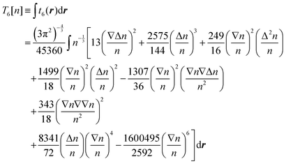 | (5) |
Here we use capital with subscript Ti to define terms of order i in the gradient expansion of kinetic energy (below, we occasionally omit the dependence of the kinetic energy and its terms on the electron density for brevity), and small ti(r) to define the corresponding terms in the space-dependent kinetic energy density τ[n(r)]. In turn, the whole gradient expansion of order k is defined with the corresponding superscript, i.e. , and
, and  .
.
These corrections had some success. For example, it was shown that the fourth-order gradient expansion T(4) = T0 + T2 + T4 gives the atomic Hartree–Fock kinetic energy with an error of less than 1% based on Hartree–Fock electron densities,18,19 which were calculated from analytic Hartree–Fock atomic wave functions by Clementi and Roetti.20 Although the performance of T(4) for molecules, calculated with a Gaussian basis, was not so impressive and resulted in errors which were more than two times larger than the errors from the second-order expansion T(2),21 it was shown that the use of a modified expansion with a scaled fourth-order term9T(4)m = T0 + T2 + λT4 improves the accuracy and can make the error less than 1%.21–23 Apparently, pseudopotentials were not used in those tests, meaning that the results were affected by the strongly corrugated (rapidly changing) core densities. It is worth noting that the use of the projector wave-augmented method (PAW)24 offers an alternative to the pseudopotential way of treating core electron states in the context of orbital-free density functional calculations,25 however this direction of research is not as often used in applications to OF-DFT as the pseudopotential approach.
Numeric convergence issues associated with higher order derivatives and their powers complicate the use of high-order gradient expansion terms. The gradient expansion terms of higher than the second order can diverge at long range.26 For example, it was suggested that such behavior makes T(4) unreliable for the description of electron gas models,27 does not allow for accurate reproduction of non-interacting kinetic energy contribution to the binding energies of molecules,28 and severely affects the self-consistent minimization procedure of eqn (1).26 Attempts to find an approximation that would circumvent this issue have had a degree of success in specific cases.29,30
The problems with convergence and accuracy are most apparent for calculations of atoms and molecules with an all-electron basis, but they might be not as severe when using pseudopotentials or/and in the case of solid-state periodic calculations, where large low-density regions typical for non-periodic systems are absent, and only the valence density is considered.31,32 Moreover, it was pointed out that this divergent behavior is global in the sense that each term is an integral over the entire electron distribution, while the respective kinetic energy density is in general finite except at specific points in space, which can be dealt with separately.27 Indeed, the consideration of 4th order terms, which were however adapted to satisfy scaling relations, exact conditions or slowly and rapidly varying density limits, has already been shown to substantially improve performance, and the modification of the corresponding functionals is the topic of much research.33–37
Overall, one may expect that T(4) can serve as a basis for a more reliable approximation, which nevertheless requires a tuning procedure to find an appropriate set of coefficients for the terms. Further, the sixth order expansion, eqn (5), was never thoroughly tested either for molecules or for solids. The improvements that could be achieved using T(6) with tuned coefficients are also worth considering but are not the subject of the present work.
The aim of the present work is to explore the extent of the use of the fourth-order gradient expansions, as published, with tuned coefficients, and when using the terms of the expansion as density dependent variables in a non-linear fit. We consider both solid-state systems and molecules. Specifically, we chose bulk light metals Li, Mg, and Al, which have sufficiently smooth valence densities such that (i) decent performance is expected and (ii) the availability of local pseudopotentials for these elements allows comparative tests in an existing code (PROFESS); we also chose bulk silicon as an example of a covalent system for which OF-DFT is currently still problematic with the best non-local functionals providing moderate accuracy.11,38 Finally, we chose small molecules, which are still off-limits to applied OF-DFT modeling. That is, we analyze several systems, which are progressively harder for OF-DFT approximations. We do so in the context of pseudopotential (PP) based calculations, which dominate materials modeling, otherwise the rapidly changing core electron density is expected to limit severely the performance of any KEF approximation. The resulting tuned KED expansions are tested on their ability to reproduce kinetic energy densities.
Albeit the condition of positivity of the Pauli potential and other properties of kinetic energy density39,40 can be enforced with the aim to improve non-empirical semi-local functionals,34,39–42 we do not impose them in our investigation. As has been demonstrated by Levy and Ou-Yang,39 the condition of positivity of the Pauli term is naturally satisfied with the decomposition of the KEDF solely into the Thomas–Fermi and full von Weizsäcker terms, but it holds no longer for the decompositions using higher order terms or using a scaled amount of the von Weizsäcker term. Also, imposing the coordinate scaling condition does not necessarily improve a machine learned KEDF, as has recently been shown for the simplest real system – the H2 molecule.43 The 4th order gradient expansion holds “as is” and we use its terms without further scaling of the respective derivative terms.
We use a machine learning (ML) approach, specifically neural networks (NN).44 ML has recommended itself as a useful approach for atomic and molecular simulations by providing extremely accurate fits of a number of parameters to reference data.45–48 In the field of OF-DFT, ML has already become an actively used tool, e.g. for approximation of the KED in one dimension as a function of the electron density by means of kernel ridge regression,49–51 the approximation for a non-local correction to the KE by means of convolutional neural networks,52 direct learning of the potential,53 and the attempt to construct a semi-local KEDF based on up to third-order gradients of the electron density with multi-layer NNs,54 to name but a few recent studies. Specifically, the NN approach has the advantage over some other ML techniques44 in that it is relatively easy to apply to the large data sets (millions of data) used in this work.
At first, we will concentrate on training of NNs for each compound separately to underline some important features concerning pseudopotentials and technical aspects of data distribution and provide reference accuracies. We then explore NN learning simultaneously of the KEDs of multiple components, which is necessary to arrive at a transferable KED functional.
Methods
DFT calculations were performed in Abinit 7.10.555,56 using the Perdew–Burke–Ernzerhof (PBE) functional.57 Molecules were placed inside large simulation cells with periodic boundary conditions. For bulk compounds, the conventional standard unit cells were used. Fermi–Dirac smearing was used in the case of Al, Mg and Li, with a corresponding smearing of 0.01 Ha. The resulting lattice parameters together with other calculation details are listed in Table 1. The plane-wave cutoffs were chosen based on convergence tests. The used k-point sampling grids provided converged results. The force tolerance was set to 5 × 10⁻⁶ Hartree per Bohr. The energy tolerance for the self-consistent minimization procedure was set to 10−10 Hartree. Goedeker–Teter–Hutter (GTH) pseudopotentials59,60 were used for Al, Mg, and Li (the case of a large core for the former two), while for O, H, C, and Si, as well as for Mg and Li with small-core PPs, Fritz–Haber–Institute (FHI) pseudo-potentials61,62 were taken.| Compound | Optimized lattice constants, a.u. | Experimental lattice constants,58 a.u. | Energy cutoff, Ha | k-point sampling | Sampling resolution of real-space grid, a.u. | Number of test and fitting points |
|---|---|---|---|---|---|---|
| a 2 valence electrons. b 10 valence electrons. c 1 valence electron. d 3 valence electrons. | ||||||
| Aluminum | 7.542 | 7.652 | 16.0 | 8 × 8 × 8 | 0.0250 | 9.2 × 10⁶ |
| Magnesium | a = 6.080a | a = 6.065 | 20.0 | 8 × 8 × 4 | 0.0334 | 3.4 × 10⁶ |
| c = 9.872a | b = 9.847 | |||||
| a = 6.127b | ||||||
| c = 9.947b | ||||||
| Lithium | 6.463c | 6.633 | 16.0 | 8 × 8 × 8 | 0.0334 | 2.7 × 10⁶ |
| 6.686d | ||||||
| Silicon | 10.327 | 10.263 | 24.0 | 8 × 8 × 8 | 0.0251 | 9.4 × 10⁶ |
| H2O | 15.118 | — | 20.0 | Γ point | 0.0501 | 9.15 × 10⁶ |
| C6H6 | 18.897 | — | 20.0 | Γ point | 0.0665 | 7.6 × 10⁶ |
The fitting was performed in the Matlab Neural Network Toolbox.63 The vector of NN input coordinates z contained up to five elements; all of them were terms entering T(4):
 | (6) |
The fitting target was chosen to be the scalar Kohn–Sham kinetic energy density  , where
  . The term z2(r) that we use was corrected by a quarter of the Laplacian of the electron density in order to make its shape locally compatible with the chosen form of τKS(r). The densities, gradients of the densities, Laplacians of the densities, and the kinetic energy densities were built directly from the corresponding plane-wave coefficients and output on real-space grids in the .cube format.64 The sizes of the ‘boxes’ in the cube files were identical to the corresponding simulation cells. Sampling resolutions for each compound are given in Table 1. The values of kinetic energies and total charges, computed as integrated values over the simulation cells, were ensured to match the output values from Abinit.
The general expression for NN learned KEDs takes the form46
 | (7) |
 , and biases
  . We use a linear activation function for the output layer, σout(x) = x. KN is the number of neurons in each hidden layer. The parameter “order” in t(order)(r) takes a value of 2 when only functions z1(r) and z2(r) are in the input vector, and a value of 4 when all five functions from eqn (6) are in the input vector (therefore underlining the relevance of these input vectors to 2nd and 4th order formal expansions, respectively).
When a single-hidden layer NN with a linear neuron in the hidden layer is used (σ1(x) = x), NN training is reduced to linear regression  (linear fit of expansion coefficients w(1)i). Subsequently we refer to linearly fitted KEDs as “fitted”. Non-linear NN fitting is designated as t(order),NN(r) with Nneurons neurons, and the neuron activation function in this case is sigmoidal
  . For NN training, the values at the grid points were mapped to the interval [−1.0, 1.0].
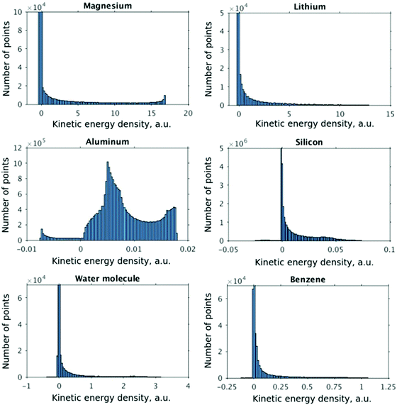
The distributions of the kinetic energy density values for the studied systems are shown in Fig. 1. The distributions are strongly non-uniform, which makes the data difficult to fit. Therefore, in order to ensure more appropriate coverage for each part of the distributions, the fit and test data were selected in the following way: four intervals were defined for scaled values of KED: [−1.0, −0.5], [−0.5, 0.0], [0.0, 0.5], and [0.5, 1.0]. The fraction of cube points drawn from each KED interval for use in fit and test sets was the higher the smaller the number of values in the corresponding part of the histogram of Fig. 1. If the number of data in a given interval was smaller than 1/5000th of the total number of points, all of them were drawn. This is a similar approach to histogram equalization.65 However, when systems with more complex than near-uniform (Li, Mg, and Al) electron density profiles are considered, even the above described approximate histogram equalization scheme is not sufficient. For example, in our investigation this was the case for Si, where numerical instabilities arose in the NN-fitted KED near the nucleus due to the relatively low number of sampling points, even though there was no parameter overfitting as the total number of data was overwhelmingly large compared to the number of NN parameters (see Fig. 1, silicon, the region with negative values of KED). Further equalization then was performed by producing additional cube files just around Si atoms with an approximately 2.5 times higher resolution. Thus, having in such a way two sets of cube files (one for the unit cell, another one for the near-atomic region), one half of test and fitting points was drawn from the first set, and the other half was drawn from the second set. NN fitting was done to minimize the root mean square error (RMSE) of the kinetic energy density
 | (8) |
At the start of the training procedure, the weights were initialized randomly with the Nguyen–Widrow initialization algorithm.66 The training was performed with the Levenberg–Marquardt algorithm,67,68 and stopped either when the minimum performance gradient became smaller than 10−10 or when the number of epochs exceeded 2000. The networks considered below showed no sign of overfitting during training i.e. the RMSE on the training set was of the same order as the RMSE on the test set.
OF-DFT calculations were carried out in PROFESS 3.069 using the PBE exchange–correlation functional with a plane wave cutoff of 3600 eV, which provided converged results.
Results
The performance of the formal gradient density expansion
The crystal structures of Li (bcc), Al (fcc), Mg (hcp), and Si (cubic diamond) as well as the molecular structures of H2O and C6H6 are shown in Fig. 2. The lines along which the representative plots of the kinetic energy density are computed with different approximations have the following directions: [100] for Al, [111] for Si, and along the line between atoms at (2/3, 1/3, 1/4) and (1/3, 2/3, 3/4) Wyckoff positions for Mg. For molecules, the lines are along interatomic bonds. The intervals over which the KED is plotted in Fig. 3–10 and 12–17 are shown as arrows in Fig. 2. We also examined 2D slices of the KED. The quality of the KED approximation with different 2nd and 4th order expansions is also shown in Fig. 3–10 on planes (passing through atoms) {1122} for Mg, {101} for Li, {101} for Al, and {111} for Si, as well as molecular planes.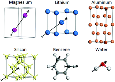 | ||
| Fig. 2 The crystal structures of Li, Al, Mg, and Si as well as the molecular structures of H2O and C6H6. The arrows indicate the directions and intervals along which the kinetic energy density is plotted in Fig. 3–10. Unit cells are shown for Li and Mg, and 2 unit cells for Al. | ||
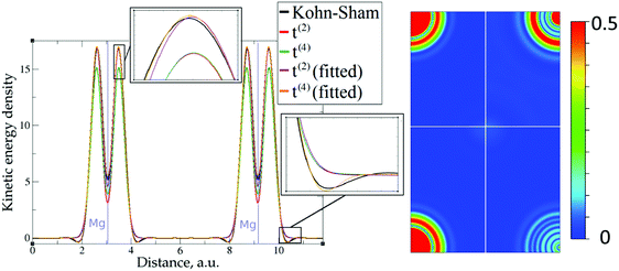 | ||
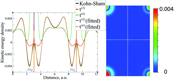
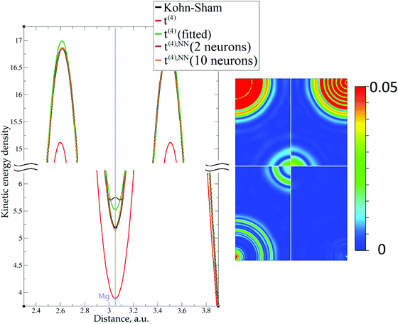
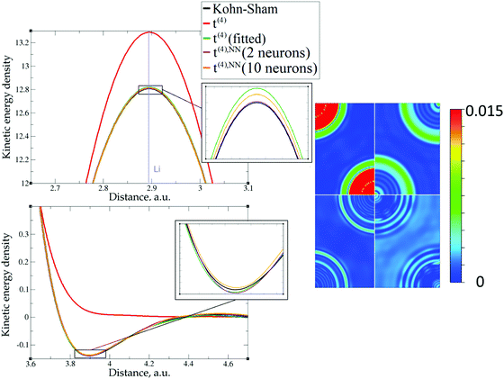
| Fig. 4 Kinetic energy density for magnesium (10 valence electrons), computed with Kohn–Sham DFT and with different gradient approximations for the KEDF (applied to the KS DFT density). On the left – the line along atoms at (2/3, 1/3, 1/4) and (1/3, 2/3, 3/4) Wyckoff positions; on the right – the projection of plane {1 1 2 2} with absolute differences between KEDs of different gradient approximations and the Kohn–Sham KED: upper left quadrant – formal t(2)(r), upper right quadrant – fitted t(2),fit(r), bottom left quadrant – formal t(4)(r), bottom right quadrant – fitted t(4),fit(r). For better visibility, the scale for the 2D plot is different from the one used for Fig. 3. Atom positions are in the corners with large KED variation. The kinetic energy density unit is Ha per Bohr3. | ||
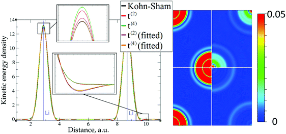 | ||
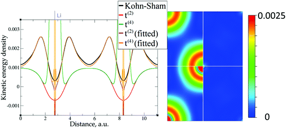
| Fig. 6 Kinetic energy density for lithium (3 valence electrons), computed with Kohn–Sham DFT and with different gradient approximations for the KEDF (applied to the KS DFT density). On the left – the line along direction {1 1 1}; on the right – the projection of plane {1 0 1} with absolute differences between KEDs of different gradient approximations and the Kohn–Sham KED: upper left quadrant – formal t(2)(r), upper right quadrant – fitted t(2),fit(r), bottom left quadrant – formal t(4)(r), bottom right quadrant – fitted t(4),fit(r). For better visibility the scale for the 2D plot is different from the one used for Fig. 5. Atom positions are in the corners with large KED variation. The kinetic energy density unit is Ha per Bohr3. | ||
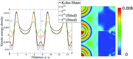
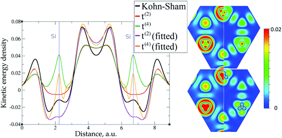
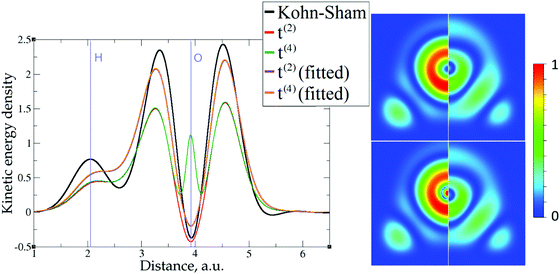
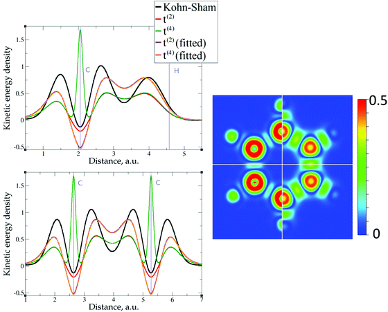
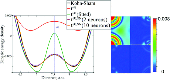
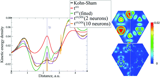
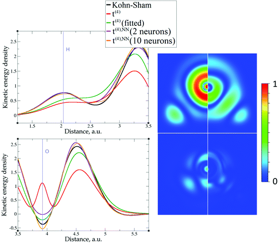
The 1D plots of kinetic energy densities in selected directions are shown in Fig. 3–10 together with 2D plots of errors vs. KS KEDs with different models. The difference between the 2nd- and the 4th-order expansions is noticeable mostly in the regions close to nuclei, where the corresponding valence electron densities tend to their minimum. This tendency is pseudopotential-dependent and may give rise to numeric instabilities (as is clearly seen in the case of Li and Mg) discussed in the next subsection. From the curves of kinetic energy densities, it is seen that the inclusion of 4th-order terms t4(r) affects mostly the near-nuclei regions, significantly increasing the values of the KED there. It is often the case when the local minimum of the t(2)(r) formal expansion turns in this way to a local maximum of the formal t(4)(r) expansion. We use “formal” for the expansions of eqn (2)–(4), as opposed to the tuned expansions presented below. While in some cases this behavior is in accordance with the general shape of the KS kinetic energy density curves, there are cases where it is not – for example, the water molecule and benzene, Fig. 9 and 10, respectively. It is worth noting that the distributions of the formal t(2)(r) for the considered molecules seem in line with the distributions which were investigated for |∇n(r)|2/n(r) in the case of C3H4 and SiH4 molecules in ref. 37. In the regions of space far from nuclei, the formal t(2)(r) and t(4)(r) expansions tend to match. Table 2 clearly shows that for the light metals considered here, the 4th order expansion does improve the KED, for the covalently bonded bulk Si, there is no improvement in the total RMSE, and in the molecular systems, there is significant worsening of the quality of the KED upon inclusion of the 4th order terms. In both Si and the molecules, t(4)(r) fails in regions where the data are scarce (see Fig. 1).
| Expansion | Al | Mga | Lib | Si | H2O | C6H6 |
|---|---|---|---|---|---|---|
| a 10 valence electrons. b 3 valence electrons. | ||||||
| t (2)(r) | 2.07 × 10⁻² | 3.03 | 1.01 | 1.65 × 10⁻² | 2.05 × 10⁻² | 2.06 × 10⁻² |
| t (4)(r) | 1.17 × 10⁻² | 1.78 | 0.95 | 1.67 × 10⁻² | 1.65 × 10⁻¹ | 8.53 × 10⁻² |
| Fitted t(2),fit(r) | 8.19 × 10⁻⁴ | 1.01 × 10⁻¹ | 4.78 × 10⁻³ | 3.96 × 10⁻³ | 1.60 × 10⁻² | 1.94 × 10⁻² |
| Fitted t(4),fit(r) | 3.33 × 10⁻⁴ | 2.43 × 10⁻² | 2.26 × 10⁻³ | 3.57 × 10⁻³ | 1.60 × 10⁻² | 1.94 × 10⁻² |
Overall, one cannot conclude that the formal t(4)(r) expansion systematically improves over the formal t(2)(r) expansion. The failure of the formal density gradient expansions to reproduce quantitatively the KS kinetic energy density was expected. It was also expected that the expansions would perform much better for light metals with a more uniform density than for molecules. Below, we explore possibilities of using t(4)(r) as a basis for further improvements.
The role of pseudopotentials
Among the examples covered in this work, there are two cases with numerical instability of gradient density expansions in close proximity to the nuclei: Mg with two valence electrons (Fig. 3), and Li with 1 valence electron (Fig. 5). The reason is small, near-zero, values of valence electron densities at the nuclei that affect the terms with electron densities of different powers in denominators. What is important is not just the low density but how it tends to the minimum, which is reflected in the respective electron density derivatives. Indeed, considering, for example, the water molecule (Fig. 9), one sees that there are no instabilities in the regions far from the nuclei, where the electron density also reaches near-zero values but in a more gradual way.The shape of the valence electron density is governed by the respective pseudopotential. For modern non-local pseudopotentials, it is often the case that the s-electron pseudopotential channel is characterized by a relatively high positive value (on the order of 1 a.u. and higher) at the origin (see, for example, Fig. 11 for a GTH pseudopotential for Mg with 2 valence electrons). This channel also dominates local PPs for elements with s-only valence shells.70,71 The density then decays exponentially fast and steeply towards the nucleus. This forces the expressions with different powers of electron density in the denominator and powers of derivatives in the numerator to become numerically unstable around the nucleus. Sometimes, this affects even the numerically stable representation of T2, without the electron density in the denominator,69
 | (9) |
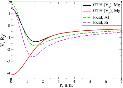 | ||
| Fig. 11 s- and p-channels of a GTH pseudopotential for Mg with 2 valence electrons as well as local pseudopotentials for Al and Si.72 | ||
A similar issue, together with what was called by the authors an “uncertainty” of pseudopotentials, was reported by Karasiev and Trickey70 in relation to GGA73 and mcGGA74 functionals with the square of the reduced density as one of the components. For the mcGGA functional, this was attributed, at least partially, to the imposition of the positivity constraint.75 Later a way to overcome this problem in the context of GGA-type KEDFs was proposed.76
However, the issue we face looks to be purely technical; it is related to elements with only s-electrons in valence shells and is not dependent on any constraints. Indeed, the presence of the contribution from p valence electrons, for which the corresponding valence p electron pseudopotential channel is normally negative at the origin, is able to make the total valence electron density approach its minimum at the nucleus in a more gradual way. For example, no numerical instabilities appeared in the case of aluminum with three valence electrons (see Fig. 7), whose valence shell differs from that of Mg only by one p electron.
This numerical issue is resolved by increasing the number of explicitly considered electrons (so call “semi-core” pseudopotentials), for example, by using 10 electrons for Mg or 3 electrons for Li (see Fig. 4 and 6). In addition, there is no formal reason that would prohibit producing pseudopotentials that would force the s-electron valence densities to approach a minimum at the nucleus more gradually, thus enabling the consideration of only the valence s-states for alkali and alkaline earth metals. This is something that pseudopotential development for OF-DFT might consider in the future.
In summary, with the proper choice of the pseudopotential, in the framework of solid-state periodic calculations, the t(4)(r) expansion terms remain continuous everywhere and can serve as a base for further searching for an accurate approximation to the kinetic energy density.
NN training on KEDs of individual compounds
For individual fits, we used a single hidden layer neural network, which is a universal approximator.45,77,78 The number of training and test points was chosen to be approximately equal to one-third of the total number of sampling points each.Coefficient fitting
The utility of different-order gradient expansions can be explored by fitting of the corresponding term coefficients for each of the studied systems. This helps to answer the question if it is possible at all to find a linear set of coefficients that allows for a close approximation to the KS kinetic energy density for a broad range of compounds. Fitting of the coefficients results in much improvement over the formal t(2)(r) and t(4)(r) gradient density expansions, which can be detected even visually, as can be seen in Fig. 3–10. The most successful cases are elemental metals – Li, Mg, and Al. For them, fitted t(4),fit(r) in general is able to produce a better fit to τKS(r) than fitted t(2),fit(r). That is most noticeable in the interatomic region in Al (Fig. 7) and near-nuclear regions in Mg and Li (Fig. 4 and 6, respectively). Only the fitted t(4),fit(r) was able to reproduce a local minimum of τKS(r) for Mg (10 valence electrons) and Li (3 valence electrons) in regions of both large and small values of τKS(r) (see the inserts of Fig. 4 and 6, respectively). Although there are some regions where t(4),fit(r) seemingly performs worse than t(2),fit(r), in other regions, significant improvements are observed. It might be that there is not enough freedom in linear fitting to achieve improvements with z1–5(r) terms in all regions of space. The performance may also be affected by data distribution. Nevertheless, the overall fitting performance of t(4)(r) is (necessarily) better, as can be seen from the RMSE on the entire test set (Table 2). However, the coefficient fitting procedure was not able to fix the above-discussed numerical instabilities associated with pseudopotentials.As expected, for molecules and Si, the fit performs worse than for elemental metals, which questions the suitability of gradient expansions to reproduce both near-nuclei and covalently bonded regions. Moreover, for these compounds t(4),fit(r) does not improve the KED much over t(2),fit(r), contrary to the elemental metals.
It is worth noting that in the case of elemental metals (Li, Mg, and Al) the systematic attempt of the fitting procedure makes the z1(r) contribution negative (in the range from −0.05 to −0.20, here and below this refers to scaled KED values), when only the valence electrons are considered (1, 2 and 3 electrons for Li, Mg, and Al, respectively). The z1(r) contribution becomes positive when 1s (Li) or 2s2p (Mg) states are included in the pseudopotential. However, in that case, the value of the z1 coefficient is still significantly smaller than in the formal expansion (of around 0.05 for Li and 0.96 for Mg). In contrast, the z2(r) contribution becomes in general larger – from 1/9 in the formal expansions to 0.95–1.27 in the case of Al and Li and even 4.28 for Mg with 2 valence electrons. This tendency is also observed for other systems – the z2(r) contribution is always larger than in the formal expansion, and the z1(r) contribution is smaller and always positive. This is in line with suggestion that the Thomas–Femi term includes a part of the KED incorrectly, and that the performance of gradient density expansions might be improved by subtracting this part.79,80 It has also been shown that the usage of a larger fraction of z2(r) in the 2nd order gradient expansion gives closer total energies to Hartree–Fock references in the case of noble gas atoms (Ne, Ar, Kr, and Xe)81 and better binding energies in the case of di-atomic molecules (H2, N2, O2, HF and CO).82 Overall, the test on atoms up to the 3rd row inclusive suggests that the higher the fraction of z2(r), the lower the fraction of z1(r) that should be used in order to reproduce correctly the total energy; however, this dependence is not linear.83 It is hard to discern a common pattern in the behavior of the coefficient for z3–5(r) terms. The terms might have either positive or negative sign depending on the compound. However, what is common is that their contributions to the KED are one–two orders of magnitude larger than in the formal expansion.
In spite of the apparent improvements offered by the fitting procedure, the results for molecules and systems with localized electrons (Si) remain unsatisfactory. On the other hand, these tests show that systems with delocalized electrons (metals) and a simpler topology of τKS(r) can be quite well reproduced. The next step for the improvement of gradient density expansions is to go beyond coefficient tuning, and this is considered next.
Non-linear fitting with neural networks using terms of the 4th order expansion as density-dependent variables
In the previous section, it was shown that the 4th order expansion either results in a better match to τKS(r) or does not perform worse than the fitted 2nd order expansion. For covalently bound systems, however, fitted t(4),fit(r) did not result in an improvement in the KED over fitted t(2),fit(r). Therefore, for non-linear fitting of KEDFs by training neural networks we included all z1–5(r) functions in the input vector. Table 3 lists RMSE errors in the kinetic energy density integrated over test data for NN fits using different numbers of hidden neurons. There is a significant improvement in the KE over linearly tuned coefficients. This improvement is obvious also for the covalently bound bulk Si and water and benzene molecules. The most significant improvements are for Al and Mg where the RMSE with 12 non-linear neurons becomes smaller by an order of magnitude than the RMSE achieved with linear fitting. For other compounds, the improvements are also significant, leading to 4–5 times better test set RMSEs.| N n | Al | Mga | Lib | Si | H2O | C6H6 |
|---|---|---|---|---|---|---|
| a 10 valence electrons. b 3 valence electrons. | ||||||
| 2 | 1.79 × 10⁻⁴ | 6.43 × 10⁻³ | 1.23 × 10⁻³ | 2.73 × 10⁻³ | 4.57 × 10⁻³ | 1.50 × 10⁻² |
| 4 | 3.86 × 10⁻⁵ | 3.04 × 10⁻³ | 9.24 × 10⁻⁴ | 2.16 × 10⁻³ | 3.55 × 10⁻³ | 1.27 × 10⁻² |
| 6 | 2.07 × 10⁻⁵ | 1.55 × 10⁻³ | 1.04 × 10⁻³ | 1.47 × 10⁻³ | 3.42 × 10⁻³ | 1.22 × 10⁻² |
| 8 | 1.34 × 10⁻⁵ | 1.41 × 10⁻³ | 1.00 × 10⁻³ | 1.62 × 10⁻³ | 3.62 × 10⁻³ | 1.15 × 10⁻² |
| 10 | 1.41 × 10⁻⁵ | 8.38 × 10⁻⁴ | 5.78 × 10⁻⁴ | 1.35 × 10⁻³ | 3.06 × 10⁻³ | 1.19 × 10⁻² |
| 12 | 1.27 × 10⁻⁵ | 7.26 × 10⁻⁴ | 1.01 × 10⁻³ | 7.07 × 10⁻⁴ | 3.39 × 10⁻³ | 1.19 × 10⁻² |
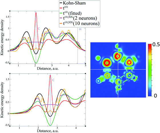
As expected, the fitting precision is systematically increased with the increase of the number of neurons Nn for small Nn. For covalently bound systems, the test error can increase for Nn larger than 10. This likely has to do with the distribution of the data. While the total dataset contains millions of entries (i.e. a much larger number than the number of NN parameters thus ensuring that NN coefficients are not overfitted), there are few data in specific ranges of the KED (Fig. 1). The effect of non-linear fitting can be visually observed in Fig. 12–17. For metals, the NN-based KED follows τKS very accurately. For water and benzene molecules, the NN-based KED appears to follow τKS very accurately in regions where there are sufficient training data; it fails badly in regions of few data. Data distribution therefore appears to be a major issue in covalently bound systems. A way to improve the fitting was demonstrated in the case of Si (see ‘Methods’) – the ‘poorly’ represented regions of KED values can be replenished from another denser point grid that is built just around these regions (atoms or molecules). It should be noted that a simple increase of the grid resolution for the whole simulation cell is not a solution, since the ‘problematic’ regions of KED values will be still ‘poorly’ represented relatively to other regions, and the corresponding histogram of the KED value distribution will remain strongly non-uniform. More advanced techniques to deal with data distribution likely have to be developed for successful application of gradient expansion based KEDFs in such systems.
Joint NN training on KEDs of several compounds
The task of producing a transferable KE functional implies the necessity of performing simultaneous training over multiple species of interest (subsequently this procedure will be referred to as “joint training”). Since the accuracy of individual training for molecules was considerably worse that the accuracy achieved with the solid compounds (although not worse than the ML KED functionals which were recently reported54) we decided to perform joint training for Al, Li, Mg and Si. Further, our aim was to reach an accuracy of joint training which is comparable to that with the individual non-linear fits (thus of 10−5 Ha per Bohr3 for simple metals and 10−4 Ha per Bohr3 for Si, see Table 3). From this point of view, the latter are playing the role of a reference for reachable accuracy.As has been shown above, the difficulty of the fit is compounded by the data distribution. While for the individual NN fits the considered above 3D sampling was dense enough, the joint training required much denser meshes and seemingly larger neural networks which can severely increase the computational cost. One way to get around this problem is to make use of the symmetry of the unit cells, i.e. to replace 3D data with 2D data, which can be extracted from the corresponding crystallographic planes. Obviously, the properties (like the electron density and KED) can be sampled much more densely over planes than over 3D cells, while the total number of sampling points can be much less. In our investigation we decided to include into training sets two planes from each of the solid compounds – thus {100} and {110} planes were chosen in the case of Al, Li and Si, and {0001} and {11−20} planes were chosen for Mg. The sampling density of the planes was 0.01 Bohr per point and 1/5 of the total number of points were taken as training data.
The next important point is data compatibility – it appeared that mixing of large-core and small-core elements can make the training procedure much more error prone and more inclined to overfitting. Therefore, we decided to take pseudopotentials with 2 valence electrons for Mg and 1 valence electron for Li. Keeping in mind the pseudopotential issue that was described in section “The role of pseudopotentials”, we have taken the corresponding FHI large-core pseudopotentials, which are seemingly less affected by it than the GTH pseudopotentials.
The resulting RMSEs for several neural networks are presented in Table 4. We would like to stress that the corresponding RMSEs were calculated with respect to the 3D data in the cube files, which were described in the “Introduction” (i.e. beyond the 2D planes which were used for NN training).
| [Nn] | Al | Mga | Lib | Si |
|---|---|---|---|---|
| a 2 valence electrons. b 1 valence electron. | ||||
| [60] | 3.17 × 10⁻⁴ | 2.63 × 10⁻⁴ | 1.56 × 10⁻⁴ | 1.04 × 10⁻³ |
| [30 30] | 1.28 × 10⁻⁴ | 2.10 × 10⁻⁴ | 1.37 × 10⁻⁴ | 1.16 × 10⁻³ |
| [20 20 20] | 9.23 × 10⁻⁵ | 1.91 × 10⁻⁴ | 2.42 × 10⁻⁵ | 1.04 × 10⁻³ |
| [80] | 2.87 × 10⁻⁴ | 1.70 × 10⁻⁴ | 6.33 × 10⁻⁵ | 9.94 × 10⁻⁴ |
| [40 40] | 1.10 × 10⁻⁴ | 1.56 × 10⁻⁴ | 2.05 × 10⁻⁵ | 1.02 × 10⁻³ |
| [20 20 20 20] | 8.00 × 10⁻⁵ | 2.45 × 10⁻⁴ | 1.82 × 10⁻⁵ | 1.32 × 10⁻³ |
| [100] | 2.81 × 10⁻⁴ | 9.71 × 10⁻⁵ | 5.88 × 10⁻⁵ | 1.01 × 10⁻³ |
| [50 50] | 1.16 × 10⁻⁴ | 4.90 × 10⁻⁵ | 2.21 × 10⁻⁵ | 1.14 × 10⁻³ |
| [25 25 25 25] | 7.56 × 10⁻⁵ | 6.99 × 10⁻⁵ | 1.82 × 10⁻⁵ | 1.69 × 10⁻³ |
| [20 20 20 20 20] | 3.90 × 10⁻⁵ | 2.26 × 10⁻⁵ | 1.54 × 10⁻⁵ | 1.65 × 10⁻³ |
It is seen that to get an accuracy which is comparable to the accuracy of the individual fits, one should take 60 or more neurons. As expected, the increase of the number of neurons within one hidden layer (thus going from [60] to [80] and [100]) can improve the average (over compounds and data) fit accuracy. This average however hides the fact that the KED may deviate substantially from the target and or exhibit oscillatory behavior is parts of the space, see Fig. 18, which makes the resulting KED functionals not suitable for self-consistent density minimization procedures. This is an indication of overfitting caused by data distribution (as the number of NN parameters is much smaller than the number of training data). This can be palliated by using multiple hidden layers. Indeed, the NN configuration [20 20 20] (that is in total 60 neurons, which are distributed evenly over 3 hidden layers) shows the same average accuracy as the NN with configuration [100] (that is, in total 100 neurons in one hidden layer). In general, for all considered total numbers of neurons, we find that 2 hidden layers are more advantageous over one hidden layer, and 3 or 4 hidden layers are more advantageous than 2 hidden layers. As shown in Fig. 18, the KED functionals which were produced with 4 hidden layers look much smoother. Even when the respective RMSE is not improved, the advantage of several hidden layers is apparent – see for example Si. The RMSE for 80 neurons in one hidden layer is 9.94 × 10⁻⁴ a.u. while the RMSE for 80 neurons in 4 hidden layers ([20 20 20 20] in Table 4) is slightly larger (1.32 × 10⁻³ a.u.); however, the local behavior in the latter case is much better. Of course, the number of NN parameters is significantly higher with a multilayer NN that achieves a similar test set RMSE as a single hidden layer NN (e.g. 560 parameters for [80] and 1400 parameters for [20 20 20 20]). The numbers of parameters, however, remain much smaller than the number of data. We use the multilayer NN not to decrease further the RMSE by increasing the number of parameters but to palliate the overfitting induced by the very non-uniform data distribution.
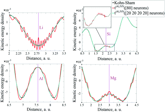 | ||
| Fig. 18 Kinetic energy density from non-linear fitted t(4),NN(r) for: top left – Li, top right – Si, bottom left – Al, bottom right – Mg. The kinetic energy density unit is Ha per Bohr3. | ||
In principle, it must be possible to produce an accurate KEDF using this approach for a larger pool of compounds. We would like to emphasize several points that can greatly (as was shown above) facilitate the accuracy of such machine-learned functionals:
• It is necessary to pay close attention to the data distribution and data selection for training. The KED shows a very uneven distribution for all compounds. Data selection can be improved by some effective histogram equalization procedure or by sampling the respective data as close as possible.
• To reduce the computational costs, a sampling over crystallographic planes can be used instead of 3D sampling.
• The utilization of several hidden layers (ideally more than 2) looks important to prevent overfitting and to produce smooth KED in all space.
• There is no need to use extremely large neural networks, 15–20 neurons per compound should be enough to reach a decent accuracy.
Energy evolution in the self-consistent minimization procedure
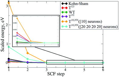
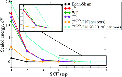
In order to verify the performance of the T(4)-based functional in a self-consistent minimization procedure in OF-DFT, the formal T(4) expansion and ML-fitted KEDFs were implemented in PROFESS 3.0. The electron densities from each SCF optimization step in a Kohn–Sham minimization procedure (done in Abinit) were taken as inputs, and the respective total energies with T(2), T(4), and ML KEDFs, and Wang–Teter (WT)84 KEF were calculated. The results for aluminum and silicon are presented in Fig. 19 and 20, respectively. Molecules were not considered in this test due to the lack of available local pseudopotentials for hydrogen, carbon and oxygen to perform the calculation in PROFESS and because the T(4)-based approximations performed too poorly for molecules, as shown above.The main conclusion is that the formal T(2) expansion, the formal T(4) expansion and non-linear NN fits all show a monotonic decrease of energy along KS-DFT SCF steps, as does the WT KEDF, even in the case of Si. This is encouraging. However, we were unable to perform a complete SCF minimization either with the formal T(4) expansion or with the fits. Depending on different input electron densities (whether uniform, which is the default initialization in PROFESS, or taken from Kohn–Sham calculations), the optimization procedures ended up after only 3–4 optimization steps stuck in high-energy local minima, which were close to those calculated from uniform distribution of charges (the latter are used for initialization). The resulting kinetic energy densities experienced unsmooth behavior in near-nuclei regions that points toward numerical instabilities during the density optimization procedure. It is, however, possible that this error happened due to local pseudopotentials in OF-DFT calculations, since the numerical instabilities in our work were caused exclusively by pseudopotentials, and the pseudopotentials for Al and Si available in PROFESS do have a shape (a “wall” towards the nucleus, see Fig. 11) which we showed above cause instabilities in the terms of the gradient expansion.
Conclusions
We explored the possibility of using the 4th order expansions of electron density as a base for the search for orbital-free approximations to the KED. It was previously suggested that due to the electron densities of different powers in denominators, these expansions would be numerically unstable. However, we have shown that with the proper choice of pseudopotential, the corresponding KED curves from 4th-order expansions remain continuous everywhere, including low-density regions. For simple bulk metals Li, Al, and Mg, the 4th order expansion of the electron density with fitted coefficients is already able to reproduce the Kohn–Sham KED well. This is not the case for covalently bound systems such as bulk Si and molecular H2O and C6H6 tried here.A closer match to the Kohn–Sham KED, including for systems with localized electrons (covalent bonds), can be obtained by using the 4th order expansion terms as inputs for non-linear regression, which we performed using neural networks. Our NN fits to each compound resulted in extremely low fit and test set RMSE values without overfitting of NN coefficients. For this purpose, small single layer NNs serve well, since they are already universal approximators.
For covalently bonded compounds, the quality of the 4th order expansion is strongly affected by the non-uniformity of KED distributions. A better representability of the fitting data could be achieved by consideration of problematic regions (generally near-nuclei regions) on denser grids. More advanced techniques to deal with data distribution should be explored.85
The evolution of total energies from T(4)-based expansions, calculated with Kohn–Sham electron densities as inputs, is seemingly in accordance with Kohn–Sham energies – the minimum of the electron density corresponds to the minimum of the total energy. However, the elaboration of better local pseudopotentials might be required in order to use T(4) expansions or their parts in SCF minimization procedures, which in our tests were not convergent. We thus hope that these results will be useful in the development of new kinetic energy functionals and pseudopotentials for orbital-free DFT.
Further, the issue of non-uniformity of KED distributions greatly complicates NN training to KEDs of several compounds simultaneously, and, as consequence, the task of producing a reliable transferable KE functional. We have shown that good joint fits can be obtained by densely sampling training data on planes in combination with the usage of several hidden layers in the NN architecture. We would like to point out that this does not question the quality of a single hidden layer network as a universal approximator, since this holds only for infinitely dense sampling.
The main result is that it is possible to obtain a very close match to orbital-based KEDs using machine learning tools, both for individual compounds (including molecules) and joint training. We achieved this with the terms of the T(4) expansion as density-dependent inputs. The corresponding RMSEs were extremely low, on the order of 1 mHa per Bohr3 (for Si) and less (for simple metals). To the best of our knowledge, this is the most precise NN fitting to KEDs of real systems so far.
It would also be of great interest to apply a similar NN approach to other types of systems like ionic solids and transition metals, that might not be harder than the covalent systems.
Conflicts of interest
There are no conflicts to declare.Acknowledgements
This work was supported by the Ministry of Education of Singapore (AcRF Tier 1 grant). We thank Daniel Koch for help with some calculations and Michele Pavanello, Emily Carter, Paul Ayers, and Hiromi Nakai for discussions.References
- P. Hohenberg and W. Kohn, Phys. Rev., 1964, 136, B864 CrossRef.
- D. Sholl and J. A. Steckel, Density Functional Theory: A Practical Introduction, Wiley, 2009 Search PubMed.
- W. Kohn and L. J. Sham, Phys. Rev., 1965, 140, A1133 CrossRef.
- Recent Progress in Orbital-free Density Functional Theory, ed. T. A. Wesolowski and Y. A. Wang, World Scientific, 2013 Search PubMed.
- Y. A. Wang, N. Govind and E. A. Carter, Phys. Rev. B: Condens. Matter Mater. Phys., 1998, 58, 13465 CrossRef CAS.
- Y. A. Wang, N. Govind and E. A. Carter, Phys. Rev. B: Condens. Matter Mater. Phys., 1999, 60, 16350 CrossRef CAS.
- B. Radhakrishnan and V. Gavini, Philos. Mag., 2016, 96, 2468 CrossRef CAS.
- S. Das, M. Iyer and V. Gavini, Phys. Rev. B: Condens. Matter Mater. Phys., 2015, 92, 014104 CrossRef.
- M. Chen, X.-W. Jiang, H. Zhuang, L.-W. Wang and E. A. Carter, J. Chem. Theory Comput., 2016, 12, 2950 CrossRef CAS PubMed.
- W. C. Witt, B. G. del Rio, J. M. Dieterich and E. A. Carter, J. Mater. Res., 2018, 33, 777 CrossRef CAS.
- C. Huang and E. A. Carter, Phys. Rev. B, 2010, 81, 045206 CrossRef.
- D. A. Kirzhnits, Sov. Phys.-JETP, 1957, 5, 64 Search PubMed.
- L. H. Thomas, Proc. Cambridge Philos. Soc., 1927, 23, 542 CrossRef CAS.
- E. Fermi, Rend. Accad. Naz. Lincei, 1927, 6, 602 CAS.
- C. F. V. Weizsäcker, Z. Phys., 1935, 96, 431 CrossRef.
- C. H. Hodges, Can. J. Phys., 1973, 51, 1428 CrossRef.
- D. R. Murphy, Phys. Rev. A: At., Mol., Opt. Phys., 1981, 24, 1682 CrossRef CAS.
- W.-P. Wang, R. G. Parr, D. R. Murphy and G. A. Henderson, Chem. Phys. Lett., 1976, 43, 409 CrossRef CAS.
- D. R. Murphy and W.-P. Wang, J. Chem. Phys., 1980, 72, 429 CrossRef CAS.
- E. Clementi and C. Roetti, At. Data Nucl. Data Tables, 1974, 14, 177 CrossRef CAS.
- C. Lee and S. K. Ghosh, Phys. Rev. A: At., Mol., Opt. Phys., 1986, 33, 3506 CrossRef CAS.
- N. L. Allan, C. G. West, D. L. Cooper, P. J. Grout and N. H. March, J. Chem. Phys., 1985, 83, 4562 CrossRef CAS.
- N. L. Allan and D. L. Cooper, J. Chem. Phys., 1986, 84, 5594 CrossRef CAS.
- P. E. Blöchl, Phys. Rev. B, 1994, 54, 17953 CrossRef.
- J. Lehtomäki, I. Makkonen, M. A. Caro, A. Harju and O. Lopez-Acevedo, J. Chem. Phys., 2014, 141, 234102 CrossRef PubMed.
- Y. Tal and R. F. W. Bader, Int. J. Quantum Chem., 1978, S12, 153 Search PubMed.
- E. W. Pearson and R. G. Gordon, J. Chem. Phys., 1985, 82, 881 CrossRef CAS.
- J. P. Perdew, M. Levy, G. S. Painter, S. Wei and J. B. Lagowski, Phys. Rev. B, 1988, 37, 838 CrossRef CAS.
- A. E. DePristo and J. D. Kress, Phys. Rev. A: At., Mol., Opt. Phys., 1987, 35, 438 CrossRef CAS.
- A. Sergeev, F. H. Alhabri, R. Jovanovic and S. Kais, J. Phys.: Conf. Ser., 2016, 707, 012011 CrossRef.
- Z. Yan, J. P. Perdew, T. Korhonen and P. Ziesche, Phys. Rev. A: At., Mol., Opt. Phys., 1997, 55, 4601 CrossRef CAS.
- L. Vitos, H. L. Skriver and J. Kollár, Phys. Rev. B, 1998, 57, 12611 CrossRef CAS.
- S. Laricchia, L. A. Constantin, E. Fabiano and F. Della Sala, J. Chem. Theory Comput., 2014, 10(1), 164 CrossRef CAS PubMed.
- L. A. Constantin, E. Fabiano and F. Della Sala, J. Phys. Chem. Lett., 2018, 9, 4385 CrossRef CAS PubMed.
- J. Tao, J. P. Perdew, V. N. Staroverov and G. E. Scuseria, Phys. Rev. Lett., 2003, 91, 146401 CrossRef PubMed.
- J. P. Perdew and L. A. Constantin, Phys. Rev. B, 2007, 75, 155109 CrossRef.
- A. C. Cancio, D. Stewart and A. Kuna, J. Chem. Phys., 2016, 144, 084107 CrossRef PubMed.
- J. Xia and E. A. Carter, J. Power Sources, 2014, 254, 62 CrossRef CAS.
- M. Levy and H. Ou-Yang, Phys. Rev. A: At., Mol., Opt. Phys., 1988, 38, 625 CrossRef.
- S. B. Trickey, V. V. Karasiev and R. S. Jones, Int. J. Quantum Chem., 2009, 109, 2943 CrossRef CAS.
- V. V. Karasiev, D. Chakrabotry, O. A. Shukruto and S. B. Trickey, Phys. Rev. B, 2013, 88, 161108(R) CrossRef.
- S. Smiga, E. Fabiano, L. A. Constantin and F. Della Sala, J. Chem. Phys., 2017, 146, 064105 CrossRef PubMed.
- J. Hollingsworth, L. Li, T. E. Baker and K. Burke, J. Chem. Phys., 2018, 148, 241743 CrossRef PubMed.
- T. M. Mitchell, Machine Learning, MacGraw-Hill Science, 1997 Search PubMed.
- S. Manzhos, X.-G. Wang, R. Dawes and T. A. Carrington, J. Phys. Chem. A, 2006, 110, 5295 CrossRef CAS PubMed.
- S. Manzhos, R. Dawes and T. Carrington, Int. J. Quantum Chem., 2015, 115, 1012 CrossRef CAS.
- B. Kolb, P. Marshall, B. Zhao, B. Jiang and H. Guo, J. Phys. Chem. A, 2017, 121, 2552 CrossRef CAS PubMed.
- G. B. Goh, N. O. Hodas and A. Vishnu, J. Comput. Chem., 2017, 38, 1291 CrossRef CAS PubMed.
- J. C. Snyder, M. Rupp, K. Hansen, L. Blooston, K.-R. Müller and K. Burke, J. Chem. Phys., 2013, 139, 224104 CrossRef PubMed.
- L. Li, J. C. Snyder, I. M. Pelaschier, J. Huang, U.-M. Niranjan, P. Duncan, M. Rupp, K.-R. Müller and K. Burke, Int. J. Quantum Chem., 2016, 116, 819 CrossRef CAS.
- L. Li, T. E. Baker, S. R. White and K. Burke, Phys. Rev. B, 2016, 94, 245129 CrossRef.
- K. Yao and J. Parkhill, J. Chem. Theory Comput., 2016, 12, 1139 CrossRef CAS PubMed.
- F. Brockherde, L. Vogt, L. Li, M. E. Tuckerman, K. Burke and K.-R. Müller, Nat. Commun., 2017, 8, 872 CrossRef PubMed.
- J. Seino, R. Kageyama, M. Fujinami, Y. Ikabata and H. Nakai, J. Chem. Phys., 2018, 148, 241705 CrossRef PubMed.
- X. Gonze, J.-M. Beuken, R. Caracas, F. Detraux, M. Fuchs, G.-M. Rignanese, L. Sindic, M. Verstraete, G. Zerah, F. Jollet, M. Torrent, A. Roy, M. Mikami, P. Ghosez, J.-Y. Raty and D. C. Allan, Comput. Mater. Sci., 2002, 25, 478 CrossRef.
- X. Gonze, B. Amadon, P.-M. Angade, J.-M. Beuken, F. Bottin, P. Boulanger, F. Bruneval, D. Caliste, R. Caracas, M. Cote, T. Deutsch, L. Genovese, P. Ghosez, M. Giantomassi, S. Goedecker, D. R. Hamann, P. Hermet, F. Jollet, G. Jomard, S. Leroux, M. Mancini, S. Mazevet, M. J. T. Oliveira, G. Onida, Y. Pouillon, T. Rangel, G.-M. Rignanese, D. Sangalli, R. Shaltaf, M. Torrent, M. J. Verstraete, G. Zerah and J. W. Zwanziger, Comput. Phys. Commun., 2009, 180, 2582 CrossRef CAS.
- J. P. Perdew, K. Burke and M. Ernzerhof, Phys. Rev. Lett., 1996, 77, 3865 CrossRef CAS PubMed.
- W. Witt, Z. Naturforsch., A, 1967, 22, 92 Search PubMed; M. R. Nadler and C. P. Kempfer, Anal. Chem., 1959, 31, 2109 CrossRef CAS; C. B. Walker and M. Marezio, Acta Metall., 1959, 7, 769 CrossRef; C. R. Hubbard, H. E. Swanson and F. A. Mauer, J. Appl. Crystallogr., 1975, 8, 45 CrossRef.
- S. Goedecker, M. Teter and J. Hutter, Phys. Rev. B, 1996, 54, 1703 CrossRef CAS.
- M. Krack, Theor. Chem. Acc., 2005, 114, 145 Search PubMed.
- M. Fuchs and M. Scheffler, Comput. Phys. Commun., 1999, 119, 67 CrossRef CAS.
- Pseudopotentials for the ABINIT code, https://www.abinit.org/sites/default/files/PrevAtomicData/psp-links/psp-links/gga_fhi.
- Neural Network Toolbox, https://www.mathworks.com/products/neural-network.html.
- Gaussian cube files, http://paulbourke.net/dataformats/cube/.
- R. Gonzalez and R. Woods, Digital Image Processing, Prentice Hall, New Jersey, 2nd edn, 2002 Search PubMed.
- D. Nguen and B. Widrow, Proc. – Int. Jt. Conf. Neural Networks, 1990, 3, 21 Search PubMed.
- K. Levenberg, Q. Appl. Math., 1944, 2, 164 CrossRef.
- D. Marquardt, SIAM J. Appl. Math., 1963, 11(2), 431 CrossRef.
- G. S. Ho, V. L. Ligneres and E. A. Carter, Comput. Phys. Commun., 2008, 179, 839 CrossRef CAS.
- V. V. Karasiev and S. B. Trickey, Comput. Phys. Commun., 2012, 183, 2519 CrossRef CAS.
- W. Mi, S. Zhang, Y. Wang, Y. Ma and M. Miao, J. Chem. Phys., 2016, 144, 134108 CrossRef PubMed.
- C. Huang and E. A. Carter, Phys. Chem. Chem. Phys., 2008, 10, 7109 RSC.
- F. Tran and T. A. Wesolowski, Int. J. Quantum Chem., 2002, 89, 441 CrossRef CAS.
- V. V. Karasiev, S. B. Trickey and F. E. Harris, J. Comput.-Aided Mater. Des., 2006, 13, 111 CrossRef CAS.
- V. V. Karasiev and S. B. Trickey, Adv. Quantum Chem., 2015, 71, 221 CrossRef CAS.
- K. Luo, V. V. Karasiev and S. B. Trickey, Phys. Rev. B, 2018, 98, 041111(R) CrossRef.
- K. Hornik, M. Stinchcombe and H. White, Neural Networks, 1989, 2, 359 CrossRef.
- K. Hornik, Neural Networks, 1991, 4, 251 CrossRef.
- J. Schwinger, Phys. Rev. A: At., Mol., Opt. Phys., 1980, 22, 1827 CrossRef CAS.
- P. K. Acharya, L. J. Bartolotti, S. B. Sears and R. G. Parr, Proc. Natl. Acad. Sci. U. S. A., 1980, 77, 6978 CrossRef CAS.
- W. Yang, Phys. Rev. A: At., Mol., Opt. Phys., 1986, 34, 4575 CrossRef.
- G. K.-L. Chan, A. J. Cohen and N. C. Handy, J. Chem. Phys., 2001, 114, 631 CrossRef CAS.
- L. A. Espinosa Leal, A. Karpenko, M. A. Caro and O. Lopez-Acevedo, Phys. Chem. Chem. Phys., 2015, 17, 31463 RSC.
- L.-W. Wang and M. P. Teter, Phys. Rev. B, 1992, 45, 13196 CrossRef CAS.
- J. Xia and E. A. Carter, Phys. Rev. B: Condens. Matter Mater. Phys., 2015, 91, 045124 CrossRef.
| This journal is © the Owner Societies 2019 |


