
Determining the uncertainty in microstructural parameters extracted from tomographic data†‡
P.
Pietsch
a,
M.
Ebner
a,
F.
Marone
b,
M.
Stampanoni
bc and
V.
Wood
 *a
*a
aLaboratory for Nanoelectronics, ETH Zuerich, Gloriastrasse 35, 8092 Zurich, ETZ H65, ETZ J86, Switzerland. E-mail: ppietsch@iis.ee.ethz.ch; mebner@ethz.ch; vwood@ethz.ch; Tel: +41 44 633 8583 Tel: +41 44 632 4603 Tel: +41 44 432 6654
bSwiss Light Source, Paul Scherrer Institute, 5232 Villigen, WBBA/216, Switzerland. E-mail: federica.marone@psi.ch; marco.stampanoni@psi.ch; Tel: +41 56 310 5318 Tel: +41 56 310 4724
cInstitute for Biomedical Engineering, University and ETH Zuerich, Zuerich, Switzerland
First published on 11th January 2018
Abstract
In the past few years, tomography has emerged as an indispensable tool to characterize and quantify the microstructural parameters of porous media, including lithium ion battery electrodes and separators, fuel cell parts, and supercapacitor electrodes, as well as electrolysis diaphragms. However, tomographic data often suffer from low image contrast between the pore space and the solid phase. As a result, data binarization is error-prone, which translates into uncertainties in the calculated parameters, such as porosity, tortuosity, or specific surface area. We systematically investigate this error propagation on a set of seven commercial negative lithium ion battery electrodes imaged with X-ray tomographic microscopy, and find that, for low porosity electrodes, the selection of binarization criteria can lead to uncertainties in the calculated tortuosity exceeding a factor of two. Our analysis shows that Otsu's interclass variance, which can be determined from a simple and computationally cheap analysis of the histogram of gray values, is a good predictive indicator of the expected uncertainty in the microstructural characteristics.
Introduction
Systems for energy harvesting, conversion, or storage often rely on multiple, heterogeneously distributed phases and materials, which are structurally organized on the micrometer scale. This so-called microstructure influences transport, conversion, and storage, while maintaining the mechanical integrity of the compound. Detailed knowledge of the microstructure is thus crucial to design new compounds with superior effective transport, conversion and storage properties in the energy sector.X-ray tomographic microscopy (XTM) has become the tool of choice to characterize and quantify the microstructure of, for example, lithium ion battery (LIB)1–7 electrodes, LIB separators,8 fuel cell electrodes,9,10 gas diffusion layers,11,12 supercapacitor electrodes,13 electrolysis diaphragms9,14 and reticulate porous ceramics.15 Many XTM experiments aim at condensing the rich microstructure information into a set of few characteristics that can subsequently be attributed to a homogeneous effective medium with similar properties as the original microstructure. The most common characteristics are (i) the porosity ε, which affects both storage and transport properties, (ii) the tortuosity τ, which affects transport properties and is inversely proportional to the medium's effective conductivity or diffusivity, and (iii) the specific surface area As, which controls conversion rates at the material interfaces. In a typical experiment, a sample is imaged ex situ or in situ and, before the microstructural parameters can be calculated,16 the resulting 3D dataset(s) (which contain a range of gray scale values) must be binarized, a procedure whereby voxels (the volume element in 3D, analogous to a pixel in 2D) are assigned one of two distinct gray-scale values and are thereby associated with either the pore space or the active particle phase.
Currently, there is little consistency in data acquisition and image processing procedures among different studies. Unless a ground truth is available for the binarization, the quality of data binarization is typically judged by visual inspection, which is highly subjective. Such a ground truth could, for example, be given by imaging the same sample with an alternative imaging technique that provides significantly better spatial resolution and contrast, albeit often at the cost of invasiveness, increased effort, or smaller sample volumes. This approach has for example been taken in a correlative microscopy study, where the ground truth for the X-ray data was provided by a focused ion beam scanning electron microscopy dataset having higher resolution.17
In this study, we develop a simple method to estimate the errors in common microstructural parameters that are induced by binarization of three-dimensional tomographic data sets.
A typical workflow to binarize tomographic data consists of16 (i) preprocessing the grayscale data by applying a set of filters (e.g. histogram equalization, anisotropic diffusion filters, and noise reduction filters), (ii) thresholding the data, and (iii) postprocessing the binarized data (e.g. a morphological image operation to ensure that a specific type of feature is associated with a given phase).
To systematically investigate how these data processing steps affect the resulting microstructure, we parametrize the binarization process with a variable threshold and filter. The thresholding and filtering methods chosen for this study are discussed in subsequent sections; however, the impact of changing the threshold and filter is shown qualitatively in Fig. 1a. Depending on the chosen threshold and the filter, strikingly different binarized microstructures are obtained from the same raw data. The threshold is a gray scale value that defines which pixels are associated with the pore space and which are associated with the active material. Pixels with a gray scale value smaller than the threshold are associated with the pore space, and those with a gray scale value larger than the threshold are associated with the active material. Increasing the threshold value (moving up the y-axis in Fig. 1a), increases the number of pixels associated with the pore space, resulting in more small-scale features. Filtering can be applied before and after the threshold, and it can be understood as a measure of how strongly the data are modified (e.g., through contrast enhancements, smoothing and noise reductions in the pre- or post-processing step) to facilitate binarization. As shown in Fig. 1a, increasing filtering (moving along the x-axis) eliminates small features from the data.
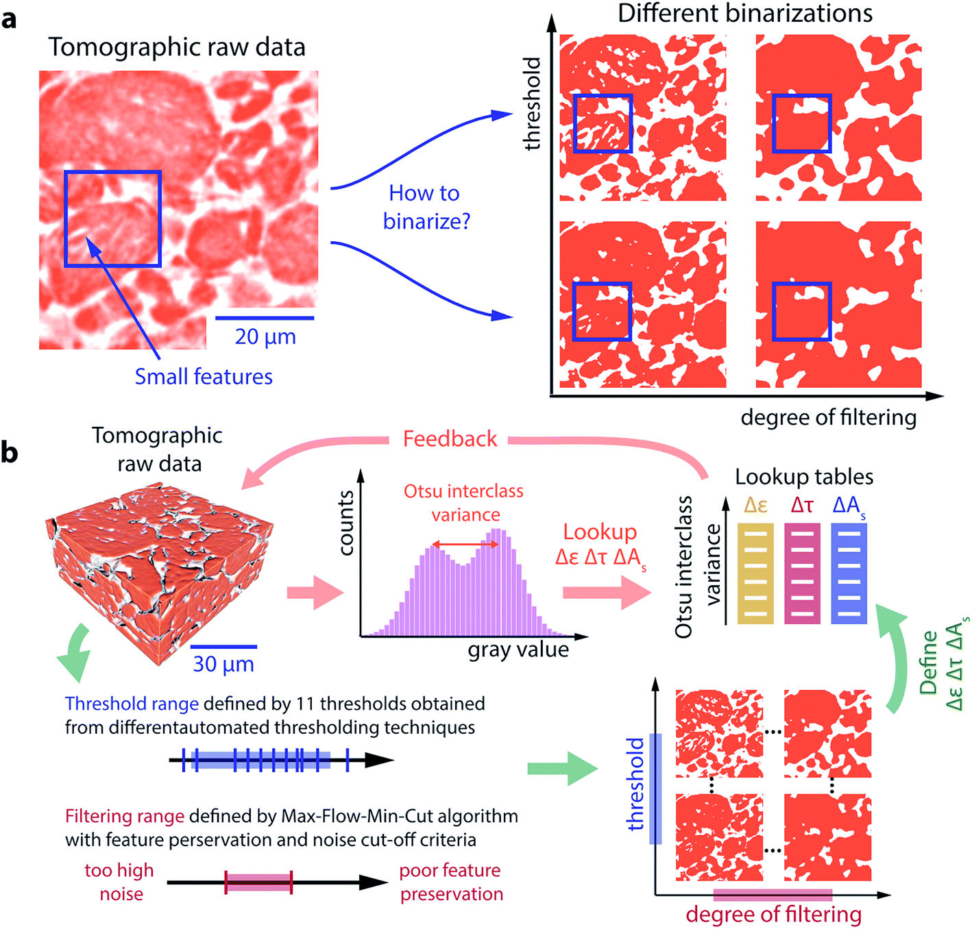 | ||
| Fig. 1 (a) A representative section of a tomogram showing the range of gray scale values present in the raw data. To analyze the microstructure, this raw data must be binarized. Selection of a threshold and a filtering routine will result in different binarized microstructures. A blue rectangle is inserted around a region with small features to guide the eye in assessing the impact of the threshold and filtering parameters on preserving these features. (b) Data processing procedure: for each tomographic raw dataset, 11 thresholds obtained from different histogram-based thresholding algorithms, define the threshold uncertainty range (blue). The degree to which the raw data is smoothed and filtered upon binarization is controlled by the max-flow-min-cut algorithm (see ESI†) with a corresponding filtering range (red) that is defined by noise reduction and feature preservation criteria. The uncertainty ranges of the microstructural characteristics, porosity (ε), tortuosity (τ) and specific surface area (As) are then calculated on the set of binarizations resulting from all threshold – filtering parameter combinations. Repeating this computationally expensive procedure (green route) for different electrodes allows us to establish a lookup table for the expected uncertainty as a function of the Otsu interclass variance, which is a simple histogram based quantity. Once the lookup table is established, simply calculating Otsu's interclass variance from a histogram of the raw data is sufficient to estimate the microstructural uncertainty ranges, allowing for quick feedback to optimize imaging parameters (orange route). | ||
Fig. 1b illustrates the analysis carried out in this paper and how our findings can be implemented to provide error bars on the reported microstructural parameters and/or to optimize imaging parameters on the fly during an XTM imaging beamtime. In the first step, we use the computationally expensive processing path (depicted by the green arrows) to define and evaluate microstructural uncertainties based on strict criteria. In the second step, we make use of our findings to enable a simple and computationally cheap processing path (orange arrows) to quickly estimate microstructural uncertainties and even enable direct feedback and optimization of imaging parameters in real time during an imaging study.
Experimental methods and data processing
For our study, we use graphite-based negative electrodes from seven commercial LIBs. The Samsung 25R6 and E35 power and energy cell anodes and the Sony VTC5 power cell anode are extracted from 18![[thin space (1/6-em)]](https://www.rsc.org/images/entities/char_2009.gif) 650 cells, while the Tesla anode is extracted from a cell of a Tesla Model S car (see ESI†). The Litarion anode and the silicon–graphene–graphite based Nanotek anodes GCA-400 (low capacity) and GCA-2000 (high capacity) are obtained as fresh electrode sheets from the corresponding manufacturers. Understanding the microstructure in the negative electrode is critical for LIB performance and longevity because rapid transport capabilities of the microstructure will mitigate battery degradation due to lithium plating, which was observed during charging at high C-rates.18 Furthermore, graphite-based electrodes pose challenges for XTM imaging, as carbon has a small core charge number, which results in low contrast between the active material and the pore space, as the latter is typically filled with air in an ex situ experiment and with carbon-based electrolytes in an in situ experiment.5 Consequently, subsequent image processing – in particular binarization – is error prone, which directly translates into large uncertainties in the extracted microstructural characteristics.
650 cells, while the Tesla anode is extracted from a cell of a Tesla Model S car (see ESI†). The Litarion anode and the silicon–graphene–graphite based Nanotek anodes GCA-400 (low capacity) and GCA-2000 (high capacity) are obtained as fresh electrode sheets from the corresponding manufacturers. Understanding the microstructure in the negative electrode is critical for LIB performance and longevity because rapid transport capabilities of the microstructure will mitigate battery degradation due to lithium plating, which was observed during charging at high C-rates.18 Furthermore, graphite-based electrodes pose challenges for XTM imaging, as carbon has a small core charge number, which results in low contrast between the active material and the pore space, as the latter is typically filled with air in an ex situ experiment and with carbon-based electrolytes in an in situ experiment.5 Consequently, subsequent image processing – in particular binarization – is error prone, which directly translates into large uncertainties in the extracted microstructural characteristics.
We performed XTM imaging at the TOMCAT beamline at the Swiss Light source in standard attenuation contrast geometry, using a voxel size of 162.5 × 162.5 × 162.5 nm3 (see ESI†). The tomographic data for these electrodes are provided open source.‡19
As previously mentioned, the binarization process is parametrized with two continuously tunable parameters: (i) a threshold that assigns every voxel in the raw data with a gray value larger than the threshold to the foreground and every voxel with a gray value smaller than the threshold to the background and (ii) a filtering parameter that controls the smoothness and feature preservation of the binarization.
To facilitate understanding of the binarization routine applied here, we explain the concepts using a 2D image consisting of pixels. All concepts can be transferred straightforwardly to the case of 3D volumetric image data consisting of voxels.
Applying a threshold to a grayscale image (Fig. 2a) results in a preliminary binarization (Fig. 2b). The assignment of a pixel to either the foreground or the background depends only on its gray value with respect to the threshold level. The hatched pixel in Fig. 2b has been associated with the foreground phase; however, its gray value in the raw data (Fig. 2a) is only slightly above the threshold level, making its affiliation to the foreground or background quite ambiguous. Furthermore, all four of its neighbors belong to the background. Since the size scale of the features in the reconstructed image should be larger than a single pixel, the binarization is likely to be improved by flipping the pixel and associating it with the background phase (Fig. 2c). This is an example of a filtering procedure based on this morphological information that can be used to obtain smoother binarizations with reduced noise.
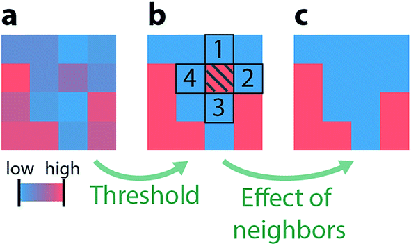 | ||
| Fig. 2 (a) Sketch of a hypothetical grayscale image shown here in false color, where blue represents the background and red represents the foreground. (b) The same image, but binarized by applying a threshold. The hatched pixel had a value larger than the threshold, so it is associated with the foreground even though it is surrounded by pixels (labeled 1–4), which are associated with the background. (c) The same binarized image after flipping the hatched pixel from the image in (b) to adapt the background phase of its four neighbors. | ||
The technical implementation of this is based on the graph cuts theory framework.19 Specifically, we work with a MATLAB based implementation of the max-flow-min-cut algorithm,20–22 which can be downloaded from ref. 23, as discussed in detail in the ESI.†
However, on a qualitative level, one can consider the filtering parameter as a measure of how easily pixels are flipped to adapt the same phase as their neighbors. A small value of the filtering parameter means that the binarization result obtained from thresholding will only be slightly changed. In contrast, a large value for the filtering parameters means that that pixels will adapt to the phase of their neighbors.
Fig. 3 explains the concrete choice of thresholding and filtering ranges used in this work. To define limits on the thresholding axis, we apply 11 different commonly used automated thresholding techniques to the histograms: Otsu,24 Huang,25 isodata,26 peak-average (threshold is defined as the mean of the two peak positions, when the histogram data are fitted with a set of two Gaussians), minerror,27 moments,28 max-entropy,29 triangle,30 Yen,31 Shanbhag32 and Li33 (see ESI†). The different thresholds for a histogram of the Samsung 25R6 electrode data are shown in Fig. 3a. From the distribution of different thresholds, we determine the mean (dashed black) and the standard deviation (light gray area). We define this standard deviation as the range of reasonable thresholds.
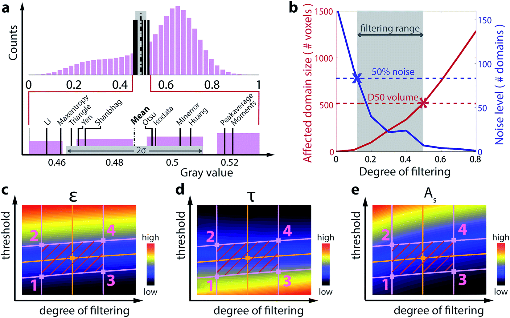 | ||
| Fig. 3 (a) Histogram of gray values (magenta) from one of the electrodes, with thresholds (black lines) computed from 11 reasonable automated thresholding techniques. Zoom-in on the gray value axis makes it easier to identify the exact positions of the different thresholds (black lines). The range of reasonable thresholds is defined as plus/minus one standard deviation (2σ) of the mean (black dashed line) of the different thresholds, which is indicated by the gray bar. (b) Definition of limits for the filtering parameter: the requirement that the noise level (solid blue line) should not exceed 50% of its value at zero filtering (blue dashed line) defines the filtering limit at the low end (indicated by “x”), while the requirement that the size of the biggest flipped domains (solid red line) should not exceed the D50 volume (red dashed line) of either pores or particles defines the filtering limit at the high end (indicated by “*”). Maps of the porosity (c), tortuosity (d) and specific surface area (e) resulting from the binarizations with different threshold and filtering parameter combinations. In each map, the limits of the uncertainty range are indicated by magenta lines, while the orange marker defines the set of binarization parameters that are considered optimal. | ||
A reasonable range of the filtering parameter has to be introduced. To define the lower bound of filtering, we consider the noise level. A minimal amount of filtering should be applied to reduce the amount of noise in the binarizations (“noise reduction criterion”). Since the true spatial resolution is typically on the order of 3 × 3 × 3 voxels, the number of domains with a size smaller or equal to 3 × 3 × 3 voxels is taken as the noise level. As illustrated for the Samsung 25R6 electrode in Fig. 3b, the noise level (blue line) decreases with increasing strength of the filter. We define the lower limit on filtering to be the point (marked by an ‘x’) where the noise level has dropped to 50% of its value at zero filtering (blue dashed line).
In the high filtering limit, the filtering parameter should not exceed a value that erases microstructural features of significant size (“feature preservation criterion”). As the filtering parameter is gradually increased, larger and larger domains will be flipped (i.e. assigned to the phase to which they were not assigned at zero filtering). Tracking the mean size of the 10 largest connected domains in the data that are flipped as a function of the filtering parameter (red curve in Fig. 3b) allows us to set the upper filtering bound where this value equals the minimum of the D50 value of the pore size distribution and the D50 value of the particle size distribution at zero filtering (red dashed line). In other words, we do not allow microstructural features with a size larger or equal to the D50 value of either particle or pore size distribution to be erased by the filtering. According to this criterion, electrodes with small particles and pores allow less filtering than those with larger particles and pores.
We apply a large set of threshold and edge cutting cost binarization parameter combinations within the aforementioned bounds to 350 × 350 × 150 vox3 (57 × 57 × 24 μm3) crops of each of the seven electrodes and calculate the corresponding porosities, tortuosities, and specific surface areas. The maps in Fig. 3c–e plot these values for the Samsung 25R6 electrode. The four magenta lines demark the upper and lower limits on the threshold and the filter parameter as defined above, and the red hatched regions therefore indicate the corresponding range of binarizations. We take the middle point (orange dot) as the parameters for the optimal binarization. As the edge cost parameter is varied, we slightly adapt the threshold limits, such that the porosity remains constant along the boundaries. Absolute positive and negative errors for the different microstructural characteristics can then be defined for each electrode according to:
| Δ+ = max4i=1(Pi − Popt) | (1) |
| Δ− = max4i=1(Popt − Pi) | (2) |
Results & discussion
In Fig. 4a, we show renderings of the seven commercial LIB anodes investigated in this study. Fig. 4b shows the different threshold ranges (red bars) for each electrode as defined by the distance between the horizontal magenta lines on the threshold axis in Fig. 3c–e. The ranges are normalized with respect to the electrode exhibiting the largest range. The blue bars represent the normalized filter parameter ranges and correspond to the distance between the vertical magenta lines on the degree of filtering axis in Fig. 3c–e.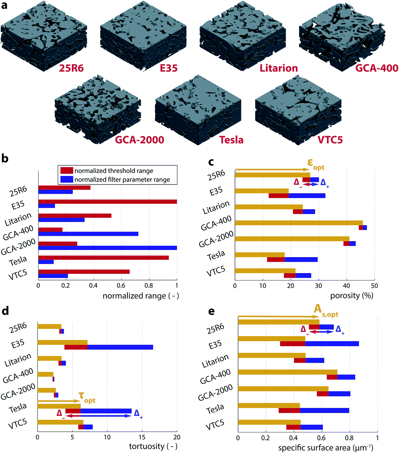 | ||
| Fig. 4 (a) Renderings of the seven commercial LIB negative electrodes investigated in this study. (b) Threshold and filter parameter ranges (respectively, the vertical and horizontal distances between the magenta lines in Fig. 3c–e) for the different electrodes. The ranges are normalized with respect to the highest occurring ranges for the threshold (E35 electrode) and the filtering parameter (GCA-2000 electrode). (c) Porosity (ε), (d) tortuosity (τ), and (e) specific surface area (As) results for the seven different electrodes. The yellow bars show the values resulting from binarization with the parameter combination that is considered optimal (Popt), while the red and blue bars show the negative (Δ−) and positive (Δ+) errors. | ||
There is a negative correlation between the threshold range (red) and the filtering range (blue) in Fig. 4b: for electrodes that are easy to binarize, the threshold uncertainty range is small, while the filtering parameter can be varied in a rather large range without degrading the segmentation quality. On the other hand, a large threshold uncertainty implies that small changes in the filtering parameter significantly affect the binarization results.
The outcomes of the microstructural analysis of the seven electrodes are summarized in Fig. 4c–e. First, as expected from the Bruggeman relation,34 higher porosities correlate with lower tortuosities, as smaller porosities imply thinner and longer diffusion pathways.1,35 Second, as the electrodes show on average rather small porosities, an increase of pore space will also increase the specific surface area, explaining the positive correlation between the two quantities. Most importantly the errors Δ+ and Δ− are rather small for electrodes with large porosities but become very large for small porosity electrodes. In particular, for low porosity electrodes, the computed tortuosity is extremely sensitive to the binarization. For example, in the case of the Tesla and the E35 electrodes, the positive errors in the tortuosities exceed the optimal tortuosity values themselves (i.e. the relative error δ+ exceeds 100%, meaning that the tortuosity is uncertain by a factor of more than two). These results highlight that great care should be taken when low porosity electrodes with weak contrast are binarized for microstructural analysis. The detailed analysis of all seven electrodes is presented in the ESI (Fig. S5–S11†).
The focus of this study is to investigate the uncertainty of microstructural parameters associated with the binarization process; however, it is important to keep in mind other sources of uncertainty, shortcomings and limits associated with XTM imaging. As in most microstructural studies based on X-ray micro-tomographic data,1–7 we compute the porosity, tortuosity and specific surface area values by separating the gray scale data into two phases (i.e., binarizing): the active particle phase (foreground) and the pore phase (background). In lithium ion electrodes, one also finds carbon black and a polymeric binder, which are weakly X-ray absorbing and have feature sizes that typically fall below the spatial resolution limit of X-ray micro-tomography. The carbon black and polymer domain may be present in voxels associated with the particles and in voxels associated with the pores. While the porosity uncertainty arising from this effect is likely to be small due the low weight fraction of these additives in typical commercial negative electrodes (2–4 wt%),36 it could potentially explain the deviations between tortuosity estimates obtained from XTM data and those estimates obtained from electrochemical impedance measurements.37 Furthermore, as has already been discussed elsewhere,6 many surface features of graphite are smaller than the spatial resolution of most XTM setups. Indeed, while our values for the specific surface area of the different electrodes are comparable to other XTM studies of graphite,6,38 they are one to two orders of magnitude below the values obtained from BET surface area measurements (5–100 μm−1).39 Despite this limitation, the trends in specific surface areas provide useful insights into the particle size and shape.
The approach taken above is a computationally expensive and time-consuming way to determine the error in microstructural parameters, as it requires the calculation of binarizations and their corresponding microstructural parameters for many combinations of threshold and filtering parameters. We therefore investigate if our results could be used to develop a criterion, by which the expected uncertainties in the microstructural parameters could be estimated from raw data (e.g. the histogram of gray values).
To find such a criterion, we condense the information contained in a histogram into eight parameters; the mean μ and the standard deviation σ of the overall population as well as the means μj, standard deviations σj and population fractions ωj of the two subpopulations (j = 1, 2) determined by using a single threshold (Fig. 5a), which can be calculated for example from Otsu's automated thresholding method.24
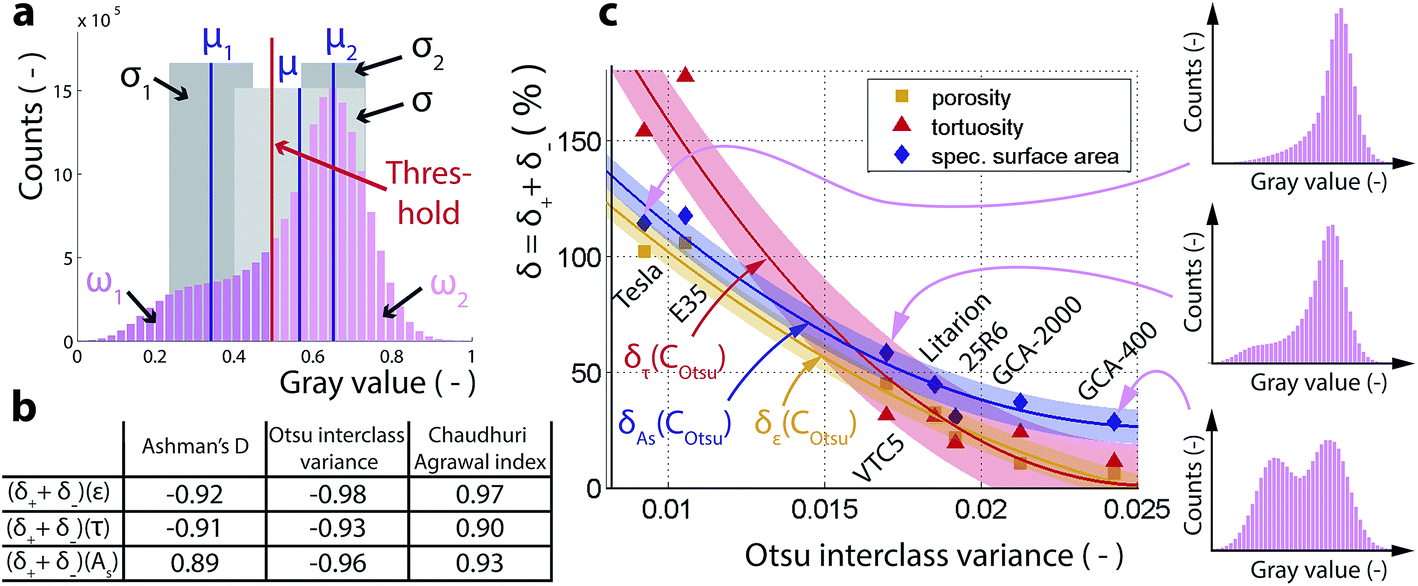 | ||
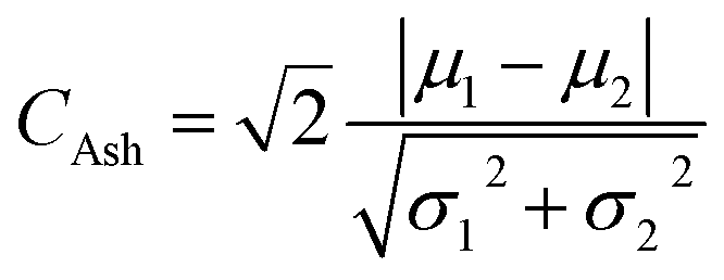
| Fig. 5 (a) Sketch of a bimodal histogram with the means (blue lines), the standard deviations (gray areas) and the weight fractions (magenta bars) associated with the two subpopulations that are obtained by setting a threshold (red line). (b) Pearson’s linear correlation coefficients showing the correlation between the calculated relative errors δ = δ+ + δ− for the different microstructural characteristics with the different approaches to quantify bimodality. (c) Relative errors δ = δ+ + δ− of the porosity (yellow squares), the tortuosity (red triangles), and the specific surface area (blue diamonds) as a function of Otsu's interclass variance for the different electrodes. δε(COtsu), δτ(COtsu) and δAs(COtsu) describe 2nd order polynomial curves for the three microstructural characteristics. The shaded regions correspond to plus/minus one standard deviation of these curves. The magenta histograms on the right are characteristic of the different regimes of the plot. | ||
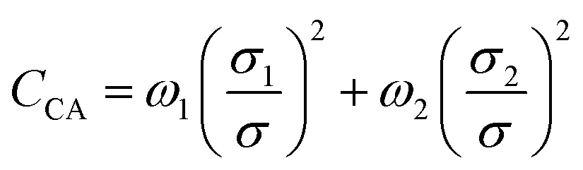
We consider three criteria that are typically used to quantify bimodality and test their correlation with the calculated relative uncertainties δ+ + δ− of the microstructural parameters ε, τ, and As. These are Ashman's D40 (CAsh), Otsu's interclass variance24 (COtsu) and Chaudhuri Agrawal's index41 (CCA), which are defined as:
 | (3) |
| COtsu = ω1ω2(μ1 − μ2)2 | (4) |
 | (5) |
Pearson’s linear correlation coefficients are tabulated in Fig. 5b, and the values close to 1 in absolute value indicate that CAsh, COtsu, and CCA all show a very strong correlation with the microstructural uncertainties.
In Fig. 5c, we plot the relative microstructural uncertainties δ = δ+ + δ− of ε, τ, and As as a function of Otsu's interclass variance COtsu, which shows the most pronounced correlation. The observed trend makes qualitative sense: electrodes with histograms that appear more bimodal by visual inspection (i.e. have more pronounced and separate peaks) show smaller uncertainties in the microstructural characteristics. The curves δε(COtsu), δτ(COtsu) and δAs(COtsu) are empirical 2nd order polynomial representations with the colored shadings representing plus/minus one standard deviation σ:
| δε(COtsu) = 2.31 × 10⁵ × (COtsu)2 − 1.49 × 10⁴ × (COtsu) + 227% ± 6.2% |
| δτ(COtsu) = 6.64 × 10⁵ × (COtsu)2 − 3.37 × 10⁴ × (COtsu) + 428% ± 17.7% |
| δAs(COtsu) = 3.47 × 10⁵ × (COtsu)2 − 1.79 × 10⁴ × (COtsu) + 258% ± 7.3% |
While these equations linking the uncertainties in ε, τ, and As to Otsu's interclass variance do not have a physical meaning, they enable the estimation of those uncertainties from the knowledge of the histogram of gray values. For example, if an Otsu interclass variance of 0.015 is measured for a raw-dataset, the relative errors δ = δ+ + δ− for each of the three microstructural characteristics can be roughly expected in the range 50–100%. With this understanding, imaging parameters (such as the exposure time for a single projection, the number of projections acquired during a tomographic scan, or phase retrieval parameters) can be iteratively altered during a series of XTM experiments until the expected microstructural uncertainties are as low as required. It is important to note, however, that while some imaging parameters (such as the exposure time for a projection) simultaneously improve the accuracy of the sample reconstruction and the image contrast, other parameters improve the contrast (i.e. binarizability) at the expense of reconstruction accuracy. For example, the Paganin phase retrieval filter42 decreases the binarization uncertainty with improved image contrast, but reduces the accuracy of the reconstruction due to lower spatial resolution.5
The uncertainties calculated in this work represent only the uncertainty of the binarization procedure. They do not reflect the accuracy of the XTM reconstructions themselves. For example, with the XTM settings used for these experiments (which result in a voxel edge length of 162.5 nm), nanometer-scale features (such as pores within the graphite particles and the binder-phase) will not be resolved, irrespective of how small the binarization uncertainty is. As described in the ESI,† insight into the accuracy of the reconstruction can be achieved by comparing different types of measurement methods.
However, because the calculated uncertainties refer only to the uncertainty of the binarization procedure and not to the accuracy by which the tomographic reconstructions represent the sample, the relationship between the Otsu interclass variance and the microstructure uncertainties (Fig. 5c) holds independently of the experimental setup and its parameter settings (as long as the histograms are consistently calculated and normalized). XTM reconstructions acquired from two different cathodes imaged with a different X-ray energy and in a different experiment consistently showed very small microstructure uncertainties at large Otsu interclass variances in agreement with our findings on the seven graphite electrodes (see ESI Fig. S4†).
Conclusions
In summary, we investigated the propagation of uncertainties in binarization to uncertainties in the microstructural characteristics by analyzing the XTM data of seven commercial LIB anodes. We found that for low porosity electrodes, ambiguity in binarization can lead to tortuosity uncertainties exceeding a factor of two. We propose a simple relationship for estimating the expected microstructure errors from the Otsu interclass variance calculated from the histogram of the gray values of the raw tomographic data. Compared to the full analysis presented, this presents a computationally facile approach. This approach can be used at a beamline to iteratively optimize the imaging parameters for a specific system. This uncertainty analysis is not limited to LIB negative electrodes, but is applicable to all other systems, where characterization of the microstructure is important for understanding and systematically optimizing devices.Conflicts of interest
There are no conflicts to declare.Acknowledgements
The authors acknowledge the Swiss Light Source for providing measurement time, as well as the Competence Center for Energy and Mobility (P. P.) and the European Research Council (M. E.) for funding.References
- M. Ebner, D.-W. Chung, R. E. García and V. Wood, Adv. Energy Mater., 2014, 4, 1301278 CrossRef.
- M. Ender, J. Joos, A. Weber and E. Ivers-Tiffée, J. Power Sources, 2014, 269, 912–919 CrossRef CAS.
- P. R. Shearing, L. E. Howard, P. S. Jørgensen, N. P. Brandon and S. J. Harris, Electrochem. Commun., 2010, 12, 374–377 CrossRef CAS.
- F. Tariq, V. Yufit, M. Kishimoto, P. R. Shearing, S. Menkin, D. Golodnitsky, J. Gelb, E. Peled and N. P. Brandon, J. Power Sources, 2014, 248, 1014–1020 CrossRef CAS.
- P. Pietsch, D. Westhoff, J. Feinauer, J. Eller, F. Marone, M. Stampanoni, V. Schmidt and V. Wood, Nat. Commun., 2016, 7, 12909 CrossRef CAS PubMed.
- P. R. Shearing, N. P. Brandon, J. Gelb, R. Bradley, P. J. Withers, A. J. Marquis, S. Cooper and S. J. Harris, J. Electrochem. Soc., 2012, 159, A1023–A1027 CrossRef CAS.
- S. J. Cooper, D. S. Eastwood, J. Gelb, G. Damblanc, D. J. L. Brett, R. S. Bradley, P. J. Withers, P. D. Lee, A. J. Marquis, N. P. Brandon and P. R. Shearing, J. Power Sources, 2014, 247, 1033–1039 CrossRef CAS.
- M. F. Lagadec, M. Ebner, R. Zahn and V. Wood, J. Electrochem. Soc., 2016, 163, A992–A994 CrossRef CAS.
- L. Holzer, D. Wiedenmann, B. Münch, L. Keller, M. Prestat, P. Gasser, I. Robertson and B. Grobéty, J. Mater. Sci., 2013, 48, 2934–2952 CrossRef CAS.
- W. K. Epting, J. Gelb and S. Litster, Adv. Funct. Mater., 2012, 22, 555–560 CrossRef CAS.
- J. Eller, J. Roth, R. Gaudenzi, S. Irvine, F. Marone, M. Stampanoni, A. Wokaun and F. N. Büchi, ECS Trans., 2013, 50, 477–486 CrossRef.
- J. Eller, J. Roth, F. Marone, M. Stampanoni, A. Wokaun and F. N. Büchi, ECS Trans., 2011, 41, 387–394 CAS.
- N. Dalili, M. P. Clark, E. Davari and D. G. Ivey, J. Power Sources, 2016, 328, 318–328 CrossRef CAS.
- D. Wiedenmann, L. Keller, L. Holzer, J. Stojadinović, B. Münch, L. Suarez, B. Fumey, H. Hagendorfer, R. Brönnimann, P. Modregger, M. Gorbar, U. F. Vogt, A. Züttel, F. La Mantia, R. Wepf and B. Grobéty, AIChE J., 2013, 59, 1446–1457 CrossRef CAS.
- J. Petrasch, B. Schrader, P. Wyss and A. Steinfeld, J. Heat Transfer, 2008, 130, 32602 CrossRef.
- P. Pietsch and V. Wood, Annu. Rev. Mater. Res., 2017, 47, 451–479 CrossRef CAS.
- R. Moroni, M. Börner, L. Zielke, M. Schroeder, S. Nowak, M. Winter, I. Manke, R. Zengerle and S. Thiele, Sci. Rep., 2016, 6, 30109 CrossRef CAS PubMed.
- J. C. Burns, D. a. Stevens and J. R. Dahn, J. Electrochem. Soc., 2015, 162, A959–A964 CrossRef CAS.
- D. Greig, B. Porteous and A. Seheult, J. Roy. Stat. Soc., 1989, 51, 271–279 Search PubMed.
- J. Yuan, E. Bae, X.-C. Tai and Y. Boykov, 2010 IEEE Conf., 2010, vol. 7, pp. 2217–2224 Search PubMed.
- J. Yuan, E. Bae, X.-C. Tai and Y. Boykov, in Computer Vision - Eccv 2010, Pt Vi, 2010, vol. 6316, pp. 379–392 Search PubMed.
- J. Yuan, C. Schörr and G. Steidl, SIAM J. Sci. Comput., 2007, 29, 2283–2304 CrossRef.
- J. Yuan, Fast continuous max-flow algorithm to 2D/3D image segmentation, https://ch.mathworks.com/matlabcentral/fileexchange/34126-fast-continuous-max-flow-algorithm-to-2d-3d-image-segmentation?focused=5205614%26tab=function, accessed 10 July 2017 Search PubMed.
- N. Otsu, IEEE Trans. Syst. Man Cybern., 1979, 9, 62–66 CrossRef.
- L.-K. Huang and M.-J. J. Wang, Pattern Recogn., 1995, 28, 41–51 CrossRef.
- F. R. Dias Velasco, IEEE Trans. Syst. Man Cybern., 1980, 10, 771–774 CrossRef.
- J. Kittler and J. Illingworth, Pattern Recogn., 1986, 19, 41–47 CrossRef.
- W.-H. Tsai, Comput. Vis. Graph Image Process, 1985, 29, 377–393 CrossRef.
- J. N. Kapur, P. K. Sahoo and A. K. C. Wong, Comput. Vis. Graph Image Process, 1985, 29, 273–285 CrossRef.
- G. W. Zack, W. E. Rogers and S. A. Latt, J. Histochem. Cytochem., 1977, 25, 741–753 CrossRef CAS PubMed.
- J.-C. Yen, F.-J. Chang and S. Chang, IEEE Trans. Image Process., 1995, 4, 370–378 CrossRef CAS PubMed.
- A. G. Shanbhag, CVGIP Graph. Models Image Process., 1994, 56, 414–419 CrossRef.
- C. H. Li and C. K. Lee, Pattern Recogn., 1993, 26, 617–625 CrossRef.
- D. A. G. Bruggeman, Ann. Phys., 1937, 421, 160–178 CrossRef.
- B. Tjaden, S. J. Cooper, D. J. Brett, D. Kramer and P. R. Shearing, Curr. Opin. Chem. Eng., 2016, 12, 44–51 CrossRef.
- I. Urdampilleta, I. de Meatza, K. Ugarte, P. M. Schweizer, N. Loeffler, G.-T. Kim and S. Passerini, Advanced manufacturing processes for low cost greener Li-ion batteries, http://www.greenlionproject.eu/upload/secciones-publicas/iii.electrodes-manufacturing-electrodes-coating_original.pdf, accessed 14 November 2017 Search PubMed.
- J. Landesfeind, J. Hattendorff, A. Ehrl, W. A. Wall and H. A. Gasteiger, J. Electrochem. Soc., 2016, 163, A1373–A1387 CrossRef CAS.
- F. Tariq, V. Yufit, M. Kishimoto, P. R. Shearing, S. Menkin, D. Golodnitsky, J. Gelb, E. Peled and N. P. Brandon, J. Power Sources, 2014, 248, 1014–1020 CrossRef CAS.
- M. Winter, J. Electrochem. Soc., 1998, 145, 428 CrossRef CAS.
- K. A. Ashman, C. M. Bird and S. E. Zepf, Astron. J., 1994, 108, 2348 CrossRef.
- D. Chaudhuri and A. Agrawal, Def. Sci. J., 2010, 60, 290–301 CrossRef.
- D. Paganin, S. C. Mayo, T. E. Gureyev, P. R. Miller and S. W. Wilkins, J. Microsc., 2002, 206, 33–40 CrossRef CAS PubMed.
Footnotes |
| † Electronic supplementary information (ESI) available: (1) Details on sample preparation, tomographic imaging parameters, and computational methods, (2) comparison of tomographic and gravimetric porosity measurements, (3) validation of microstructural uncertainties with tomographic data from cathodes, and (4) detailed evaluations of each of the seven electrodes, including the threshold range, the filter parameter range, visualization of the binarizations and the three maps for the microstructural parameters porosity, tortuosity and specific surface area (Fig. S5–S11). See DOI: 10.1039/c7se00498b |
| ‡ The tomographic raw data sets of the seven commercial lithium ion battery negative electrode microstructures are provided open source and can be found at the DOI: 10.3929/ethz-b-000220966 |
| This journal is © The Royal Society of Chemistry 2018 |