
 Open Access Article
 This Open Access Article is licensed under a Creative Commons Attribution-Non Commercial 3.0 Unported Licence
Exploratory machine-learned theoretical chemical shifts can closely predict metabolic mixture signals†
Kengo
Ito
 ab,
Yuka
Obuchi
b,
Eisuke
Chikayama
ac,
Yasuhiro
Date
ab and
Jun
Kikuchi
*abd
ab,
Yuka
Obuchi
b,
Eisuke
Chikayama
ac,
Yasuhiro
Date
ab and
Jun
Kikuchi
*abd
aRIKEN Center for Sustainable Resource Science, 1-7-22 Suehiro-cho, Tsurumi-ku, Yokohama, Kanagawa 230-0045, Japan. E-mail: jun.kikuchi@riken.jp
bGraduate School of Medical Life Science, Yokohama City University, 1-7-29 Suehiro-cho, Tsurumi-ku, Yokohama, Kanagawa 230-0045, Japan
cDepartment of Information Systems, Niigata University of International and Information Studies, 3-1-1 Mizukino, Nishi-ku, Niigata-shi, Niigata 950-2292, Japan
dGraduate School of Bioagricultural Sciences, Nagoya University, 1 Furo-cho, Chikusa-ku, Nagoya, Aichi 464-0810, Japan
First published on 10th September 2018
Abstract
Various chemical shift predictive methodologies have been studied and developed, but there remains the problem of prediction accuracy. Assigning the NMR signals of metabolic mixtures requires high predictive performance owing to the complexity of the signals. Here we propose a new predictive tool that combines quantum chemistry and machine learning. A scaling factor as the objective variable to correct the errors of 2355 theoretical chemical shifts was optimized by exploring 91 machine learning algorithms and using the partial structure of 150 compounds as explanatory variables. The optimal predictive model gave RMSDs between experimental and predicted chemical shifts of 0.2177 ppm for δ1H and 3.3261 ppm for δ13C in the test data; thus, better accuracy was achieved compared with existing empirical and quantum chemical methods. The utility of the predictive model was demonstrated by applying it to assignments of experimental NMR signals of a complex metabolic mixture.
Introduction
Nuclear magnetic resonance (NMR) studies have been undergoing a paradigm shift, from targeted to non-targeted analyses such as metabolomics,1 because the instrumentation offers many advantages including structural analysis,2 atomic selectivity,3 easy sample preparation, reproducibility, quantifiability,4 and compatibility between instruments, devices, and databases.5 NMR analysis plays an important role in the identification of metabolites and evaluation of molecular motion.6 Regarding non-targeted analyses such as NMR-based metabolomics, assignment of the detected signals is the most important process. In general, experimental chemical shift (CS) databases such as the Biological Magnetic Resonance Data Bank (BMRB),7,8 Human Metabolome Database (HMDB),9 Madison Metabolomics Consortium Database (MMCD),10 COLMARm,11 SpinAssign,12 and SpinCouple13 are widely used to assign metabolites in metabolomics studies. These databases enable annotation and/or identification of the 1H, 13C, and 1H–13C correlation signals in a metabolic mixture based on multiple two-dimensional NMR spectra stored on the World Wide Web. More specifically, SpinAssign and SpinCouple are the only tools for metabolite annotation in both D2O and MeOD buffer based on δ1H, δ13C, and spin–spin coupling constants. Nevertheless, a significant problem with database annotations is that many signals remain unassigned in metabolic studies because the collation of experimental CSs into databases is difficult due to the vast numbers of metabolites existing in various samples. In other words, some known metabolites have not been characterized owing to the considerable experimental cost and experimental time, and unidentified metabolites are not registered in NMR databases.A method that does not depend on experimentation is necessary to assign the signals from unknown metabolites. There are two potential ways to tackle this problem, namely, a simulation approach or a data-driven approach. In simulation, known quantum chemical or quantum mechanical (QM) calculations can be used to calculate theoretical CSs and spin–spin coupling constants. Molecular characterization using theoretical CSs from QM methods has been demonstrated.14 The error in the estimated chemical structures can be revised by comparison with theoretical and experimental CS data.15,16 The QM method had been adopted as a signal assignment support method for identifying metabolites, and its practicality has been shown in plant,17 algae,18 and human19 metabolomics studies, although its prediction accuracy remains a major issue. At high levels of calculation, very accurate theoretical values can be obtained,20 but the corresponding costs and time are extremely large. Recently, a density functional theory (DFT)-based protocol termed MOSS-DFT has been described.21 It shows improved prediction accuracy for the CSs of metabolites using QM, although the corresponding chemical structures are limited.
Regarding the data-driven approach, a semi-empirical CS predictive method with high accuracy based on machine learning (ML) using classical physics and experimental data from compounds has been developed. NMRShiftDB predicts CSs from the 2D or 3D hierarchical organisation of spherical environments (HOSE) codes of planar structures; the predicted CS is the average CS of compounds corresponding to each partial structure.22 A predictive method using various pieces of chemical information in an ML algorithm has also been reported.23 The ACD/NMR and Mnova software packages predict CSs based on a model developed using an ML algorithm. Spin–spin coupling constants detected by NMR can also be predicted with high accuracy by using a QM method.24 The possibility of improving the accuracy of the predicted spin–spin coupling constants by combining the QM method and k-nearest neighbour algorithm has also been proposed.25 Although these methods are constantly improving, the differences between experimental and predicted values are relatively large owing to various factors and the fact that signals from natural samples are complex. Thus, more accurate signal prediction technology is required for metabolomics studies.
In this study, we have developed a new method, based on a combination of QM and ML, to predict CSs with high accuracy for the assignment of NMR signals of metabolites (Fig. 1A and S1†). The aim of this approach was to magnify the advantages of a physicochemical simulation and a data-driven approach using QM and ML, respectively. The predictive model was built using 2355 experimental CSs, chemical structural information for 150 compounds, and 91 ML algorithms. The new method was first evaluated using a test dataset (778 CSs from 34 compounds) with comparison to existing predictive methods, and then tested by applying it to signal assignments of a metabolic mixture.
Results and discussion
Exploring ML algorithms for CS prediction
The algorithm developed for CS prediction calculates a QM-computed CS for each atom in a chemical structure, and then corrects the value with an ML-computed value called a scaling factor. The scaling factor is the ML-estimated difference between the experimental and the theoretical CS. The predicted CS is thus calculated by adding the scaling factor to the theoretical (QM-computed with B3LYP/6-31G*) CS (the full details are given in the Experimental section). In total, 91 ML algorithms were explored to determine the best one for our method (Fig. 1B and S2†), in which 150 low molecular weight compounds were selected as an ML dataset. The number of CSs for the ML dataset was 1277 for δ1H and 1078 for δ13C. Overall, algorithms based on ensemble learning had a tendency toward low RMSDs, while some methods gave poorer correction of theoretical CSs. Insufficient optimization of hyperparameters and unsuitable methods for CS prediction contributed to poor correction. Among the 91 ML algorithms, the eXtreme Gradient Boosting (xgbLinear)26 provided the best results (Fig. 1B, position 1 in the inset). The new method showed some errors around 6 ppm for δ1H. This error was attributed to olefins and could potentially be corrected by adding explanatory variables associated with olefins and/or increasing the number of compounds containing olefins in the training dataset. Taken together, we considered that a predictive strategy based on an ML algorithm would be effective.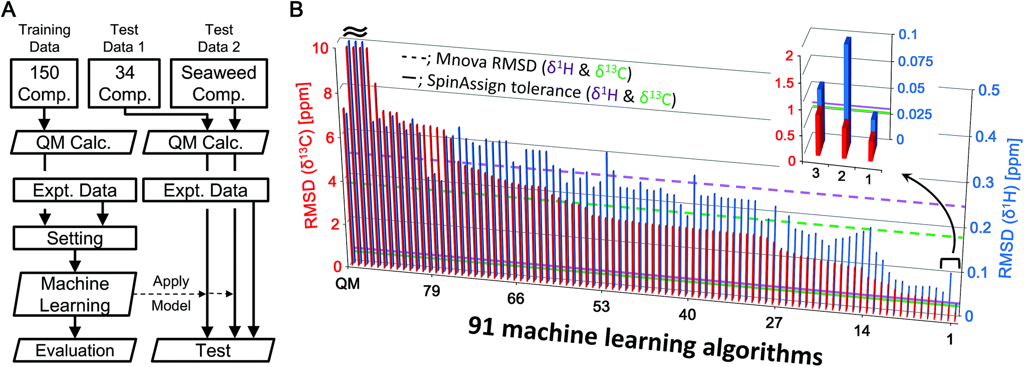 | ||
| Fig. 1 (A) Simple analytical flowchart from data collection to the evaluation of predictive modeling and testing of the predictive model using an external dataset (see the text and Fig. S1† for details). (B) Screening of 91 MLs for exploring the best predictive model. RMSDs between experimental and predicted δ1H (blue) and δ13C (red) CSs of 150 compounds as a training dataset calculated by 91 ML algorithms. These RMSDs indicate learning errors. The RMSD bars are sorted by order of accuracy of the models for δ13C. The top 3 predictive models are expanded. The left-most bar is the result from uncorrected QM. Dotted lines show the RMSD (δ1H = 0.2442 ppm, δ13C = 3.7513 ppm) of predicted CSs of 150 compounds calculated by Mnova, and solid lines show the recommended tolerances (δ1H = 0.03 ppm, δ13C = 0.53 ppm) for assignment from the SpinAssign tool. | ||
Next, predictive models for the correction of theoretical CSs that were calculated quantum chemically with B3LYP/6-311++G** (QM′) were created by the 91 ML algorithms. In this case, however, the results were almost the same for the different basis sets (Fig. S3†). On the one hand, predictive models with higher accuracy would be expected if high calculation levels such as coupled cluster singles and doubles (CCSD) were used.20 On the other hand, large calculation costs and long calculation times are associated with high calculation levels and big basis sets. As a result, the calculation level of B3LYP/6-31G* was considered to be a practical choice.
Over-learning and/or over-fitting can be a problem in predictive modeling using ML, which requires high generalization ability. This study evaluated the generalization ability of a predictive model from statistics with optimization of hyperparameters by using a grid search cross-validation (CV) algorithm to solve this problem (Table S1†). Moreover, statistical errors were evaluated by 10-fold CV (90% learning set, 10% validation set) using all combinations of each hyperparameter, and suitable predictive models with the lowest RMSD were extracted. The average RMSDs after 10-fold CV of 91 MLs are shown in Fig. S4 and S5.† In the case of the best ML algorithm xgbLinear for δ1H prediction, hyperparameters were converged (Fig. S6A†). The absolute median errors and absolute mean errors of 10 validation sets showed that the predictive performance improved significantly as compared with prediction using only QM (Fig. S6B and C†). CSs of 50% of all validation sets could be predicted within ∼0.04 ppm, and CSs of 75% of all validation sets could be predicted within ∼0.1 ppm. Also, in the case of δ13C prediction, the absolute median errors and absolute mean errors of 10 validation sets showed that the predictive performance improved significantly as compared with prediction using only QM (Fig. S7B and C†). CSs of 50% of all validation sets could be predicted within ∼0.7 ppm, and CSs of 75% of all validation sets could be predicted within ∼2.1 ppm. These results suggested that predictive modeling with both high generalization ability and high prediction accuracy was possible. On the other hand, the convergence of hyperparameters was considered insufficient (Fig. S7A†). So, the range of errors might be reduced by tuning the hyperparameters in more detail. The remaining 25% of all validation sets for δ1H prediction was predicted to be 0.1–0.94 ppm, whereas the remaining 25% of all validation sets for δ13C prediction was predicted to be 2.1–14.3 ppm. The insufficient number of structural patterns for learning may have led to this problem. Furthermore, other important factors for prediction, in addition to the explanatory variables used in this study, may be necessary. Thus, it is expected that predictive performance will improve by additional learning and the inclusion of other factors.
The Jaccard coefficient was calculated as a measure of similarity to explore what type of ML algorithm was effective as a predictor. As shown in the similarity matrix in Fig. S8† (where darker colors indicate similar models), some methods had high similarity to others. Many low Jaccard coefficients were also observed, suggesting that various types of prediction models were created and tested in this study. Furthermore, network analysis based on the Jaccard coefficients was performed with the threshold value set to 0.56 for formation of the edge (Fig. S9†). Some methods formed clusters, and the clustered methods were mostly found to have similar prediction accuracy. Notably the xgbLinear algorithm, which had the highest prediction accuracy, did not cluster with any of the other methods. In the caret library (https://topepo.github.io/caret/), the xgbLinear algorithm has the characteristic tags of “Classification,” “Regression,” “Boosting,” “Ensemble Model,” “Implicit Feature Selection,” “L1 Regularization Models,” “L2 Regularization Models,” “Linear Classifier Models,” and “Linear Regression Models”. Further improvement of prediction accuracy would be expected by developing methods of this type.
Comparison with other CS predictive methods
CSs of 34 compounds which did not include learning and k-fold validation (training) datasets of ML were used for testing the new predictive model and evaluating the predictive performance compared to other CS predictive methods. Detailed comparison between our method and existing prediction methods showed that, for the reference QM method, the RMSDs between experimental and predicted CSs were 0.3136 ppm for δ1H and 7.4477 ppm for δ13C (Fig. 2A and B). The Mnova algorithm had RMSDs of 0.2271 ppm for δ1H and 3.7600 ppm for δ13C (Fig. 2C and D). This predictive performance is excellent among existing empirical predictive methods such as NMRShiftDB. With the best ML algorithm, xgbLinear, the RMSDs were 0.2177 ppm for δ1H and 3.3261 ppm for δ13C (Fig. 2E and F). No significant error due to overfitting was observed here, and the new predictive method showed higher accuracy of CS predictions than only QM or ML methods. In particular, a high correction effect was observed in the low magnetic field side. Further detailed comparison showed that our method based on xgbLinear greatly improved prediction accuracy relative to existing methods (Fig. S10 and S11†). For Spartan software (QM2) and NMRShiftDB, the RMSDs were 0.3501 ppm (QM2) and 0.3329 ppm (NMRShiftDB) for δ1H, and 5.0681 ppm (QM2) and 4.5703 ppm (NMRShiftDB) for δ13C. For the Spartan software, for example, theoretical CSs were corrected based on the Boltzmann distribution, which led to RMSDs that were better than those from uncorrected QM′ (QM calculation with B3LYP/6-311++G**) but worse on average than those from ML algorithms. Among other methods, the NMRShiftDB web tool showed the worst accuracy for δ1H, although the ML-based NMRShiftDB algorithm23 can be expected to improve in the future. Predictive performance was ranked in the order QM′+ML > QM + ML > Mnova > QM > NMRShiftDB > QM2 > QM′ for δ1H; and QM + ML > QM′+ML > Mnova > NMRShiftDB > QM2 > QM′ > QM for δ13C. There were no significant differences in RMSDs between the two QM methods tested in this study, and thus the one with lower calculation costs would be preferable.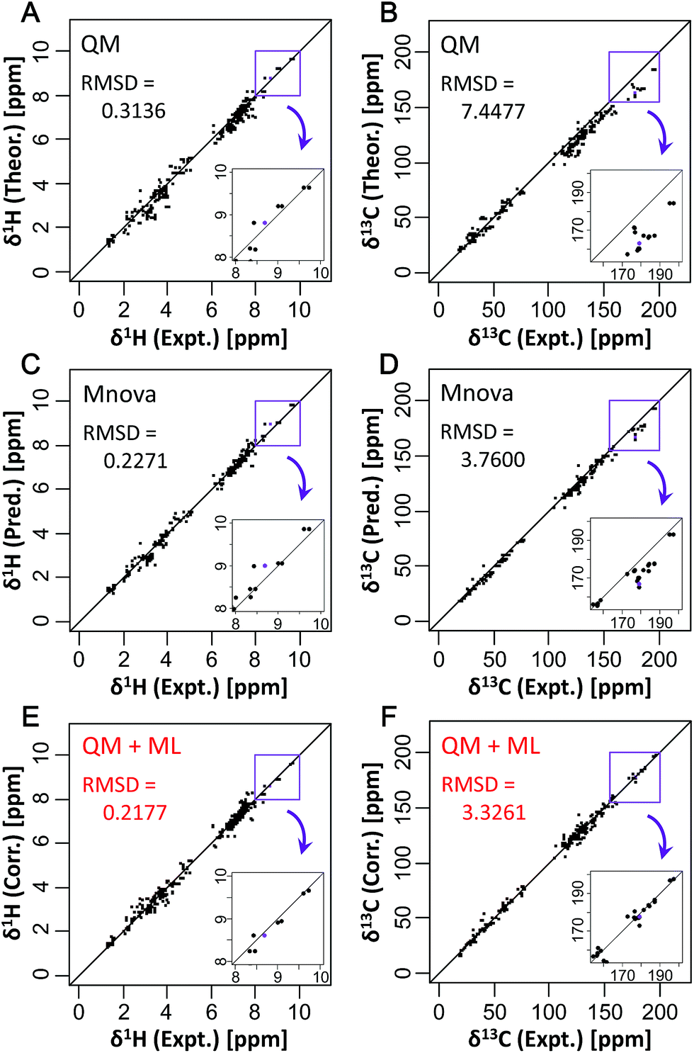 | ||
| Fig. 2 Comparison of existing predictive methods based on (A and B) quantum chemistry and (C and D) a data-driven approach with (E and F) this study's method. Experimental CSs were compared with the calculated (A, C, and E) δ1H and (B, D, and F) δ13C of 34 compounds in D2O and MeOD solvent as a test dataset. In total, 402 CSs for δ1H and 376 CSs for δ13C were plotted. Purple dots show quinolinate; the low magnetic field side around its CS is expanded in the insets. | ||
Fig. 2 shows that a remarkable correction effect was obtained with the proton and carbon of methine, and quaternary carbons such as those in carboxyl groups by the predictive approach described in this study. Moreover, we evaluated in detail the degree of improvement in prediction accuracy for different kinds of partial structures (Fig. S12†). In the case of a benzene ring containing a hydroxyl group such as 3,4-dihydroxybenzoate, both δ1H and δ13C were predicted with high accuracy. Compared with only the QM method, the prediction accuracy of the carbon atoms of the compound with a benzene ring containing nitrogen such as tryptamine was markedly improved. Also, the prediction accuracy of methylene in tryptamine for δ13C was better than that of methine in the benzene ring. However, the prediction accuracy of some δ1H had declined compared with only the QM method. For example, in the case of N-acetyl-DL-cysteine, the error of predicted δ1H near sulfur became larger than that before correction. This seemed to be due to insufficient learning for sulfur-containing compounds in the training set, i.e., there were very few compounds containing sulfur in the training set. In this manner, we found that non-existent or an insufficient number of partial structures in the training set might cause lower prediction accuracy of compounds.
To focus on the best performance of the predictive approach, only CSs of partial structures that were well learned in the training set were compared (Fig. 3, S13 and S14†). The best ML algorithm, xgbLinear, provided a highly accurate prediction for CSs of 34 compounds (Fig. 3E and F). Compared with only the QM method, the predictive errors of the QM + ML method were about 1/3 for δ1H and about 1/8 for δ13C. Also, compared with only the ML method (Mnova), the predictive errors of the QM + ML method were about 1/2 for δ1H and about 1/4 for δ13C. These results indicated that the prediction accuracy had been greatly improved compared with conventional methods. With the Mnova software, a relatively high prediction performance was obtained in various structures because the predictive model was constructed from 1.1 million CSs of 90![[thin space (1/6-em)]](https://www.rsc.org/images/entities/char_2009.gif) 000 structures (https://www.modgraph.co.uk/). Nevertheless, our developed predictive approach showed the best performance even with less training data compared to only the ML method including the Mnova software. Thus, the predictive approach described here will be able to attain more accurate and robust predictions when the predictive model is constructed from a large number of CSs of diverse structures. For this reason, we are planning to increase the number of datasets for comprehensively learning partial structures and create prediction models that will enable us to perform very accurate predictions for CSs of various structures in the future.
000 structures (https://www.modgraph.co.uk/). Nevertheless, our developed predictive approach showed the best performance even with less training data compared to only the ML method including the Mnova software. Thus, the predictive approach described here will be able to attain more accurate and robust predictions when the predictive model is constructed from a large number of CSs of diverse structures. For this reason, we are planning to increase the number of datasets for comprehensively learning partial structures and create prediction models that will enable us to perform very accurate predictions for CSs of various structures in the future.
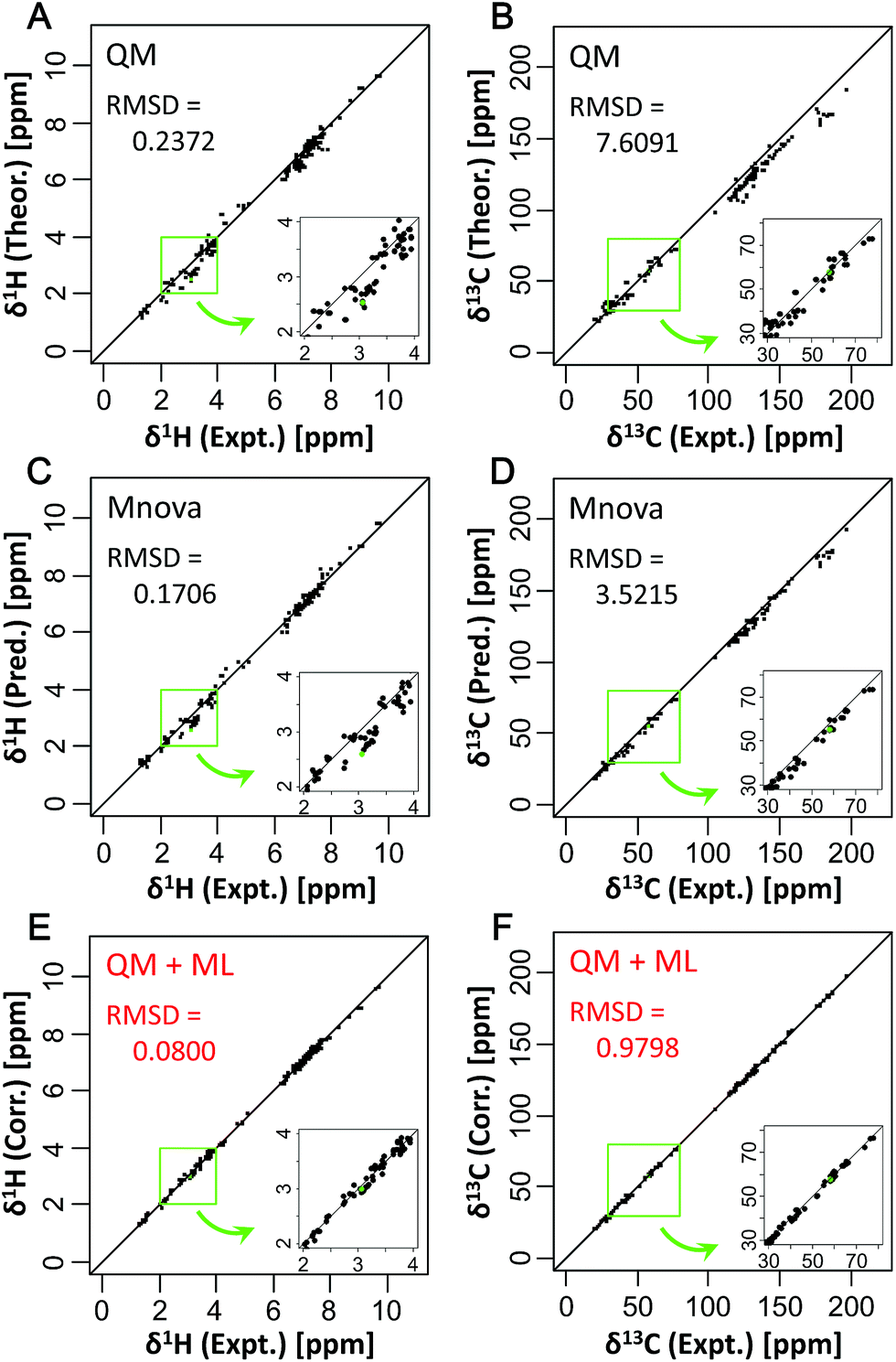 | ||
| Fig. 3 Comparison of existing predictive methods based on (A and B) quantum chemistry and (C and D) a data-driven approach with (E and F) this study's method. Experimental CSs were compared with the calculated (A, C, and E) δ1H and (B, D, and F) δ13C of 34 compounds in D2O and MeOD solvent as a test dataset. In total, 256 CSs in 402 CSs for δ1H and 216 CSs in 376 CSs for δ13C in the test dataset were plotted. Green dots show triethanolamine; the high magnetic field side around its CS is expanded in the insets. | ||
Importance of the scaling factor
In ML computation, identifying the explanatory variables (i.e., the types of data in the dataset that affect the results) is essential. For δ1H, interactions with nitrogen and carbon atoms of a 2–3 bond neighbor were the most important factors (Fig. 4A and S15A†). Thus, the interaction between hydrogen and nitrogen is considered to affect the large error. For δ13C, interactions with directly bound oxygen, carbon, and hydrogen were the most important factors (Fig. 4B and S15B†). For both δ1H and δ13C, not only the magnitude of CSs but also shielding constants were highly important factors. In the correction of both δ1H and δ13C, hydrogen–phosphorus, hydrogen–sulfur, carbon–phosphorus, and carbon–sulfur interactions had low importance. Collectively, these results indicate that subtle errors in three-dimensional structures affect the error of theoretical CSs.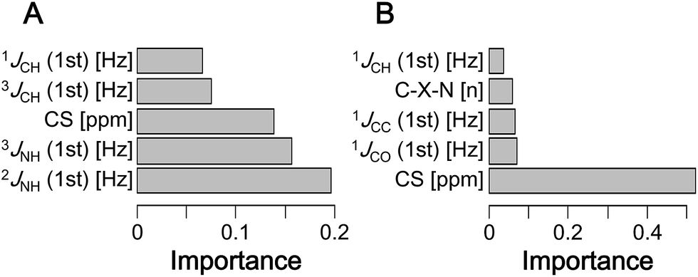 | ||
| Fig. 4 The top 5 most important explanatory variables in the predictive model with the lowest RMSD (xgbLinear) for (A) δ1H and (B) δ13C. | ||
Applying the predictive model to the assignment of metabolites
Finally, the utility of the approach was tested by applying the predictive model to the assignment of metabolites in a biological sample. For this, we used the experimental CSs of 18 metabolites in seaweed from our previous report,18 and uncorrected and corrected theoretical CSs determined in the present study were compared (Fig. 5 and S16†). The results showed that the RMSDs of the uncorrected QM method were 0.3010 ppm for δ1H and 6.8058 ppm for δ13C, while the RMSDs of the corrected QM (QM + ML) method were 0.2255 ppm for δ1H and 2.9806 ppm for δ13C. Thus, the CSs predicted by the corrected QM method were more accurate than those predicted by the uncorrected QM method. The RMSDs of each metabolite are shown in Table S2.† On the other hand, there were metabolites whose prediction accuracy declined. This decline probably occurred because the training dataset lacked data similar to those of these metabolites, and accuracy might be improved by enhancing the explanatory variables. These results suggest that the new approach can improve the performance of signal assignment of metabolites, as discussed in more detail in the ESI.† | ||
| Fig. 5 Experimental signals compared with the calculated CSs of metabolites in the C. brachypus extract by QM (×) and QM + ML (*) methods. The CSs of 16 metabolites are indicated by colored symbols (Cit, citrulline; Ala, alanine; Arg, arginine; Asp, aspartic acid; Glu, glutamic acid; Leu, leucine; Thr, threonine; 3-PGA, 3-phosphoglyceric acid; AA, acetic acid; MMA, methylmalonic acid; SA, succinate; α-Glc, α-glucose; β-Glc, β-glucose; β-GlcA, β-glucuronate; MeOH, methanol; and TMA, trimethylamine). The square indicates the RMSD (δ1H = 0.2442 ppm, δ13C = 3.7513 ppm) of predicted CSs of the 150 compounds calculated by Mnova prediction and the recommended tolerances (δ1H = 0.03 ppm, δ13C = 0.53 ppm) for assignment from the SpinAssign tool. | ||
ML approaches such as neural networks have penetrated many fields including physicochemistry,27 as shown in this study. Recently, in the field of X-ray analysis, the three-dimensional structure of metallic nanoparticles was solved by supervised machine learning (SML) based on neural networks using experimental X-ray absorption near-edge structure (XANES) spectroscopy.28 This approach can extract chemical information from experimental data or data calculated by ML, and is similar to the approach described in the present study. Jinnouchi and Asahi have also predicted the catalytic activity of nanoparticles by a DFT-aided ML algorithm.29 Their ML and DFT approach can reveal the relationship between the chemical structure and physical properties. In the future, it is likely that a similar predictive approach for chemical properties will be developed by using chemical data such as CSs and spin–spin coupling detected by NMR.
Conclusions
In this study, an advanced CS prediction model was developed by combining a QM method and an ML algorithm, and was shown to predict CSs with high accuracy as compared with existing empirical and non-empirical predictive tools. Furthermore, the utility of the model was tested by applying it to assignments of a metabolic mixture from seaweed. Thus, this study has demonstrated that the CS predictive method will be a powerful tool for the annotation and assignment of many previously unassigned signals. Its accuracy can be further enhanced by increasing the number of training datasets and explanatory variables. Based on QM and ML, the CS predictive method offers an alternative way to assign NMR signals that were previously not assigned due to difficulty in obtaining standards or experimental values, and/or the presence of metabolic “dark matter”.1 It will open up a new avenue to the assignment and annotation of metabolites in non-targeted analyses and metabolomics studies. In addition, the CS predictive method offers support to existing CS databases, leading to the development and provision of useful annotation tools on the web. In the future, a CS database based on this approach without the need for experimentation may be a powerful tool for assignment of unknown metabolites.Experimental
Structures
The analytical flow chart is summarized in Fig. 1A, and the details are provided in Fig. S1† and here. Three-dimensional structures of 150 small molecules for the training dataset (Table S3†) and 34 small molecules for the test dataset (Table S4†) were obtained from PubChem (https://pubchem.ncbi.nlm.nih.gov/). NMR spectra of these compounds in D2O and MeOD solvent are registered in an archive of the SpinAssign tool (https://dmar.riken.jp/spinassign/),12 which was developed in our laboratory. These compounds formed the training dataset used to create a CS predictive model that can link theoretical and calculated CSs.Quantum chemical calculation and other predictions
Molecular optimization, theoretical CSs, and spin–spin coupling constants were calculated quantum chemically for the 150 compounds for the training dataset and 34 compounds for the test dataset by using the Gaussian 09 program (https://gaussian.com/) installed in the HOKUSAI supercomputer at RIKEN. The calculations were performed at the B3LYP/6-31G*//GIAO/B3LYP/6-31G* and B3LYP/6-311++G**//GIAO/B3LYP/6-311++G** levels with the polarizable continuum model (PCM) method, which was used to consider solvent effects on the solute. All structures in this study were calculated by the PCM method using water and methanol models. In addition, Spartan'14 software (https://www.wavefun.com/), the NMRShiftDB webtool (https://nmrshiftdb.nmr.uni-koeln.de/), and Mnova software (https://mestrelab.com/) were used to calculate predicted CSs in order to compare the performance of the new approach with existing methods. In Spartan'14 software, theoretical CSs were calculated at the EDF2/6-31G* level, and were corrected with the weighted average based on Boltzmann distribution after conformational analysis. In the predictive function of the NMRShiftDB webtool, three spheres were set as the predictive configuration.22,23 In Mnova software, the Mnova ‘Best’ prediction method, which adopts a ML algorithm, was chosen.Experimental data
In total, 150 standard substances for the training dataset and 34 standard substances for the test dataset were prepared in two solvents (KPi/D2O and MeOD, pH = 7.0). NMR spectra of the standard substances were acquired at 298 K on a 500, 600, or 700 MHz Bruker Biospin NMR instrument. All data were collected under a unified global standard condition. Experimental CSs for each fragment of the 150 compounds in KPi/D2O and MeOD solvent were assigned by using the SpinAssign tool, BMRB,7,8 and HMDB9 as NMR databases; in addition, the Mnova software was used to assist in assignment.Setting the training data
The objective variable used by the ML algorithm as an index for prediction was the difference (Diff.) between the experimental and theoretical CSs:| Diff. = CS(Expt.) − CS(Theor.) |
The theoretical CS, the spin–spin coupling constant, the number and atomic species of chemical bond neighbors, the number of attached protons, solvent type, aromatic type, and pyranose type were collected as explanatory variables for predicting the objective variable (Table S5 and S6†). This dataset was automatically configured and extracted from the result files of QM calculation by using a Java program. The number of ML datasets was 1277 for δ1H and 1078 for δ13C for the 150 compounds in D2O and MeOD solvents.
Machine learning for predictive modeling
The conditions for creating a good predictive model vary with algorithm type, hyperparameters, and dataset. Therefore, it is necessary to use various ML algorithms to create an optimal prediction model. In this study, 91 ML algorithms were explored to identify a useful algorithm for creating the CS predictive model (Table S7†). These 91 ML algorithms were taken from the caret library30 of R-3.4.1 software (https://www.r-project.org/) and Microsoft R Open-3.3.3 software (https://mran.microsoft.com/open/) and used to calculate the scaling factor (SF) and the importance of explanatory variables. The predicted difference (Diff.) equals the SF.| SF = predicted diff. |
The predicted CS was calculated by adding the SF to the theoretical CS determined by the QM method.
| Predicted (corrected) CS = CS(Theor.) + SF |
Tuning the hyperparameters and evaluation
Configuration of the hyperparameters of ML is necessary to generate a suitable predictive model. In general, the hyperparameters provided in ML programs are set to default variables. However, optimizing the hyperparameters is necessary because default variables are not always appropriate. On the other hand, manually optimizing the hyperparameters of many ML algorithms manually is labor-intensive. Moreover, at present, the problem of over-fitting by over-learning must also be avoided. So, hyperparameters of the 91 ML algorithms explored in this study were tuned automatically by a grid search CV approach in the caret library of R software.30 The grid search approach tries all combinations of candidate variables of a specified hyperparameter.31 Moreover, the most suitable combination can be determined by an index such as RMSD, which is calculated by CV. This approach is defined as the grid function in each ML program of the caret library for a comprehensive search.30 The exploratory range is decided automatically depending on the dataset, type of hyperparameter, and ML algorithm. Here, hyperparameter combinations with up to 3 grids were tried, and the most suitable combinations were identified (Table S1†). For the grid search, 10-fold CV (10% = validation set, 90% = learning set) was used to evaluate over-learning and generalization performance. For δ1H prediction, 128 CSs were used as the validation set, and 1149 CSs were used as the learning set. For δ13C prediction, 108 CSs were used as the validation set, and 970 CSs were used as the learning set. The validation and learning sets were chosen randomly and chosen not to overlap with the train function in the caret library. The final predictive model and hyperparameters were decided from the lowest RMSD identified by the 3-grid search 10-fold CV. We used the grid search approach because it can simplify screening of hyperparameters and can be implemented in various ML algorithms. However, further hyperparameter optimization might be achieved by manual fine-tuning or using other automatic parameter search methods, such as randomized search,31 genetic algorithms,32 and so on.Example data and programs for generating datasets for ML from experimental/theoretical (log files of the Gaussian 09 program) data and the 91 MLs with the grid search CV approach used in this study are available on our website (https://dmar.riken.jp/Rscripts/).
Comparison of the performance among MLs
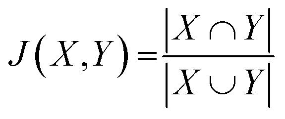
Each predicted CS was evaluated by plotting the RMSD from the experimental CS. The predictive performance of the new method was evaluated by comparison with existing predictive methods. To explore the relationship between the predictive performance and ML algorithm type, the Jaccard coefficient (J) was calculated as follows:where X and Y are sets of two ML algorithms, and each set consists of 59 elements. The elements are the ML algorithm types defined in the caret library (Table S8†).
Test of the QM + ML predictive model and comparison with other predictions using an external test dataset
The predictive model was tested and compared with other prediction methods using two datasets for evaluation of over-fitting and general performance. One contained 34 compounds which were randomly chosen to verify the accuracy of predictions as a separate and unseen test dataset because a sufficiently large dataset comprising at least 20% of the data is the required minimum to guard against over-fitting. The utility of the new predictive model was also tested by applying it to the assignment of another dataset: in this case, 18 metabolites in a seaweed (C. brachypus) extract that we previously characterized.18Conflicts of interest
There are no conflicts to declare.Acknowledgements
The authors thank T. Matsumoto and A. Tei (RIKEN) for their support and encouragement during this study. The RIKEN Advanced Center for Computing and Communication also provided use of a supercomputer, HOKUSAI. This research was partially supported by MAFF.Notes and references
- J. L. Markley, R. Brüschweiler, A. S. Edison, H. R. Eghbalnia, R. Powers, D. Raftery and D. S. Wishart, Curr. Opin. Biotechnol., 2017, 43, 34–40 CrossRef PubMed
.
- M. P. Williamson and C. J. Craven, J. Biomol. NMR, 2009, 43, 131–143 CrossRef PubMed
- S. Lee, H. Wen, Y. J. An, J. W. Cha, Y. J. Ko, S. G. Hyberts and S. Park, Anal. Chem., 2017, 89, 1078–1085 CrossRef PubMed
- P. Soininen, A. J. Kangas, P. Würtz, T. Suna and M. Ala-Korpela, Circ.: Cardiovasc. Genet., 2015, 8, 192–206 Search PubMed
- D. Jeannerat, Magn. Reson. Chem., 2017, 55, 7–14 CrossRef PubMed
- T. Komatsu and J. Kikuchi, J. Phys. Chem. Lett., 2013, 4, 2279–2283 CrossRef
- E. L. Ulrich, H. Akutsu, J. F. Doreleijers, Y. Harano, Y. E. Ioannidis, J. Lin, M. Livny, S. Mading, D. Maziuk and Z. Miller, Nucleic Acids Res., 2008, 36, 402–408 CrossRef PubMed
- J. L. Markley, E. L. Ulrich, H. M. Berman, K. Henrick, H. Nakamura and H. Akutsu, J. Biomol. NMR, 2008, 40, 153–155 CrossRef PubMed
- D. S. Wishart, T. Jewison, A. C. Guo, M. Wilson, C. Knox, Y. Liu, Y. Djoumbou, R. Mandal, F. Aziat, E. Dong, S. Bouatra, I. Sinelnikov, D. Arndt, J. Xia, P. Liu, F. Yallou, T. Bjorndahl, R. Perez-Pineiro, R. Eisner, F. Allen, V. Neveu, R. Greiner and A. Scalbert, Nucleic Acids Res., 2013, 41, 801–807 CrossRef PubMed
- Q. Cui, I. A. Lewis, A. D. Hegeman, M. E. Anderson, J. Li, C. F. Schulte, W. M. Westler, H. R. Eghbalnia, M. R. Sussman and J. L. Markley, Nat. Biotechnol., 2008, 26, 162–164 CrossRef PubMed
- K. Bingol, D. W. Li, B. Zhang and R. Brüschweiler, Anal. Chem., 2016, 88, 12411–12418 CrossRef PubMed
- E. Chikayama, Y. Sekiyama, M. Okamoto, Y. Nakanishi, Y. Tsuboi, K. Akiyama, K. Saito, K. Shinozaki and J. Kikuchi, Anal. Chem., 2010, 82, 1653–1658 CrossRef PubMed
- J. Kikuchi, Y. Tsuboi, K. Komatsu, M. Gomi, E. Chikayama and Y. Date, Anal. Chem., 2016, 88, 659–665 CrossRef PubMed
- E. Chikayama, Y. Shimbo, K. Komatsu and J. Kikuchi, J. Phys. Chem. B, 2016, 120, 3479–3487 CrossRef PubMed
- M. W. Lodewyk, M. R. Siebert and D. J. Tantillo, Chem. Rev., 2012, 112, 1839–1862 CrossRef PubMed
- D. Muri, C. Corminboeuf, E. M. Carreira and D. Jeannerat, Magn. Reson. Chem., 2009, 47, 909–916 CrossRef PubMed
- T. Komatsu, R. Ohishi, A. Shino and J. Kikuchi, Angew. Chem., Int. Ed., 2016, 55, 6000–6003 CrossRef PubMed
- K. Ito, Y. Tsutsumi, Y. Date and J. Kikuchi, ACS Chem. Biol., 2016, 11, 1030–1038 CrossRef PubMed
- T. Misawa, T. Komatsu, Y. Date and J. Kikuchi, Chem. Commun., 2016, 52, 2964–2967 RSC
- R. Faber and S. P. A. Sauer, AIP Conf. Proc., 2015, 1702, 090035 CrossRef
- F. Hoffmann, D. W. Li, D. Sebastiani and R. Brüschweiler, J. Phys. Chem. A, 2017, 121, 3071–3078 CrossRef PubMed
- C. Steinbeck and S. Kuhn, Phytochemistry, 2004, 65, 2711–2717 CrossRef PubMed
- S. Kuhn, B. Egert, S. Neumann and C. Steinbeck, BMC Bioinf., 2008, 9, 400 CrossRef PubMed
- S. Grimme, C. Bannwarth, S. Dohm, A. Hansen, J. Pisarek, P. Pracht, J. Seibert and F. Neese, Angew. Chem., Int. Ed., 2017, 56, 14763–14769 CrossRef PubMed
- J. Lehtivarjo, M. Niemitz and S. P. Korhonen, J. Chem. Inf. Model., 2014, 54, 810–817 CrossRef PubMed
- T. Chen and C. Guestrin, ACM, 2016, 785–794 Search PubMed
- W. F. Schneider and H. Guo, J. Phys. Chem. Lett., 2018, 9, 569 CrossRef PubMed
- J. Timoshenko, D. Lu, Y. Lin and A. I. Frenkel, J. Phys. Chem. Lett., 2017, 8, 5091–5098 CrossRef PubMed
- R. Jinnouchi and R. Asahi, J. Phys. Chem. Lett., 2017, 8, 4279–4283 CrossRef PubMed
- M. Kuhn, J. Stat. Softw., 2008, 28, 1–26 Search PubMed
- J. Bergstra and Y. Bengio, J. Mach. Learn. Res., 2012, 13, 281–305 Search PubMed
- M. Zhao, C. Fu, L. Ji, K. Tang and M. Zhou, Expert Syst. Appl., 2011, 38, 5197–5204 CrossRef
Footnote |
| † Electronic supplementary information (ESI) available. See DOI: 10.1039/c8sc03628d |
| This journal is © The Royal Society of Chemistry 2018 |