The crucial role of a spacer material on the efficiency of charge transfer processes in organic donor–acceptor junction solar cells

Abstract

Organic photovoltaic donor–acceptor junction devices composed of π-conjugated polymer electron donors (D) and fullerene electron acceptors (A) show greatly increased performance when a spacer material is inserted between the two layers (W. Y. Nie, G. Gupta, B. K. Crone, F. L. Liu, D. L. Smith, P. P. Ruden, C. Y. Kuo, H. Tsai, H. L. Wang, H. Li, S. Tretiak and A. D. Mohite, Adv. Sci., 2015, 2, 1500024.). For instance, experimental results reveal significant improvement of photocurrent when a terthiophene oligomer derivative is inserted in between π-conjugated poly(3-hexylthiophene-2,5-diyl) (P3HT) donor and C₆₀ acceptor. These results indicate favorable charge separation dynamics, which is addressed by our present joint theoretical/experimental study establishing the beneficial alignment of electronic levels due to the specific morphology of the material. Namely, based on the experimental data we have constructed extended structural interface models containing C₆₀ fullerenes and P3HT separated by aligned oligomer chains. Our time-dependent density functional theory (TD-DFT) calculations based on a long-range corrected functional, allowed us to address the energetics of essential electronic states and analyze them in terms of charge transfer (CT) character. Specifically, the simulations reveal the electronic spectra composed of a ladder of excited states evolving excitation toward spatial charge separation: an initial excitonic excitation at P3HT decomposes into charges by sequentially relaxing through bands of C₆₀-centric, oligomer → C₆₀ and P3HT → C₆₀ CT states. Our modeling exposes a critical role of dielectric environment effects and electronic couplings in the self-assembled spacer oligomer layer on the energetics of critical CT states leading to a reduced back-electron transfer, preventing recombination losses, and thus rationalizes physical processes underpinning experimental observations.

---

1. Introduction

The interfaces of organic photovoltaic bulk heterojunction (BHJ) donor (D)/acceptor (A) devices between π-conjugated electron donor polymers and electron acceptors, such as fullerenes, are of fundamental importance for understanding organic photovoltaic processes and for improving their efficiency.^1–3 These interfaces control the dissociation of excitons and generation of charge transfer (CT) states. The conversion of light into electricity in a BHJ photovoltaic device is accomplished by a four-step process: (i) light absorption by bright π → π* transition of the organic conjugated polymer and generation of excitons, (ii) diffusion of the excitons through the bulk polymer and segregation to the interface, (iii) dissociation of the excitons at afore-mentioned heterojunctions and creation of CT states, and (iv) charge separation and collection at contacts.^1,4 The actual processes occurring in the BHJ material are significantly more complex because of the heterogeneous distribution of donor and acceptor in the BHJ material, a broad variety of structural defects and conformations, the large number of internal degrees of freedom of the polymer chains, and the complicated manifold of electronic states.^5–7 Therefore, finessing the mechanism of ultrafast and loss-less free charge generation in BHJ devices via intercede design is still a very active research area.^8–12

While traditional organic photovoltaic (OPV) BHJ devices involve only a pair of materials, i.e., electron donor and acceptor complexes, recent experimental work¹³ has employed a new strategy of using a third material acting as a spacer between the donor and acceptor regions,^14,15 which mitigates the electron–hole recombination rate (i.e. the backward charge transfer processes) but without affecting the efficiency of charge separation (i.e., forward electron transfer). In particular, these studies in a simple bi-layer device have shown a large increase in both the photocurrent (up to 800%) and open circuit voltage (V_OC) when a spacer material such as a terthiophene-derivative (O3) is added between the donor, a poly(3-hexylthiophene-2,5-diyl) (P3HT), and a fullerene (C₆₀) acceptor. Subsequently, in the BHJ device a significant increase in the power conversion efficiency (PCE) from 4% to greater than 7% was observed.¹³ These experimental findings followed the hypothesis of a “fast energy transfer of the exciton from the donor across O3 to the acceptor and the back cascading of the hole to the donor” due to a favorable alignment of the corresponding energy levels. Such arrangement ensures that the spacer material is also physically separating the donor and acceptor interface thus working to mitigate the CT recombination rate.

Quantum-chemical modeling of these materials can provide important atomistic insights into the nature of underlining processes and ultimately help to formulate design strategies toward optimizing the photophysical dynamics. The first important step is the determination of the energy level alignment occurring at the complex donor–acceptor interfaces. For such large systems density functional theory (DFT) and time-dependent (TD)-DFT are the most widely used techniques providing access to the ground and excited state properties, respectively, being a reasonable compromise between accuracy and numerical cost. However, in spite of the overwhelming success of DFT in ground-state computation, the correct description of charge-separated excited states is still problematic for many developed exchange–correlation functionals due to the significant delocalized nature of the density, especially for intermolecular CT states at BHJ interfaces.^16–19 A variety of strategies have been developed to correctly account for delocalized excitations. Long-range corrected functionals^20,21 in combination with optimization of the parameters determining the separation range^22–25 have been used successfully to correct several TD-DFT artifacts. In previous work,²⁶ we have shown that long-range corrected functionals of CAM-B3LYP^27,28 and ωB97XD²⁹ gave very good agreement for excitonic and CT states for thiolated oligothiophene dimers in comparison to the second-order algebraic diagrammatic construction (ADC(2)) approach. Thus, long-range corrected functionals appear to be well applicable for the calculation of electronic spectra of π-conjugated semiconductor polymers including capacity of describing both excitonic and CT states.³⁰ They are also computationally efficient so that the capability of treating large molecular aggregate systems can be well managed.

Regarding the discussed bilayer interfaces,³¹ previous calculations have shown that the bright, light absorbing π → π* transition can be located above CT states and can convert to the CT state via internal conversion processes. However, it has been concluded from TD-DFT calculations³² that dark fullerene states could be located even lower in energy and would have the possibility to quench the CT states after they have been formed. Other calculations based on the already mentioned ADC(2) method have shown a slightly different picture indicating CT states as the lowest singlet states.^31,33

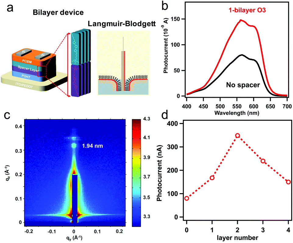
The energetic ordering of states and the stabilization of CT states obviously represents a crucial issue affecting the reduction of unwanted leaking processes. This joint experimental and computational study wants to demonstrate the specific factors affecting especially the stability of the CT states. For that purpose, the experimental P3HT/O3/C₆₀ system discussed above is being used together with our previously benchmarked TD-DFT methodology.²⁶ Even though the calculations are specific for this system, as we will show, the conclusions are quite general and can certainly be transferred to many other polar interface systems. Two structural models were employed in order to represent the donor–spacer–acceptor interface: (i) the donor P3HT polymer is connected via one spacer T3 chain to the acceptor C₆₀ (Fig. 1a, denoted as standard model) and (ii) an extended model (Fig. 1b and c) where P3HT is connected via three T3 spacer molecules to three C₆₀ electron acceptors. A spacer material, thiolated terthiophene, T3, was used which can be considered as a good approximation to O3 used in the experiments. This specific mutual arrangement of molecules underscores our experimental fabrication technique utilizing the Langmuir–Blodgett (LB) method (Fig. 2a) ensuring orthogonal orientation of the oligomer with respect to the polymer P3HT layer, as demonstrated by our X-ray measurements. Furthermore, the extended model aims to account for π-stacking effects in the oligomer, which were shown to be important for conventional, simple donor–acceptor interfaces.^34–39

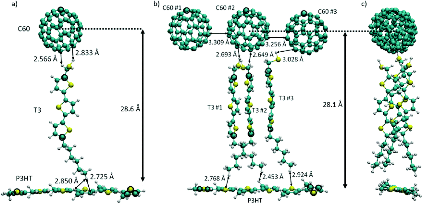Fig. 1 (a) Standard model of the molecular arrangement in the trimer. (b) Front and (c) side views of the extended model. The picture shows molecular notations, geometrical arrangement and selected nonbonding distances (Å). Atoms kept fixed during the geometry optimization are circled in black.

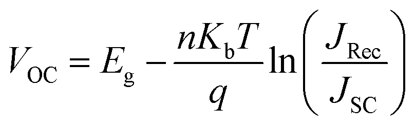
Fig. 2 (a) Scheme of bilayer device structure used in this study, the interface layer with vertical alignment was produced by Langmuir–Blodgett (LB) method illustrated on right. (b) Photocurrent measured at short circuit condition as function of illumination wavelength for bilayer device without spacer and with 1-bilayer of O3 between P3HT and C₆₀. (c) GIWAXS map for 1 bilayer of O3 deposited on P3HT by LB method. (d) Peak photocurrent at 550 nm illumination as a function of number of O3 bilayer at interface.

The article is organized as follows: section 2 describes experimental and computational methodology, section 3 presents our results, and finally section 4 summarizes our findings and conclusions.

2. Methods

2.1. Experimental

2.1.1. Bilayer solar cells fabrication. Solar cell fabrication started from the cleaning of indium tin oxide (ITO) transparent substrate with sonication bath in water, acetone and isopropyl alcohol for 15 min respectively. The hole transporting polymer poly(3,4-ethylenedioxythiophene) polystyrene sulfonate (PEDOT:PSS) solution was then coated on the cleaned ITO substrates by spin coating method. After drying, the coated substrates were transferred to an argon filled glovebox for P3HT coating. The in-stock P3HT solution (2 mg ml⁻¹ in chlorobenzene) was spin coated on the substrates at 2000 rpm for 45 s, forming a uniform, 40 nm thin film without further annealing. The coated substrates were then taken outside the glovebox for interfacial layer deposition by LB technique between air–water interfaces on a spin coated P3HT film. After LB deposition, the devices were completed by thermally evaporating C₆₀ (30 nm) for acceptor layer and electrode deposition through shadow mask.

2.1.2. Device characterization. The completed solar cells were mounted in cryostat with BNC connections from the electrodes to the instruments. The photocurrent was collected in AC mode by illuminating the device with monochromatic light while measuring the short circuit current using lock-in amplifier.

2.2. Computational details

The computational methods are based on DFT using the Perdew–Burke–Ernzerhof (PBE)⁴⁰ functional with the SV(P)⁴¹ basis for geometry optimizations, and the long-range separated density functional, CAM-B3LYP, for the calculation of excited states using two basis sets, 6-31G⁴² and 6-31G*.^43,44 Solvent effects were taken into account using the conductor-like polarizable continuum model (C-PCM).⁴⁵ Environmental effects on the electronically excited states were investigated on the basis of the linear response (LR)^46,47 and state-specific (SS)⁴⁸ approaches. Dichloromethane (dielectric constant, ε = 8.93, refractive index, n = 1.42) was chosen to act as a modestly polar environment. Geometry optimizations were performed by freezing selected atoms as shown in Fig. 1 in order to maintain the desired structure of the aggregate as deduced from experiment.

Geometry optimizations were carried out using the TURBOMOLE⁴⁹ program suite, while all TD-DFT calculations were performed with the Gaussian G09 program package.⁵⁰ The character of the electronic states has been analyzed by means of natural transition orbitals (NTOs)^51–53 and molecular electrostatic potential plots (MEP). NTOs represent the weighted contribution to each excited state transition from a hole to a particle (electron) derived from the one-electron transition density matrix. NTOs and particle/hole populations were performed with the TheoDORE program package.^54–56

For more detailed information see the ESI.†

3. Results and discussion

3.1. Experimental observations

We fabricate the bilayer device as illustrated in Fig. 2a comprised with 20 nm P3HT as donor and 40 nm of fullerene (C₆₀) as acceptor for photocurrent measurements as summarized in Fig. 2. To insert oriented O3 between the (D/A) interface, we employed the O3 with Langmuir–Blodgett (LB) method after spin coating P3HT on hole transporting material, followed by C₆₀ deposition by thermal evaporation (Fig. 2a). The obtained bilayer device was taken for photocurrent spectrum measurement in Fig. 2b. The photocurrent follows the absorption spectrum of P3HT (band gap 1.9 eV), while the magnitude of the photocurrent increase by 1.8 times from the device without spacer layer (black) to the device with 1-bilayer of O3 inserted (red). The optical band gap remains the same in both cases indicating the oligomer absorption does not contribute to the photocurrent increase. To characterize the molecular orientation of the O3 molecules at the interface, we took the LB deposited O3 molecules on P3HT thin-film for gracing incidence wide angle X-ray scattering (GIWAXS) measurement. The result in Fig. 2c clearly shows a diffraction spot along the q_z axis. The spot is located near q_z = 0.322 Å⁻¹ corresponding to a d-spacing of 19.4 Å which matches with the molecule length. In addition, the Bragg spots are parallel to the q_y axis (substrate) indicating that the O3 molecules are aligning in the out-of-plane⁵⁷ orientation by LB method (Fig. 2a) and pointing from P3HT towards C₆₀. The distance between the donor–acceptor is thus determined by the length of molecule and number of bilayers deposited. This is consistent with previous measurements of three self-assembled oligomers.^13,58 We further performed device photocurrent measurement as a function of the number of O3 bilayers as shown in Fig. 2d, we found the maximum gain in photocurrent can be obtained when inserting two bilayers of O3 molecules between D/A interface. This is suggesting that such separation between donor and acceptor materials is optimal to suppress the electron–hole recombination through CT state at the interface after a suitable thickness of spacer layer insertion. The subsequent decrease of the photocurrent is associated with the decrease of efficiency for direct CT process.

At open circuit condition, the photo-voltage value is determined by the carrier generation and recombination, following the equation:

where E_g is the effective band gap, K_b is the Boltzmann constant, T is the temperature, q is the elementary charge, J_Rec is the recombination current and J_SC is the final short circuit photocurrent density.⁵⁹ Considering a dielectric constant of 3–4 in a typical organic system, the Coulomb radius is estimated to be 16 nm,⁶⁰ and the energetic disorder further reduces this value to 4 nm, probed experimentally.¹⁰ This means that if the electron–hole pair bonded at the charge transfer states can be separated to a distance greater than the Coulomb radius, significant amount of carrier recombination can be suppressed, that reduces J_REC and increases J_SC, which ultimately reduces the voltage loss through non-radiative recombination. In fact, our experimental data in Fig. 2 show an increase in J_SC (photocurrent at short circuit condition) which is an indication of reduced recombination that will lead to increase in V_OC.

The purpose of the following electronic structure calculations is to show that such a large electron–hole separation is energetically feasible using the detailed interface models shown in Fig. 1. At this point it should be mentioned that in the single spacer level model used because of computational economy, the electron–hole pair will have a separation of only ∼3 nm.

3.2. Analysis of energy levels

The geometrical arrangement of the three components of the standard model is depicted in Fig. 1a. In this model only a single T3 layer is used because of computational efficiency. Nevertheless, as the results below will show, the major stabilization effects for charge separated states can be seen already in this case. The spacer T3 chain faces the C₆₀ unit via the thiol group with interatomic distances of 2.6–2.8 Å and P3HT via the alkane chain at distances of 2.7–2.85 Å. The distance between the center of C₆₀ and P3HT is ∼28.6 Å. In the extended model (Fig. 1b and c) three C₆₀ units are arranged horizontally with distances of around 3.3 Å. The three T3 chains are stacked (side view, Fig. 1c). Typical intermolecular distances are displayed in Fig. 1: (a) standard model of the molecular arrangement in the trimer. The Cartesian coordinates for the standard and extended model are given in the ESI.†

The calculations on the standard trimer have been used to establish the general structure of the electronic spectrum and to test the validity of the smaller 6-31G basis set for use with the significantly larger extended trimer. The scheme of the lowest excited singlet states of the isolated complex is given in Fig. 3a and b using the 6-31G* and 6-31G basis sets, respectively. The full list of the 20 excited singlet state energies Ω calculated can be found in Table S1† (6-31G basis) and Table S2 (6-31G* basis) of the ESI.† For the 6-31G* basis (Fig. 3a, isolated system), the local C₆₀ states have been calculated as well. This figure shows that in case of the calculation for the isolated system they form the lowest band of excitonic states. If this would be the true energy ordering, these states would act as a sink for conversion of CT states, which would lead to serious losses for the efficiency of the photovoltaic process. The C₆₀ states are followed by a local π–π* state on P3HT which has the largest oscillator strength, f, of all states calculated. Next appears another band of C₆₀ states followed by two closely spaced triples of CT states from P3HT → C₆₀ and T3 → C₆₀ at 3.3 and 3.4 eV, respectively. There are two more locally excited states, one on T3 and the other one on P3HT. Triples of CT states alternating between excitations from P3HT and T3 follow. This sequence is interrupted only by one local state on P3HT. Inclusion of the environment via the LR method (Fig. 3a and b and Tables S4 and S5†) does not change much in the relative ordering of states compared to the isolated system. However, the more sophisticated, but also numerically more expensive SS solvent calculations change the situation dramatically (Fig. 3a, Table S6†). With respect to the P3HT excitonic bright state, the SS approach leads to a quite dramatic stabilization of nine CT states to be located below the P3HT state. The energetic spacing between the P3HT → C₆₀ CT states and the T3 → C₆₀ CT states is rather large being about 0.6 eV. There is also a large energy gap of about 0.75 eV between the P3HT state and the following T3 → C₆₀ CT state. Thus, from this model one can already see the crucial environmental effect which significantly stabilizes the CT state relative to the others. On the other side, the environmental effect on the energetic location of the locally excited P3HT and C₆₀ states is small. As a result, the CT states are the lowest ones and the leaking of the CT states into locally excited C₆₀ states is avoided.

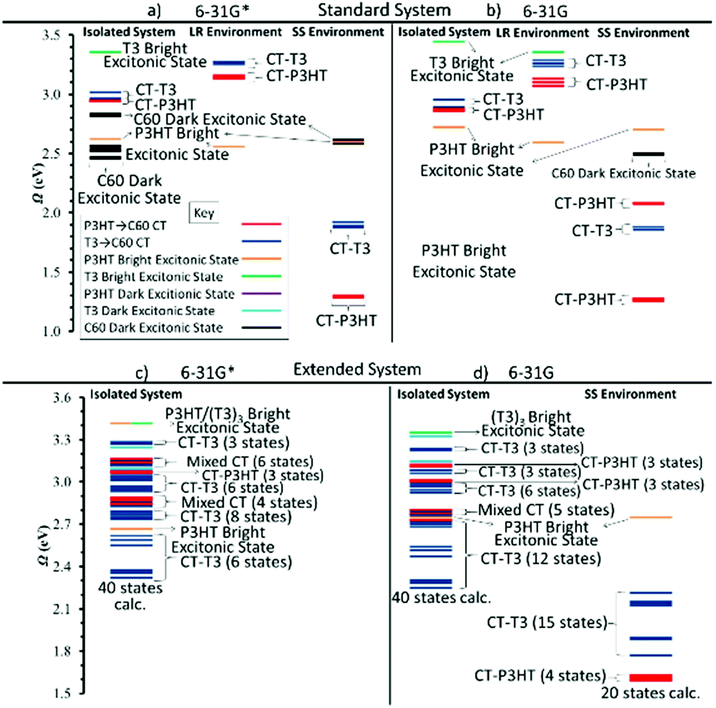Fig. 3 Excited state energies Ω of the standard P3HT–T3–C₆₀ trimer using the CAM-B3LYP method and (a) the 6-31G* and (b) the 6-31G basis sets both as isolated systems and in the LR and SS environments (for numerical data see Tables S1, S2, and S4–S8†). For the isolated system using the 6-31G* basis set (farthest left of (a)), the fifteen lowest-energy locally excited C₆₀ states have been computed also. Excited states of (c) the extended P3HT–T3–C₆₀ trimer using the 6-31G* and (d) 6-31G basis sets both as isolated systems and in the SS environment (Tables S9–S11†).

The strongly different behavior of the two solvation models is to be expected since in the LR method dynamic solvent polarization is computed from the transition density which is, however, very small as shown for the present case of charge transfer states. Consequently, the solvent effects are correspondingly small and not adequately represented by this approach in the case of charge transfer states. On the other hand, the SS approach has been developed having charge-transfer transitions in mind by representing the dynamic solvent polarization by means of the difference of the electronic densities of the initial and final states. For a more detailed discussion of this point see e.g.ref. 61. Therefore, it is concluded that the SS scheme allows for a better characterization of environmental effects on CT states and the LR approach has been presented only for comparison reasons. It will not be considered further here.

Comparison between the 6-31G* and 6-31G basis sets shows that the smaller 6-31G basis represents the energy spectrum of the standard complex very well and also that omission of the C₆₀ states by freezing respective orbitals does not affect the remaining spectrum. These findings are important for the calculations on the extended trimer where the state-specific (SS) solvent calculations are time consuming. Therefore, they have been performed only with the 6-31G basis (see below).

The extended trimer was investigated next as an extension of our standard trimer structure providing a significantly enhanced interface model (Fig. 3c and d, Tables S9–S11†). For the isolated system, the lowest bright state is located on P3HT at ∼2.65 eV, very similar to the excitation energy in the standard model. The difference to the standard model is that now several (T3)₃ → (C₆₀)₃ CT states are located below even for the isolated complex. A rich variety of states is also found above the P3HT state (Fig. 3c).

Including the SS environment using the 6-31G basis, Fig. 3d, results in significant changes with respect to the CT states, the most important one being that the P3HT CT states are lowest in energy. Below the P3HT bright excitonic state, we computed nineteen CT states: fifteen (T3)₃ → (C₆₀)₃ CT states and four P3HT → (C₆₀)₃ CT states. The (T3)₃ → (C₆₀)₃ CT states occupy a CT band of 0.44 eV, while the P3HT → (C₆₀)₃ CT states are found in a much narrower range of 0.02 eV. As has already been found for the standard model, the mentioned CT states are located significantly below the C₆₀ states (which are around 2.5 eV) and that, therefore, the former states cannot leak into C₆₀ states as soon as they are formed. In contrast to the results presented here, in TD-DFT thiophene/fullerene complexes³² locally excited C₆₀ states comprised the lowest-energy band of states. These differences are probably due to the use of the LR solvation model used in this reference. It is important to point out that the presence of any π-conjugated chromophores adds an effective dielectric medium and facilitates further stabilization of CT states even though the wavefunction is not directly delocalized into these molecules. To illustrate this trait, we removed the spacer and calculated only the C₆₀/P3HT system. Table 1 records the calculated energies of the lowest P3HT → C₆₀ CT states. In the P3HT–T3–C₆₀ system, the solvent stabilization is 1.62 eV, but in the P3HT–C₆₀ system only 0.42 eV. This comparison shows the strong sensitivity of the electrostatic interaction in the charge separated systems which are better stabilized by the environment in the case where the charge separation is more pronounced due to the spacer in between.

Table 1 Stabilization energy of the lowest P3HT → C₆₀ CT state of P3HT–T3–C₆₀ and P3HT–C₆₀ system calculated in the isolated system and the state-specific (SS) environment

	P3HT–T3–C60	P3HT–C60
Isolated system	2.91	2.20
SS environment	1.29	1.78
ΔE (eV)	1.62	0.42

---

3.3. Characterization of electronic states

The properties of the different types of electronic states are characterized in Fig. 4 by means of two descriptors. The first one is represented by the most important NTO's of typical electronic transitions of the systems calculated in the SS environment (Fig. 4). All transitions are well represented with one hole/particle pair as the corresponding weights are above 0.9 e. As discussed above, the lowest excited singlet state band has P3HT → (C₆₀)₃ CT character. This can be nicely seen from the NTO picture of Fig. 4a and b, which shows, respectively, the hole density in P3HT and the particle density in the central C₆₀ unit. These two densities are well separated with essentially no overlap between the two systems. As a second descriptor, the molecular electrostatic potential (MEP) plot displayed in Fig. 4c shows that the P3HT unit has a strongly positive potential which extends significantly into the (T3)₃ moiety. The electrostatic potential of the middle C₆₀ molecule of the (C₆₀)₃ unit is strongly negative in agreement with the location of the particle NTO in Fig. 4b. The other two C₆₀ molecules are slightly negative as well. Overall, the MEP plots give a stronger delocalized picture of the CT process in comparison to the NTOs, since the localized CT density affects much larger regions via Coulomb interactions.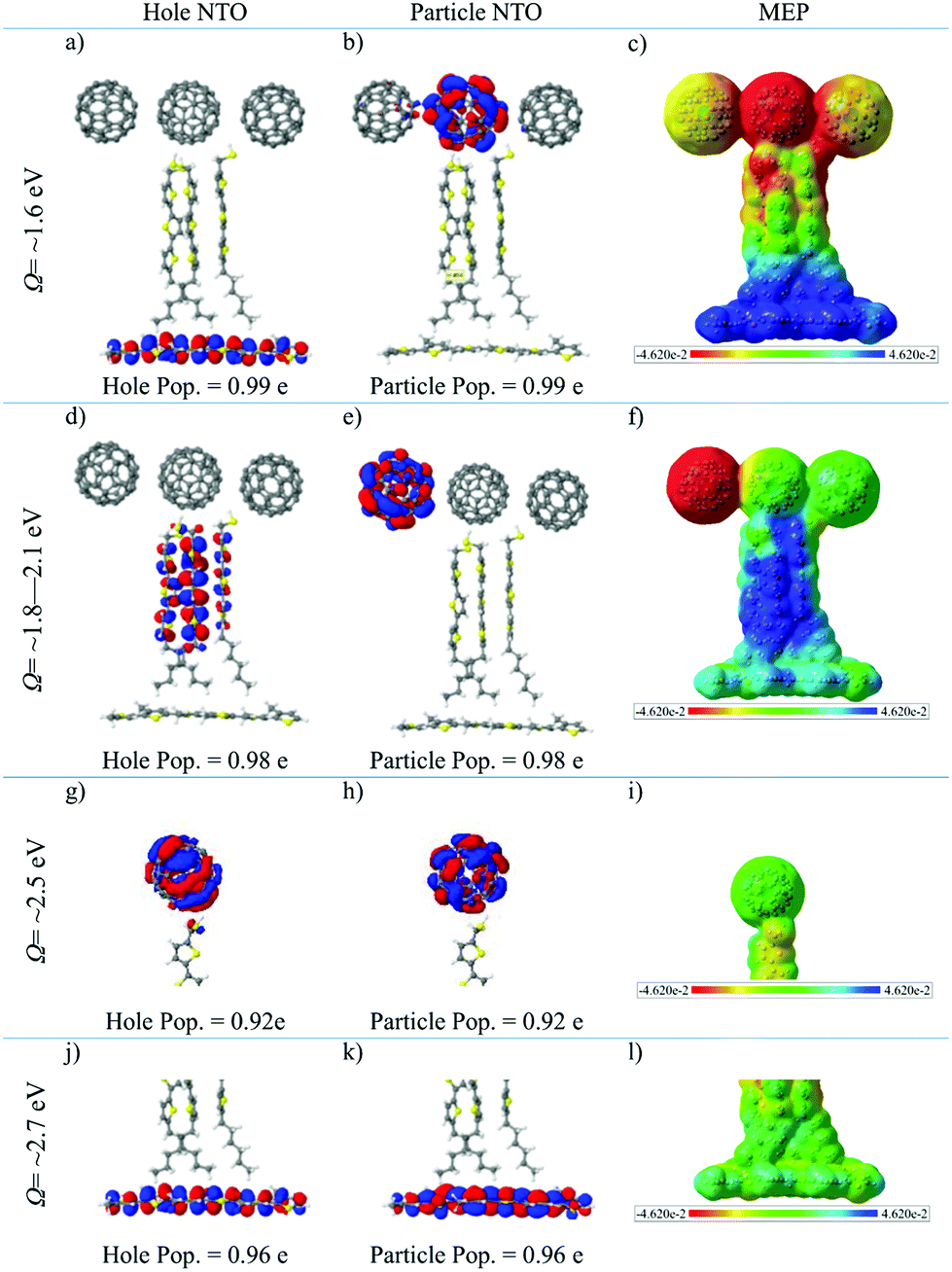

Fig. 4 Natural Transition Orbitals (NTO), particle/hole populations and molecular electrostatic potential (MEP) of (a, b, c) the lowest-energy P3HT → (C₆₀)₃ CT state, (d, e, f) the lowest-energy T3 → (C₆₀)₃ CT state, (j, k, l) the lowest-energy P3HT bright excitonic state of the extended thiophene trimer calculated using the CAM-B3LYP/6-31G method in the SS environment, and (g, h, i) the lowest-energy C₆₀ dark excitonic state of the isolated standard thiophene trimer calculated using the CAM-B3LYP/6-31G* method. Here we use NTO isovalue ±0.015 e per Bohr³ and MEP isovalue ±0.0003 e per Bohr³.

The next band consists of (T3)₃ → (C₆₀)₃ CT states. Here the lowest-energy state of this type (Fig. 4d and e) shows a transition from an occupied orbital diffusely distributed across the (T3)₃ unit to an orbital located on a single C₆₀ molecule in the (C₆₀)₃ unit. The MEP plot given in Fig. 4f depicts similar character to the P3HT → (C₆₀)₃ delocalized CT character, however as expected the positive region is spread over the T3 unit and P3HT is essentially neutral.

The C₆₀ exciton band is represented in Fig. 4g and h by the lowest-energy C₆₀ state calculated for the isolated standard trimer. This band is optically dark consisting of an excitation localized to the C₆₀ molecule, while the MEP plot (Fig. 4i) shows very little polarity, which is typical for neutral excitonic states. For the P3HT bright excitonic state, the primary contribution to the electronic excitation is localized on the P3HT unit (Fig. 4j and k). The MEP plot of this state displayed in Fig. 4l shows only little polarity.

4. Conclusions

Efficient operation of organic solar cells based on the BHJ architecture is ensured by tuning sophisticated organic–organic interfaces to align excitonic and charge transfer excited states to provide robust photo-generated exciton dissociation, while minimizing the recombination of the dissociated electron and hole across the donor–acceptor interface. The present study focuses on a detailed molecular model of a polar interface in a bulk heterojunction, which is suggested by our experiment. Here a self-assembled spacer unit (oligomer T3) is included in between a P3HT donor and C₆₀ acceptor materials. Following a non-trivial geometry optimization routine, extensive TD-DFT calculations based on long-range corrected functional mode and including environmental effects have been performed to characterize the series of lowest excited singlet states in terms of charge transfer and excitonic character. The calculations show unequivocally the strong stabilization of the CT states by environmental effects. The amount of stabilization increases with the distance of the charges (P3HT → C₆₀vs. T3 → C₆₀ CT) due to improved environmental stabilization. By comparison with a system of an ion pair without spacer layer (P3HT → C₆₀), a stabilization of more than 1 eV is computed for the single layer model. Inclusion of more layers are expected to increase the stabilization somewhat further but are currently too expensive in the framework of an explicit molecular model and state-specific TDDFT. Both spacer models show that with consideration of environmental interaction the lowest excited states are formed by bands of CT states, the lowest ones being of P3HT → C₆₀ character followed by T3 → C₆₀ transitions. The bright excitonic P3HT state is located 0.5 eV above the first CT below and 1.15 eV above the lowest CT state. Local C₆₀ excitations were found below the P3HT state, but significantly (∼0.9 eV) above the lowest CT state.

Such calculated and analyzed electronic structures fully support our hypothesis which emerged from experimental study:¹³ photo-generated exciton in the P3HT component at the BHJ interface either goes to C₆₀via energy transfer and subsequently dissociates into a T3 → C₆₀ CT state, or directly dissociates into a P3HT → C₆₀ state. This state is followed by a transition to the next P3HT → C₆₀ state with lower energy, which has even stronger CT character. Our calculation of the stability of the CT states clearly indicate via the use of eqn (1) that the spacer facilitates separation of the electron and hole, thus diminishing their Coulomb binding energy and reducing the efficiency of recombination. Moreover, our simulations demonstrate how the interface ordering and structure affects the energetics of relevant states via electronic coupling in self-assembled oligomer layers, which further translates to macroscopic device performance. Such physical processes are general and underpin manipulation in any donor–acceptor based electronic devices, such as organic light emitting diodes, photodetectors, sensors, and comprise the design principles for tailoring the interface properties of organic electronic devices. All our simulations of electronically excited states are based on the equilibrium molecular geometries. To capture the effects of vibrational broadening and conformational disorder, it is possible to use multiple snapshots of structures obtained from classical molecular dynamics simulations. However, modeling excited states in such a case is currently a numerically intractable task for the present high level of theory. Likewise, direct modeling of excited state relaxation with, for instance, surface hopping approaches,⁶² are numerically costly and require reduced Hamiltonian models. This work goes far beyond the scope of this paper and will be addressed in future investigations.

Conflicts of interest

The authors declare no competing financial interest.

Acknowledgements

The work at Los Alamos National Laboratory (LANL) was supported by the LANL LDRD program (W. N., H. T., A. D. M., S. T.). This work was done in part at Center for Nonlinear Studies (CNLS) and the Center for Integrated Nanotechnologies CINT, a U.S. Department of Energy and Office of Basic Energy Sciences user facility, at LANL. This research used resources provided by the LANL Institutional Computing Program. We also thank for computer time at the Linux cluster arran of the School for Pharmaceutical Science and Technology of the University of Tianjin, China.

References

1. B. C. Thompson and J. M. Frechet, Angew. Chem., Int. Ed., 2008, 47, 58–77.
2. Y. Liang, D. Feng, Y. Wu, S.-T. Tsai, G. Li, C. Ray and L. Yu, J. Am. Chem. Soc., 2009, 131, 7792–7799.
3. G. Yu, J. Gao, J. C. Hummelen, F. Wudl and A. J. Heeger, Science, 1995, 270, 1789–1791.
4. J.-L. Brédas, J. E. Norton, J. Cornil and V. Coropceanu, Acc. Chem. Res., 2009, 42, 1691–1699.
5. B. Baumeier, F. May, C. Lennartz and D. Andrienko, J. Mater. Chem., 2012, 22, 10971–10976.
6. Y. Kanai and J. C. Grossman, Nano Lett., 2007, 7, 1967–1972.
7. Y. Yi, V. Coropceanu and J.-L. Brédas, J. Am. Chem. Soc., 2009, 131, 15777–15783.
8. N. S. Sariciftci and A. J. Heeger, Int. J. Mod. Phys. B, 1994, 8, 237–274.
9. G. Grancini, M. Maiuri, D. Fazzi, A. Petrozza, H. J. Egelhaaf, D. Brida, G. Cerullo and G. Lanzani, Nat. Mater., 2013, 12, 29–33.
10. S. Gelinas, A. Rao, A. Kumar, S. L. Smith, A. W. Chin, J. Clark, T. S. van der Poll, G. C. Bazan and R. H. Friend, Science, 2014, 343, 512–516.
11. E. R. Bittner and C. Silva, Nat. Commun., 2014, 5, 3119.
12. E. Vella, H. Li, P. Gregoire, S. M. Tuladhar, M. S. Vezie, S. Few, C. M. Bazan, J. Nelson, C. Silva-Acuna and E. R. Bittner, Sci. Rep., 2016, 6, 29437.
13. W. Y. Nie, G. Gupta, B. K. Crone, F. L. Liu, D. L. Smith, P. P. Ruden, C. Y. Kuo, H. Tsai, H. L. Wang, H. Li, S. Tretiak and A. D. Mohite, Adv. Sci., 2015, 2, 1500024.
14. I. H. Campbell and B. K. Crone, Appl. Phys. Lett., 2012, 101, 023301.
15. S. Sampat, A. D. Mohite, B. Crone, S. Tretiak, A. V. Malko, A. J. Taylor and D. A. Yarotski, J. Phys. Chem. C, 2015, 119, 1286–1290.
16. C. Adamo and D. Jacquemin, Chem. Soc. Rev., 2013, 42, 845–856.
17. A. Dreuw, J. L. Weisman and M. Head-Gordon, J. Chem. Phys., 2003, 119, 2943–2946.
18. A. Dreuw and M. Head-Gordon, Chem. Rev., 2005, 105, 4009–4037.
19. B. Kaduk, T. Kowalczyk and T. Van Voorhis, Chem. Rev., 2012, 112, 321–370.
20. H. Iikura, T. Tsuneda, T. Yanai and K. Hirao, J. Chem. Phys., 2001, 115, 3540.
21. O. A. Vydrov and G. E. Scuseria, J. Chem. Phys., 2006, 125, 234109.
22. T. Stein, L. Kronik and R. Baer, J. Am. Chem. Soc., 2009, 131, 2818–2820.
23. A. W. Lange and J. M. Herbert, J. Am. Chem. Soc., 2009, 131, 3913–3922.
24. L. Kronik, T. Stein, S. Refaely-Abramson and R. Baer, J. Chem. Theory Comput., 2012, 8, 1515–1531.
25. T. Körzdörfer, J. S. Sears, C. Sutton and J.-L. Brédas, J. Chem. Phys., 2011, 135, 204107.
26. H. Li, R. Nieman, A. J. A. Aquino, H. Lischka and S. Tretiak, J. Chem. Theory Comput., 2014, 10, 3280–3289.
27. T. Yanai, D. P. Tew and N. C. Handy, Chem. Phys. Lett., 2004, 393, 51–57.
28. P. A. Limacher, K. V. Mikkelsen and H. P. Lüthi, J. Chem. Phys., 2009, 130, 194114.
29. J.-D. Chaia and M. Head-Gordon, Phys. Chem. Chem. Phys., 2008, 10, 6615–6620.
30. A. K. Manna, M. H. Lee, K. L. McMahon and B. D. Dunietz, J. Chem. Theory Comput., 2015, 11, 1110–1117.
31. I. Borges, A. J. a. Aquino, A. Köhn, R. Nieman, W. L. Hase, L. X. Chen and H. Lischka, J. Am. Chem. Soc., 2013, 135, 18252–18255.
32. K. Sen, R. Crespo-Otero, O. Weingart, W. Thiel and M. Barbatti, J. Chem. Theory Comput., 2013, 9, 533–542.
33. D. Balamurugan, A. J. A. Aquino, F. de Dios, L. Flores, H. Lischka and M. S. Cheung, J. Phys. Chem. B, 2013, 117, 12065–12075.
34. T. M. Perrine, T. Berto and B. D. Dunietz, J. Phys. Chem. B, 2008, 112, 16070–16075.
35. H. E. Katz, J. Mater. Chem., 1997, 7, 369–376.
36. J. Cornil, D. Beljonne, J. P. Calbert and J. L. Bredas, Adv. Mater., 2001, 13, 1053–1067.
37. J. L. Bredas, J. P. Calbert, D. A. da Silva and J. Cornil, Proc. Natl. Acad. Sci. U. S. A., 2002, 99, 5804–5809.
38. M. H. Lee, E. Geva and B. D. Dunietz, J. Phys. Chem. A, 2016, 120, 2970–2975.
39. M. H. Lee, B. D. Dunietz and E. Geva, J. Phys. Chem. Lett., 2014, 5, 3810–3816.
40. J. P. Perdew, K. Burke and M. Ernzerhof, Phys. Rev. Lett., 1996, 77, 3865–3868.
41. A. Schafer, H. Horn and R. Ahlrichs, J. Chem. Phys., 1992, 97, 2571–2577.
42. R. Ditchfield, W. J. Hehre and J. A. Pople, J. Chem. Phys., 1971, 54, 724–728.
43. G. A. Petersson, A. Bennett, T. G. Tensfeldt, M. A. Al-Laham, W. A. Shirley and J. Mantzaris, J. Chem. Phys., 1988, 89, 2193–2218.
44. G. A. Petersson and M. A. Al-Laham, J. Chem. Phys., 1991, 94, 6081–6090.
45. M. Cossi, N. Rega, G. Scalmani and V. Barone, J. Comput. Chem., 2003, 24, 669–681.
46. E. Runge and E. K. U. Gross, Phys. Rev. Lett., 1984, 52, 997–1000.
47. M. Petersilka, U. J. Gossmann and E. K. U. Gross, Phys. Rev. Lett., 1996, 76, 1212–1215.
48. R. Improta, V. Barone, G. Scalmani and M. J. Frisch, J. Chem. Phys., 2006, 125, 054103.
49. R. Ahlrichs, M. Bär, M. Häser, H. Horn and C. Kölmel, Chem. Phys. Lett., 1989, 162, 165–169.
50. M. J. Frisch, G. W. Trucks, H. B. Schlegel, G. E. Scuseria, M. A. Robb, J. R. Cheeseman, G. Scalmani, V. Barone, B. Mennucci, G. A. Petersson, H. Nakatsuji, M. Caricato, X. Li, H. P. Hratchian, A. F. Izmaylov, J. Bloino, G. Zheng, J. L. Sonnenberg, M. Hada, M. Ehara, K. Toyota, R. Fukuda, J. Hasegawa, M. Ishida, T. Nakajima, Y. Honda, O. Kitao, H. Nakai, T. Vreven, J. A. Montgomery Jr., J. E. Peralta, F. Ogliaro, M. J. Bearpark, J. Heyd, E. N. Brothers, K. N. Kudin, V. N. Staroverov, R. Kobayashi, J. Normand, K. Raghavachari, A. P. Rendell, J. C. Burant, S. S. Iyengar, J. Tomasi, M. Cossi, N. Rega, N. J. Millam, M. Klene, J. E. Knox, J. B. Cross, V. Bakken, C. Adamo, J. Jaramillo, R. Gomperts, R. E. Stratmann, O. Yazyev, A. J. Austin, R. Cammi, C. Pomelli, J. W. Ochterski, R. L. Martin, K. Morokuma, V. G. Zakrzewski, G. A. Voth, P. Salvador, J. J. Dannenberg, S. Dapprich, A. D. Daniels, Ö. Farkas, J. B. Foresman, J. V. Ortiz, J. Cioslowski and D. J. Fox, Gaussian 09, Gaussian, Inc., Wallingford, CT, USA, 2009.
51. A. V. Luzanov, A. A. Sukhorukov and V. É. Umanskii, Theor. Exp. Chem., 1976, 10, 354–361.
52. I. Mayer, Chem. Phys. Lett., 2007, 437, 284–286.
53. R. L. Martin, J. Chem. Phys., 2003, 118, 4775–4777.
54. F. Plasser and H. Lischka, J. Chem. Theory Comput., 2012, 8, 2777–2789.
55. F. Plasser, M. Wormit and A. Dreuw, J. Chem. Phys., 2014, 141, 024106.
56. F. Plasser, TheoDORE: a package for theoretical density, orbital relaxation, and exciton analysis, available from http://theodore-qc.sourceforge.net.
57. K. A. Smith, Y. H. Lin, J. W. Mok, K. G. Yager, J. Strzalka, W. Y. Nie, A. D. Mohite and R. Verduzco, Macromolecules, 2015, 48, 8346–8353.
58. C. Y. Kuo, Y. H. Liu, D. Yarotski, H. Li, P. Xu, H. J. Yen, S. Tretiak and H. L. Wang, Chem. Phys., 2016, 481, 191–197.
59. D. Credgington and J. R. Durrant, J. Phys. Chem. Lett., 2012, 3, 1465–1478.
60. G. Lakhwani, A. Rao and R. H. Friend, Annu. Rev. Phys. Chem., 2014, 65, 557–581.
61. C. A. Guido, D. Jacquemin, C. Adamo and B. Mennucci, J. Chem. Theory Comput., 2015, 11, 5782–5790.
62. J. C. Tully, J. Chem. Phys., 1990, 93, 1061–1071.

---

Footnote

† Electronic supplementary information (ESI) available: Tables of vertical excitations for the different models computed, Cartesian coordinates for the standard and extended trimer systems. See DOI: 10.1039/c7nr07125f

---