
 Open Access Article
 This Open Access Article is licensed under a
 Creative Commons Attribution 3.0 Unported Licence
Highly efficient surface hopping dynamics using a linear vibronic coupling model†
Felix
Plasser
 *ab,
Sandra
Gómez
b,
Maximilian F. S. J.
Menger
bc,
Sebastian
Mai
b and
Leticia
González
*b
*ab,
Sandra
Gómez
b,
Maximilian F. S. J.
Menger
bc,
Sebastian
Mai
b and
Leticia
González
*b
aDepartment of Chemistry, Loughborough University, Loughborough, LE11 3TU, UK. E-mail: F.Plasser@lboro.ac.uk
bInstitute for Theoretical Chemistry, Faculty of Chemistry, University of Vienna, Währingerstr. 17, 1090 Vienna, Austria. E-mail: leticia.gonzalez@univie.ac.at
cDipartimento di Chimica e Chimica Industriale, University of Pisa, Via G. Moruzzi 13, 56124 Pisa, Italy
First published on 3rd October 2018
Abstract
We report an implementation of the linear vibronic coupling (LVC) model within the surface hopping dynamics approach and present utilities for parameterizing this model in a blackbox fashion. This results in an extremely efficient method to obtain qualitative and even semi-quantitative information about the photodynamical behavior of a molecule, and provides a new route toward benchmarking the results of surface hopping computations. The merits and applicability of the method are demonstrated in a number of applications. First, the method is applied to the SO2 molecule showing that it is possible to compute its absorption spectrum beyond the Condon approximation, and that all the main features and timescales of previous on-the-fly dynamics simulations of intersystem crossing are reproduced while reducing the computational effort by three orders of magnitude. The dynamics results are benchmarked against exact wavepacket propagations on the same LVC potentials and against a variation of the electronic structure level. Four additional test cases are presented to exemplify the broader applicability of the model. The photodynamics of the isomeric adenine and 2-aminopurine molecules are studied and it is shown that the LVC model correctly predicts ultrafast decay in the former and an extended excited-state lifetime in the latter. Futhermore, the method correctly predicts ultrafast intersystem crossing in the modified nucleobase 2-thiocytosine and its absence in 5-azacytosine while it fails to describe the ultrafast internal conversion to the ground state in the latter.
1 Introduction
The trajectory surface hopping method1 is a powerful computational tool that allows for the study of quantum transitions occurring during ultrafast molecular photodynamical processes. Using this method, a variety of processes occurring within one spin multiplicity have been studied, such as the primary event in vision,2 photodeactivation of nucleobases3 and other biological chromophores,4 as well as photochemical organic reactions5 and photocatalysis.6 Even more, through an extension of this formalism to include spin–orbit coupling (SOC),7 it has been possible to elucidate intersystem crossing (ISC) processes in a variety of molecules, e.g. modified nucleobases,8 nitroaromatics,9,10 and transition metal complexes.11 Notwithstanding their popularity,12–18 standard ab initio surface hopping approaches suffer from two downsides, their high computational cost and the difficulty of verifying whether the approximations made when going from the quantum to the quasiclassical description are appropriate. The high computational cost stems from the ab initio computations carried out at every time step of every trajectory, often requiring hundreds of thousands of such calculations for the whole ensemble. Because of this high cost, the simulation of large molecules, long-time dynamics, and rare events is often not feasible. Furthermore, the need of a large amount of on-the-fly computations often requires that cheaper but less accurate electronic structure methods are employed, possibly deteriorating the quality of the results.Different strategies have been developed for reducing the number of electronic structure computations in trajectory dynamics simulations. These include a parameterization of the surfaces through interpolated diabatic Hamiltonians,19,20 on-the-fly constructed databases,21,22 or artificial neural networks.23,24 However, none of these approaches is in routine use, which probably derives from the fact that they do require a significant amount of electronic structure computations and expert knowledge to be applied successfully. Here, we want to proceed in a different way and combine the surface hopping method with a very popular approach that is in routine use and has been well-tested and refined by numerous groups over the last 30 years, the vibronic coupling (VC) model.25 VC models provide a description of the main physics of interacting potential surfaces, including the conical shape of their intersections, using only a minimum number of parameters with clear physical meaning. They can be parameterized using standardized protocols25–29 and are commonly used in the context of quantum dynamics, in particular within the well-established multiconfigurational time-dependent Hartree (MCTDH) method,30 and have been shown to be powerful for describing ultrafast nonadiabatic processes in organic and inorganic molecules,31–34 in transition metal complexes27,35,36 and at interfaces.37 Despite the huge popularity of surface hopping and VC models individually, it is difficult to find any combined application of both methods in the literature,38 and certainly no generally applicable implementation is available. However, such a combination will be highly desirable as it allows speeding up surface hopping simulations by orders of magnitude when compared to on-the-fly dynamics and allows for including essentially an unlimited number of degrees of freedom as opposed to quantum dynamics. At the same time, it does not introduce any new approximation that is not already included in either one of the two well-tested constituent methods. If a particular photophysical problem can be described by both methods individually it should also be described correctly by the combined approach. Conversely, as we will discuss below, the method provides a convenient and versatile approach for evaluating the reliability of its different ingredients such as the electronic structure data, the surface hopping algorithm, and the parameterized potential energy surfaces. Finally, it offers a new route for evaluating the influence of different degrees of freedom in VC models used in quantum dynamics. For the above reasons, we deem a general implementation of LVC surface hopping highly desirable.
With this motivation in mind, we created a general interface for performing surface hopping dynamics using VC models within the SHARC (surface hopping with arbitrary couplings) molecular dynamics package.7,17,39,40 In this work, we investigate the simplest possible case, i.e., a VC model using only linear terms (LVC) parameterized using only a single excited-state computation, and study its usefulness for addressing various photophysical problems. First, sulfur dioxide (SO2) is studied, a molecule that has recently attracted significant attention,34,41–46 due to its ultrafast ISC occurring on a subpicosecond time scale. Here, we investigate whether the employed LVC model can predict the occurrence of ultrafast ISC and whether it correctly describes the participation of the different electronic states, a question that has been open since decades47 and was clarified only a few years ago.41,44 Second, adenine and its structural isomer 2-aminopurine (2AP) are investigated. The remarkable feature of these two molecules is that despite their structural similarity, they exhibit a completely different photophysical behavior.48,49 Adenine undergoes non-radiative decay on a subpicosecond time scale,50–54 whereas the closely related 2AP system possesses an extended excited state lifetime (>100 ps) in gas phase55 and is even fluorescent in many solvents.48,56 We examine whether the presented SHARC/LVC approach allows discriminating between these qualitatively different behaviours. As a third test case, the modified nucleobase 2-thiocytosine (2TC) is investigated. 2TC belongs to the class of thio-nucleobases, which have been the target of much research57–60 due to their interesting photophysical properties based on their remarkably ultrafast ISC. In 2TC, ISC occurs on a 200–400 fs time scale,58 whereas virtually no decay to the S0 occurs. Finally, we investigate 5-azacytosine (5AC), which is the chromophore of the widespread anti-cancer drug azacytidine.61 As its mechanism of action involves incorporation into DNA, its photophysics is of interest regarding drug-induced light sensitivity and the crucial feature is that it undergoes decay to the ground state rather than ISC.62,63
2 Methods
2.1 Wavefunction representations
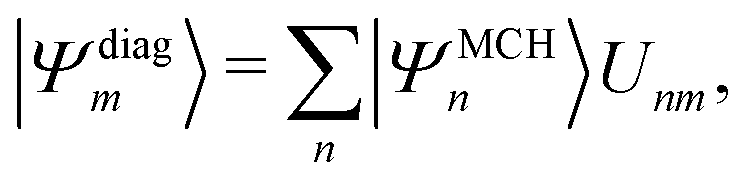
For the following discussion, it is beneficial to briefly review the different possible representations of electronic wavefunctions and establish the naming conventions39,64 used in the rest of the paper, see Fig. 1. Standard quantum chemistry codes deal with an electronic Hamiltonian that includes molecular Coulomb interactions but neither external fields nor SOC. We label this operator the molecular Coulomb Hamiltonian (MCH) and its eigenfunctions form the MCH representation (Fig. 1(b)). In the MCH representation, the states possess a distinct multiplicity and are labelled S1, S2, …,T1, T2, … States of the same spin-multiplicity do not cross in a one-dimensional picture whereas states of different multiplicities do. The Hamiltonian including SOC is termed the “total Hamiltonian” and its eigenfunctions, generally possessing mixed spin, form the “diagonal” representation (Fig. 1(c)). These states do not cross in a one-dimensional picture and can be labelled with numbers 1, 2, …, etc. An alternative way of transforming the MCH states is by minimizing nonadiabatic interactions leading to states of almost constant character in the diabatic representation (Fig. 1(a)). To indicate the diabatic representation, we either use symmetry labels (1B1, 1A2) or labels describing the state character (1ππ*, 1nπ*). | ||
| Fig. 1 Wavefunction representations used in this work: (a) the diabatic representation, which is the basis for the LVC model and used in the MCTDH dynamics, (b) the MCH representation, which is used in standard quantum chemical codes and is the input for SHARC, and (c) the diagonal representation, which is used during the SHARC dynamics. | ||
Per construction, the LVC model works in the diabatic basis. It is worth noting that MCTDH works entirely in the diabatic basis and can directly take the LVC model as input. In contrast, SHARC expects input in the MCH representation and propagates the wavefunction in the diagonal picture. It will be, thus, necessary to transform the input as described below (Section 2.5). The SHARC output can be given in any of the three pictures explained above, and it is, thus, possible to perform a one-to-one comparison with MCTDH despite the fact that different representations were used for the wavefunction propagation.
2.2 The linear vibronic coupling model
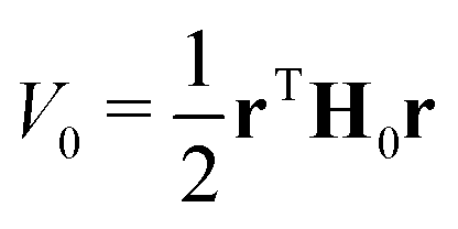
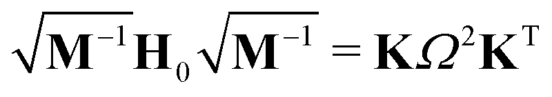
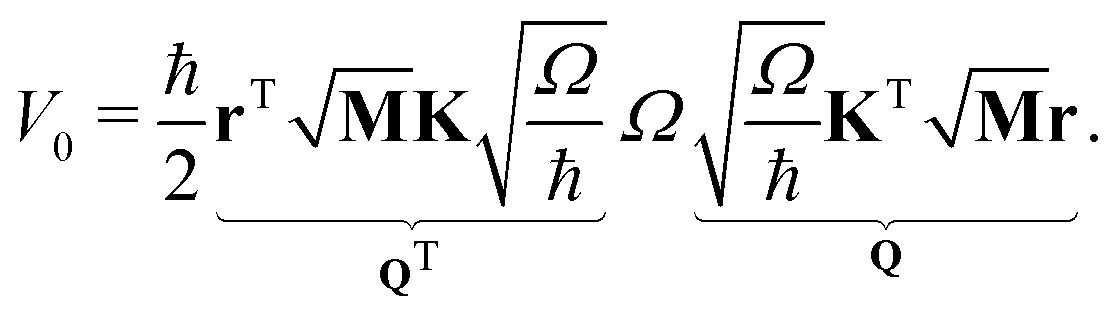
In a VC model the molecular Coulomb Hamiltonian operator, as defined above, is constructed in a diabatic representation as| V = V01 + W | (1) |
 | (2) |
 | (3) |
| Ω2 = diag(ω12, ω22, …,ω3N2), | (4) |
 | (5) |
 | (6) |
 | (7) |
Within the current work, an LVC model is considered, which contains the following state-specific terms in the W matrix.
 | (8) |
 | (9) |
2.3 Parameterization
In this work, we investigate the applicability of a “one-shot” LVC approach, i.e., using a parameterization that derives only from a single excited-state electronic structure computation. For this purpose, a new module was added to the SHARC molecular dynamics package17,40 that allows determining all parameters of the LVC model using only a ground-state frequency computation and a single-point calculation of excited-state energies, gradients, nonadiabatic couplings, and SOCs at the equilibrium geometry. The advantages of this module are that it works in a blackbox fashion, even in the case of many degrees of freedom, a high density of excited states, and the absence of symmetry.65In the “one-shot” LVC approach, the ωi values are simply the ground state vibrational frequencies while the εn energies and diabatic SOC constants are the vertical excitation energies and SOCs at the equilibrium geometry, respectively. The intrastate vibronic coupling constants are computed as the derivative of the electronic energy En of state n with respect to a normal mode25,27 computed at the reference geometry, which using eqn (6) can be rearranged as
 | (10) |
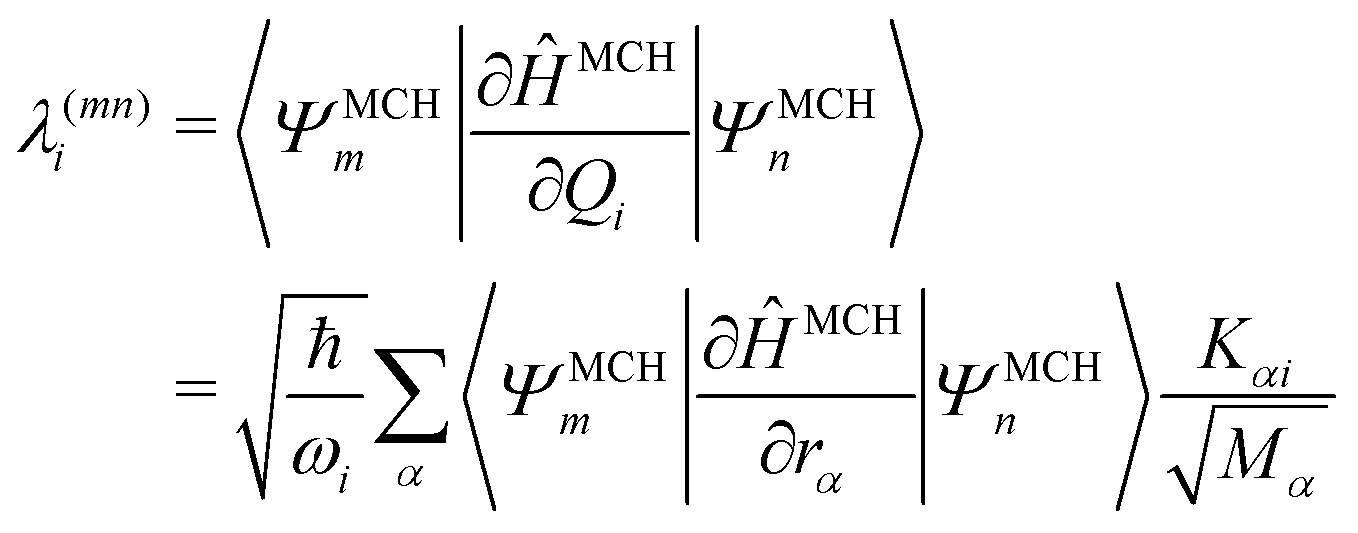 | (11) |
Commonly, the λ parameters are evaluated indirectly using energy-based information only, by considering either the excited state Hessian25,27,34 or by fitting the potential energy surfaces to model potentials.28,29 However, following arguments by Yarkony and coworkers,66 it is possible to evaluate eqn (11) directly and this approach is used here. In the case of configuration interaction (CI) computations, the 〈ΨMCHm|∂ĤMCH/∂rα|ΨMCHn〉 terms can be obtained from derivatives of the CI-matrix yielding a quantity termed fCI that is closely related to the nonadiabatic coupling vector.66,67 Similar equations have also been incorporated within coupled cluster theory.68,69 In cases where nonadiabatic coupling vectors are not available, it is possible to compute the λ(mn)i values in the same spirit through a numerical differentiation using a recently described algorithm65 based on wavefunction overlaps.70
An LVC model, even when constructed in this simple way, provides qualitatively correct potential energy surfaces in the vicinity of the expansion point and assures the proper conical topology of intersections between adiabatic states. However, the quality of the description is expected to deteriorate if the molecule undergoes large-amplitude structural changes, such that anharmonicities and higher-order vibronic coupling terms become important. As a consequence, it is not expected that the presented protocol is adequate in describing all photochemical reactions or other processes involving strong structural rearrangements. In these cases, it may be possible to resort to higher-order VC models and more sophisticated parameterization schemes26,28 or on-the-fly dynamics will have to be applied. On the other hand, we expect that the simple “one-shot” LVC approach can provide a qualitatively correct description of photophysical processes, like internal conversion and ISC, that are dominated by the electron dynamics and do not involve the breaking or creation of chemical bonds or the motion of flexible groups. In Section 3, we investigate the applicability of this method for the description of a number of realistic photophysical processes and find remarkably good agreement with experiment as well as with more expensive computational protocols.
2.4 SHARC dynamics
The SHARC method, used for propagating dynamics on coupled surfaces of different multiplicity has been recently reviewed in ref. 17. For completeness, we provide here a brief overview. The nuclei follow classical trajectories obtained by integrating Newton's equation: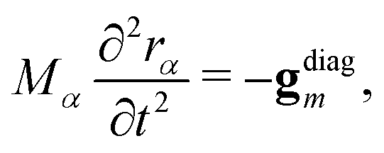 | (12) |
 | (13) |
 | (14) |
| Hdiag = U†HMCHU, | (15) |
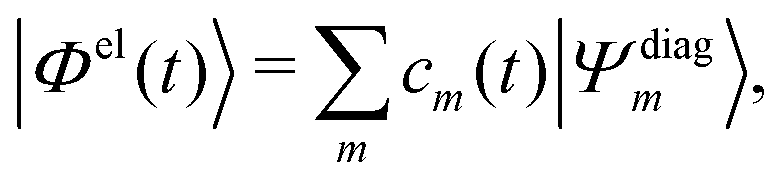
Practically, with the above diagonalization carried out, the coefficients cm(t) can be propagated according to the matrix equation
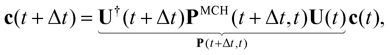 | (16) |
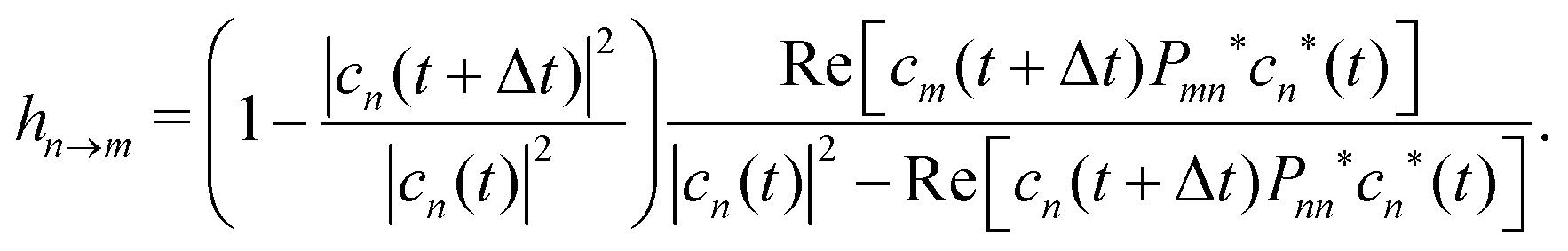 | (17) |
In this work, the gradient gdiagm of the diagonal state, needed to propagate eqn (12), is approximated as a linear combination of the MCH gradients
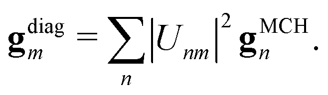 | (18) |
As in other surface hopping approaches, after a successful hop the nuclear momenta are adjusted to conserve total energy and by default the full velocity vector is rescaled. Furthermore, the electronic coefficients are adjusted after each time step to consider decoherence; here we use the well-established energy-based decoherence correction introduced by Granucci et al.72
2.5 Interface to SHARC
All quantities required by the SHARC dynamics program can be constructed from the LVC model using the workflow sketched in Fig. 2. First, the normal mode displacements are computed from the Cartesian geometry according to eqn (6). Then, the potential matrix V is computed using eqn (7)–(9) and subsequently diagonalized according toVT = T![[thin space (1/6-em)]](https://www.rsc.org/images/entities/char_2009.gif) diag(E1, …, ENst) diag(E1, …, ENst) | (19) |
| S(t,t + Δt) = T(t)TT(t + Δt). | (20) |
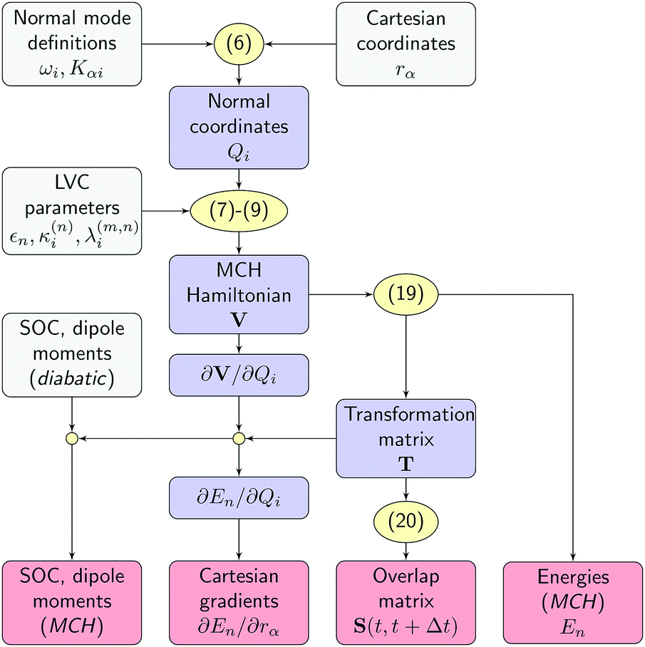 | ||
| Fig. 2 Workflow of the SHARC/LVC method. Input quantities, intermediates and output are given in grey, blue, and red boxes, respectively. Equation numbers are shown in yellow. | ||
In summary, the new interface provides all quantities in the MCH basis and in Cartesian coordinates, so that for the SHARC dynamics driver the simulations do not differ from on-the-fly simulations. This also means that all analysis procedures implemented in SHARC, considering, for example, Cartesian coordinates and electronic populations, can automatically be applied to the LVC-based simulations.
Technically speaking, in our original implementation the time-determining step was not the evaluation of the matrix operations but the communication between the Fortran SHARC driver and the LVC program written in Python. Therefore, a new driver for SHARC – called PySHARC – was developed within the course of this project, utilizing Python's C API (application program interface), thus allowing for in-memory communication between the Python interface and SHARC's Fortran routines, replacing the file based communication used so far. Additionally, the new implementation makes it possible to read all parameters just once and store them in memory reducing the number of file operations to be performed and enhancing efficiency even further.
2.6 Computational details
Electronic structure computations on SO2 were carried out at two different levels of theory: (i) multireference configuration interaction (MR-CI)74 including single excitations using a complete active space of 6 active electrons in 6 orbitals as reference space, and a polarized double-ζ basis set of ANO-RCC75 type [MR-CIS(6,6)/VDZP] following ref. 43, and (ii) MR-CI with single and double excitations using a larger (12,9) active space and a polarized triple-ζ basis set75 [MR-CISD(12,9)/VTZP]. In both cases, the orbitals were generated at the complete-active space self-consistent field level considering 12 electrons in 9 orbitals, CASSCF(12,9). Scalar relativistic effects were taken into account by using the second-order Douglas–Kroll–Hess Hamiltonian76 while SOC was included through atomic mean-field integrals77,78 and MR-CI SOC values were computed in a perturbative fashion.79 The κ parameters were computed from analytical MR-CI gradients80 and the λ parameters were computed through derivatives of CI matrix elements.67 In the case of adenine and 2AP, the MR-CIS computations were performed using an active space of 10 electrons in 8 orbitals (2 × n, 3 × π, 3 × π*) and the aug-cc-pVDZ81 basis set. In the case of 2TC an active space of 10 electrons in 8 orbitals (1 × n, 4 × π, 3 × π*) was used for generating the orbitals with CASSCF while a (6,5) reference space was used for MR-CIS. For 5AC orbitals were generated using CASSCF(12,9) (2 × n, 4 × π, 3 × π*) and again a (6,5) reference space was used for MR-CIS. In both cases the cc-pVDZ basis set81 was used. MR-CI computations were performed with the COLUMBUS program system82–84 using integrals generated with MOLCAS85 for SO2, 2TC, and 5AC and with DALTON86 for adenine and 2AP.The optical absorption spectrum of SO2 was computed according to a Wigner distribution of the ground state zero-point vibrational wavefunction,87 using normal modes computed at MR-CIS level. The surface hopping dynamics simulations on SO2 were started according to the excitation windows indicated as grey rectangles in Fig. 3 (4.1–4.6 eV for MR-CIS and 3.9–4.4 eV for MR-CISD). 4 singlet and 3 triplets states were considered in the dynamics and 200 trajectories, each, were propagated on the MR-CIS and MR-CISD potentials. A time step length of 0.5 fs and a locally diabatic method for wavefunction propagation were used.71 An energy-based decoherence correction (C = 0.1 H) was used.72 For MCTDH,30 the vibrational ground state wavefunction was promoted to the diabatic 1B1 state and the dynamics was propagated for 700 fs using 10 single particle functions per normal mode, each expressed through 32 Legendre polynomials. UV absorption spectra were computed as the Fourier transform of the autocorrelation function obtained from the MCTDH dynamics and shifted by the zero-point energy of 0.1915 eV.
In the case of adenine the excitation window was chosen as 6.1 ± 0.1 eV and 209 trajectories were propagated for 1000 fs considering 5 singlet states. For 2AP the excitation window was chosen as 5.0 ± 0.1 eV and 163 trajectories were propagated for 50 ps considering 5 singlet states. The other set-up parameters (e.g., time step, propagator, decoherence correction) were kept as in the previous case. The normal modes used to construct the LVC model and to create the Wigner distribution were obtained at the RI-MP2/aug-cc-pVDZ level of theory using TURBOMOLE.88 For adenine and 2AP, relaxation time constants for the S2 → S1 and S1 → S0 processes were obtained by fitting a sequential first-order kinetics model to the population data. Errors of the time constants were obtained with the bootstrapping method,89 using 1000 bootstrapping samples for each ensemble (see S5 in the ESI† for more details on the fitting procedure). Note that these errors only describe the uncertainty due to the finite size of the trajectory ensembles but they make no statement about errors due to the electronic structure and dynamics methods.
The excitation windows chosen for 2TC and 5AC were 4.0 ± 0.1 eV and 5.0 ± 0.2 eV, respectively, and in both cases 200 trajectories were computed. The normal modes were computed at the respective MR-CIS levels.
3 Results and discussion
3.1 Sulfur dioxide
The new method is exemplified first for SO2, for which the absorption spectrum as well as ultrafast ISC dynamics are investigated. The triatomic SO2 molecule is a convenient test case, as high level on-the-fly dynamics43 as well as full-dimensional quantum dynamics44 have been performed and can be used as a reference. Table 1 presents the vertical excitation energies computed for the equilibrium geometry for the MR-CIS(6,6)/VDZP and MR-CISD(12,9)/VTZP levels of theory (see Computational details). The MR-CIS level shows that the S1 state (1B1) located at 4.46 eV is the only state below 6 eV possessing oscillator strength. The S2 state (1A2) is slightly higher in energy at 4.85 eV and symmetry-forbidden. The S3 state (1B2) is well-separated and lies close to 7 eV. The T1 state (3B1) is significantly lower in energy than any singlet state while T2 (3B2) and T3 (3A2) are energetically close to the S1 and S2 states. The ordering of the states at the MR-CISD level agrees well with that of MR-CIS but the MR-CISD values are consistently down-shifted by 0.2–0.3 eV.| State | MR-CIS | MR-CISD | |
|---|---|---|---|
| S1 | 1B1 | 4.463 (0.0029) | 4.227 (0.0055) |
| S2 | 1A2 | 4.848 | 4.595 |
| S3 | 1B2 | 6.805 (0.0931) | — |
| T1 | 3B1 | 3.650 | 3.350 |
| T2 | 3B2 | 4.478 | 4.211 |
| T3 | 3A2 | 4.627 | 4.356 |
Next, optical absorption spectra were computed for SO2. The original spectrum, computed from 1000 individual MR-CIS computations and initially reported in ref. 43, is shown in Fig. 3(a). This spectrum is somewhat blue-shifted with respect to the experiment90 (green line) but the spectral width is approximately reproduced. Next, the spectrum was recomputed using the LVC model constructed at the MR-CIS level [Fig. 3(b)]. As explained above, all parameters for this model (see Tables S1–S4, ESI†) were extracted from one single-point calculation at the equilibrium geometry. Remarkably, the LVC spectrum reproduces the full ab initio result very well in terms of location of the peak, its width, and the amount of contribution of the S2 state, with a fraction of the computational effort. For comparison, the absorption spectrum was also computed using the MCTDH method. This spectrum, shown in Fig. 3(c), exhibits a fine structure that cannot be obtained with semiclassical methods, but otherwise it agrees on the position and overall broadening. Employing the LVC model allows us to compute the spectrum also at the computationally much more expensive MR-CISD level, as presented in Fig. 3(e). This spectrum is red-shifted with respect to MR-CIS by about 0.2 eV, in agreement with Table 1, but otherwise the spectral shape is very similar. The MCTDH spectrum computed at the LVC(MR-CISD) level is presented in Fig. 3(f) showing a somewhat altered fine structure when compared to the MCTDH/LVC(MR-CIS) spectrum.
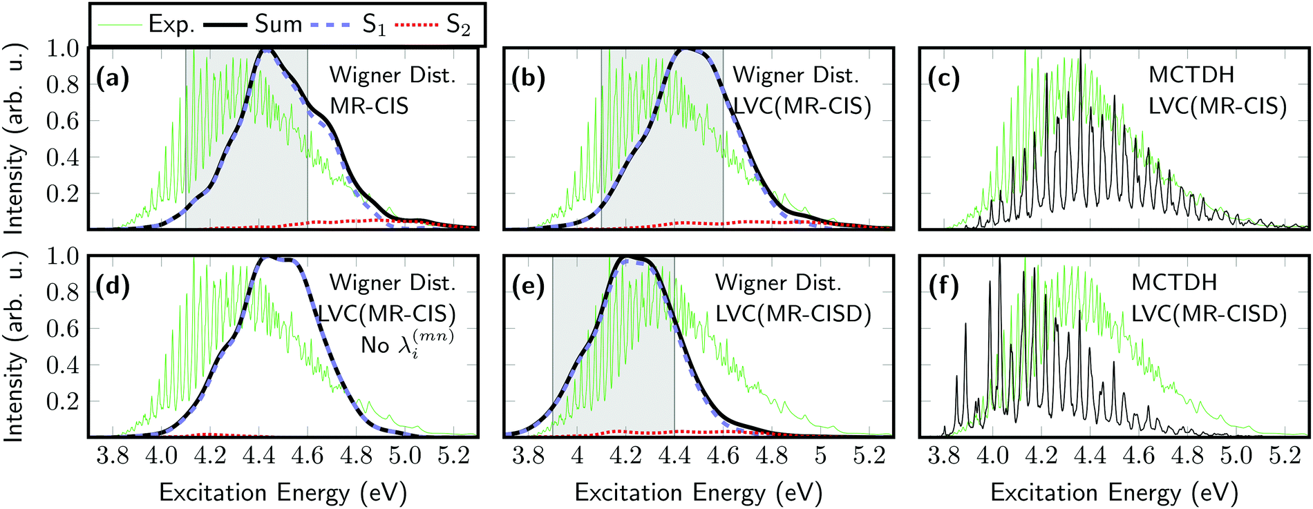 | ||
| Fig. 3 Absorption spectrum of SO2 computed using six different computational protocols: sampling of the Wigner distribution using (a) 1000 individual MR-CIS(6,6)/VDZP computations and LVC models constructed at the (b) MR-CIS(6,6)/VDZP and (e) MR-CISD(12,9)/VTZP levels; spectra computed from MCTDH dynamics using the (c) LVC(MR-CIS) and (f) LVC(MR-CISD) models. For comparison, the LVC(MR-CIS) spectrum without interstate coupling parameters is shown in (d). The excitation windows used for initial condition generation in the surface hopping simulations are marked as grey boxes in (a), (b), and (e). | ||
An important observation regarding the spectra presented above is that the adiabatic S2 state gains some intensity and contributes to the spectrum at higher energies. This feature clearly violates the Condon approximation as the S2 state is dark at the equilibrium geometry and, therefore, illustrates that the present protocol is able to compute spectra going beyond the Condon approximation. Hence, it is interesting to compare the spectra shown above with an LVC model that ignores the interstate couplings λ(mn)i. This corresponds to an approximation termed “vertical gradient”,91 meaning that the ground and excited state frequencies are the same, the oscillator strengths are constant, and only gradient information is used to construct the spectrum. This spectrum is shown in Fig. 3(d) and resembles that obtained using the full LVC model [Fig. 3(b)] with the exception that the high-energy shoulder deriving from the adiabatic S2 state cannot be reproduced.
As a next step, nonadiabatic dynamics simulations considering 4 singlet and 3 triplet states were performed for five of the computational protocols introduced in Fig. 3. These correspond to SHARC dynamics at the on-the-fly MR-CIS, LVC(MR-CIS), and LVC(MR-CISD) levels, as well as MCTDH simulations at the LVC(MR-CIS) and LVC(MR-CISD) levels. Here, the difference in computational effort is noteworthy: while the 111 on-the-fly MR-CIS trajectories from ref. 43 propagated for 700 fs required about 15000 core hours on a modern CPU, the parameterization and all 200 trajectories at the LVC(MR-CIS) level were finished in about 6 core hours using the PySHARC implementation. To be able to compare results between SHARC and MCTDH we use the diabatic (spectroscopic) representation,39i.e., we expand the time-dependent electronic wavefunctions in terms of the electronic states of the symmetric equilibrium geometry using a procedure described in more detail in ref. 43. The results of the on-the-fly SHARC simulations at the MR-CIS level, originally reported in ref. 43, are shown in Fig. 4(a). The initial excitation goes predominantly to the 1B1 state, which is the S1 state at the Franck–Condon geometry and the only symmetry-allowed state in the employed excitation window. Subsequently, the excited molecule stays on the S1 surface but an ultrafast change in diabatic character to 1A2 occurs making 1A2 the dominant state character already after 10 fs. Population of the triplet states is also ultrafast and after 700 fs the total triplet population amounts to 55%. The LVC model [Fig. 4(b)] reproduces the main features of the on-the-fly simulations. The initial inversion between the 1B1 and 1A2 characters occurs at exactly 10 fs. Sub-picosecond triplet population is observed as well, where most population is received by the 3B2 state, in agreement with ref. 43 and 44. However, ISC is somewhat slower than in the on-the-fly calculations, and after 700 fs only 38% triplet population is reached. The reduced population of the triplet states can be explained by the fact that ISC is most efficient during strong elongation of the S![[double bond, length as m-dash]](https://www.rsc.org/images/entities/char_e001.gif) O bonds,43 which is difficult to describe using LVC potentials. Nonetheless, it is remarkable that the dynamics of SO2 including all the involved states and timescales can be qualitatively described by the LVC model, especially considering that the nature of the involved states was still under dispute until few years ago.41,44
O bonds,43 which is difficult to describe using LVC potentials. Nonetheless, it is remarkable that the dynamics of SO2 including all the involved states and timescales can be qualitatively described by the LVC model, especially considering that the nature of the involved states was still under dispute until few years ago.41,44
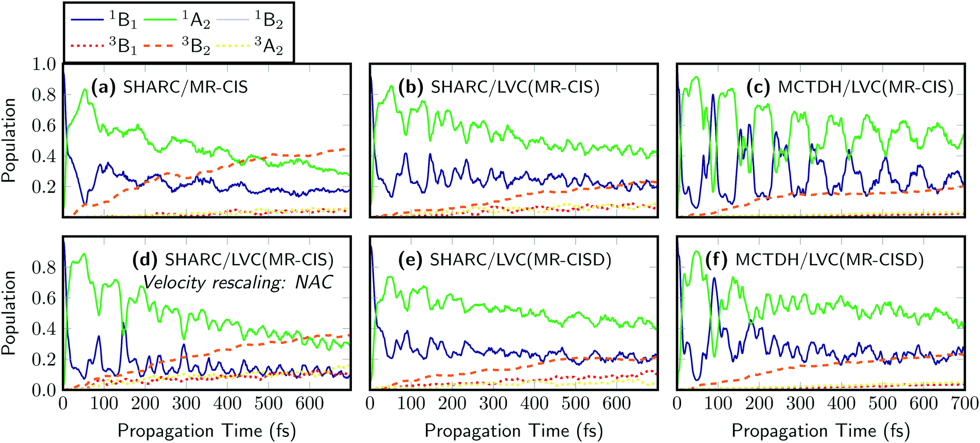 | ||
| Fig. 4 Time evolution of the diabatic singlet and triplet state populations of SO2 computed using six different computational protocols: (a) on-the-fly surface hopping, LVC surface hopping considering velocity rescaling parallel to (b) the velocity and (d) the nonadiabatic coupling, and (c) MCDTH, all based on MR-CIS(6,6)/VDZP potentials; (e) LVC surface hopping and (f) MCTDH, both based on MR-CISD(12,9)/VTZP potentials. | ||
The LVC method also directly allows judging the impact of quantum effects that cannot be captured by the surface hopping method. For this purpose quantum dynamics using the MCTDH method have been carried out for the LVC(MR-CIS) model, see Fig. 4(c). The results are very similar to the corresponding SHARC simulations [Fig. 4(b)] with the exception that stronger and more persistent oscillations between the singlet states are observed for MCTDH and that the triplet yield is somewhat lowered (only 27% after 700 fs).
A further advantage of the SHARC/LVC method is that it is possible to directly investigate the effects of different parameters and algorithmic choices in the surface hopping method to see whether they affect the agreement between SHARC and MCTDH. To exemplify this, we changed one algorithmic detail in the SHARC dynamics. In many SHARC applications, to conserve energy after a surface hop, typically the full velocity vector is rescaled. If nonadiabatic coupling vectors are available, a more rigorous alternative1,16 is to rescale only the component of the velocity parallel to the nonadiabatic coupling vector that induced the hop. The results of dynamics using this procedure are presented in Fig. 4(d). The different mode of rescaling leaves the qualitative picture unchanged but does affect the quantitative outcomes quite strongly. In particular, the triplet population after 700 fs is raised to 61%, which is twice as high as the MCTDH reference for the LVC(MR-CIS) potentials shown in Fig. 4(c). In addition, the oscillations between the singlet states are somewhat enhanced. It is noteworthy that the surface hopping results are so strongly affected by a seemingly innocuous algorithmic choice such as the mode of velocity rescaling. In the future, it will be thus of significant interest to evaluate the influence of other similar choices such as the treatment of frustrated hops and different options for decoherence corrections. The SHARC/LVC protocol provides an ideal way to perform such an evaluation for realistic high-dimensional systems, and a more detailed comparison of SHARC and MCTDH results is currently in progress in our group.
The efficiency of the LVC method allows for a significant improvement of the computational level in terms of the excitation level, active space, and one-electron basis set to perform dynamics at the MR-CISD(12,9)/VTZP level [Fig. 4(e)], which is not feasible for on-the-fly dynamics. One can see that at this level of theory, the 1B1/1A2 inversion happens somewhat slower and the populations are equal only after 15 fs owing to the fact that the magnitude of the λ value coupling these two states is reduced from 0.20 eV to 0.15 eV (cf. Tables S1 and S2, ESI†). Otherwise the dynamics is very similar, giving 38% triplet population after 700 fs. The MCTDH results computed using the LVC(MR-CISD) potentials are presented in Fig. 4(f). In this case, the 1B1/1A2 inversion occurs after 11.5 fs and the triplet yield after 700 fs amounts to 31%.
The MCTDH results shown here also compare well with the results of Lévêque et al. who used a more extended model Hamiltonian.44 In ref. 44 a similar oscillatory behaviour and a triplet yield of about 30% after 700 fs is reported. The main difference is that more persistent oscillations are observed in the present MCTDH/LVC(MR-CIS) dynamics. In a more general sense, the similarity of panels (b), (c), (e), and (f) suggests that neither the electronic structure level nor quantum effects play a decisive role in terms of the timescales or the states involved. On the other hand, a comparison with panel (a) shows that the inclusion of realistic on-the-fly potentials does have a notable effect on the triplet yield.
3.2 Adenine and 2-aminopurine
To evaluate the general applicability of the SHARC/LVC method to larger molecular systems, the adenine and 2AP molecules are investigated. In this case, it is of particular interest to investigate whether it is possible to correctly predict the qualitative differences in the photophysics of these two molecules, i.e., that adenine undergoes subpicosecond non-radiative decay50–54 whereas the closely related 2AP system possesses a more extended excited state lifetime (>100 ps).48,55,56 The MR-CIS vertical excitation energies for adenine and 2AP are presented in Table 2. The results obtained for adenine are similar to previous studies employing the MR-CIS method.52,92 The first singlet state, slightly below 6 eV is of nπ* character. Two ππ* states follow above 6 eV, the bright 1La state and the weakly absorbing 1Lb state, and S4 is again of nπ* character. These energies are consistently about 1 eV above the experimental and computational gas phase reference values,49,93 but as the shift is systematic and in view of the successful applicability of previous MR-CIS simulations to describe the photodynamics of adenine,52,92 we rely confidently on the suitability of the method. In Table 2 also the vertical excitation energies of 2AP are shown. The first excited states lie at lower energies than in the case of adenine and two states below 5 eV are present, possessing nπ* and ππ* character. The lower onset of absorption in 2AP is consistent with previous studies with the exception that the ππ* state is usually considered to be the lowest state.49,94,95| State | Ade | State | 2AP | |
|---|---|---|---|---|
| S1 | 11nπ* | 5.677 (0.000) | 11nπ* | 4.782 (0.003) |
| S2 | 11ππ* | 6.142 (0.329) | 11ππ* | 4.991 (0.112) |
| S3 | 21ππ* | 6.422 (0.055) | 21nπ* | 5.956 (0.001) |
| S4 | 21nπ* | 6.764 (0.006) | 21ππ* | 6.590 (0.231) |
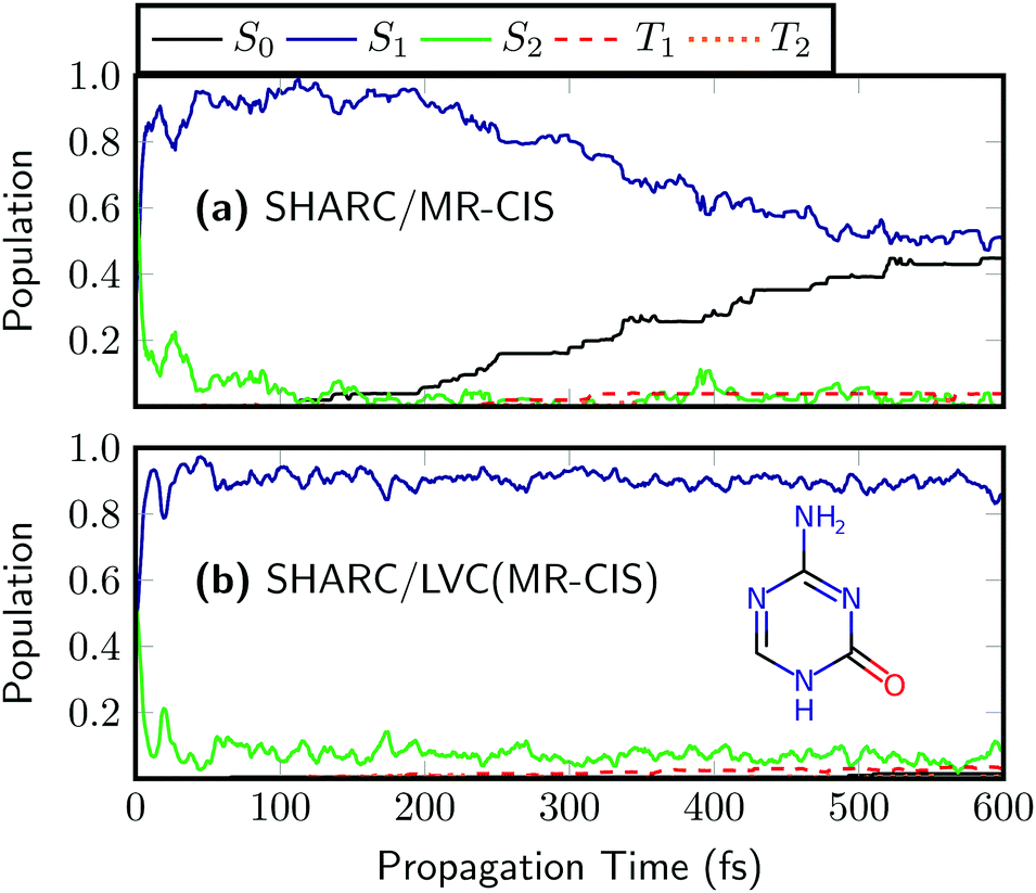
In a next step, the ultrafast dynamics after UV absorption are investigated for adenine and 2AP using the LVC(MR-CIS) model. The results for adenine are shown in Fig. 5(a). First, there is an ultrafast rise of the S1 state population, reaching a maximum value of 93% after 74 fs followed by a somewhat slower decay to S0. Both features, the initial rise of S1 and its subsequent decay agree remarkably well with on-the-fly MR-CIS dynamics, reported previously.52 A similar sub-100 fs process in the excited state manifold has also been observed with a quadratic coupling model in reduced dimensionality.96 The obtained relaxation time constants are 31 ± 2 fs and 1070 ± 100 fs for S2 → S1 and S1 → S0, respectively. These time constants agree very well with the experimental values of <100 fs and 700–1030 fs.50,51 At this point it is worth mentioning that the ultrafast nonradiative decay of adenine cannot be reproduced by time-dependent density functional theory (TDDFT) using a range of different popular density functionals.92,97 This shows that it is clearly a challenging feat to describe the process correctly and shows that an LVC model can even outperform on-the-fly TDDFT dynamics. While we do not claim that the SHARC/LVC protocol will always perform perfectly, it is fair to say that often it may be preferable to use an LVC model parameterized against a high-level reference instead of using a lower level method on-the-fly.
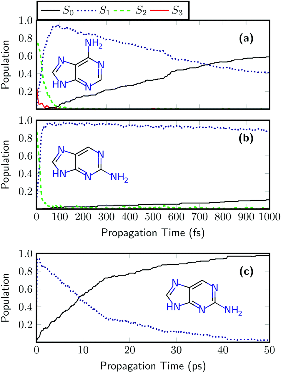 | ||
| Fig. 5 Time evolution of the adiabatic singlet state populations of (a) 9H-adenine and (b) 9H-2-aminopurine after photoexcitation computed using LVC surface hopping based on MR-CIS(10,8)/aug-cc-pVDZ potentials. In panel (c) the evolution until 50 ps is presented for 9H-2-aminopurine. | ||
It is especially interesting to study whether the LVC model can describe the geometrical displacements leading to the S1/S0 decay, which are characterized by strong out-of-plane distortions of the aromatic rings.52,53,97 To this end, we show in Fig. 6 four exemplary S1/S0 hopping geometries from the LVC(MR-CIS) simulations. Indeed, the LVC model can predict these strong out-of-plane deformations, even though the LVC model is expanded around the almost perfectly planar S0 minimum. This is primarily achieved through non-zero out-of-plane λ values between the diabatic 21nπ* and 21ππ* states. Consequently, at the hopping geometries the adiabatic S1 state is a linear combination of the 21nπ* and 21ππ* states, while the adiabatic S0 state is mostly of closed-shell character (with a weight >70%).
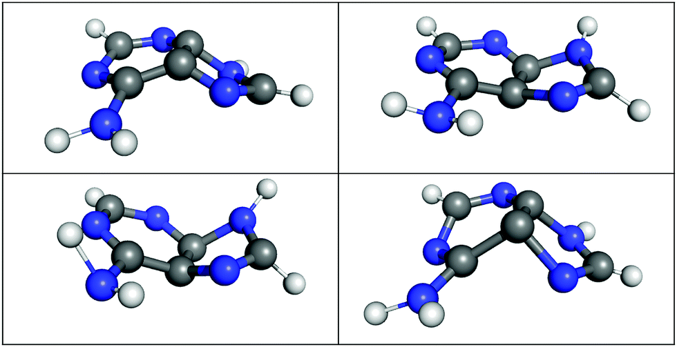 | ||
| Fig. 6 Selected S1/S0 hopping geometries as obtained during LVC(MR-CIS) surface hopping dynamics of adenine. | ||
The dynamics results for 2AP are presented in Fig. 5(b). Also in this case an ultrafast rise of S1 occurs, and an S1 population of 92% is reached after only 32 fs. When compared to adenine, the subsequent decay to the ground state is significantly slowed down and after 1 ps, a ground state population of only 10% is reached, highlighting the enhanced nonradiative lifetime of 2AP. From Fig. 5(b) alone, it is challenging to obtain an accurate estimate of the excited state lifetime. Therefore, the dynamics simulations were extended up to 50 ps. Such dynamics simulations, requiring over 16 million electronic structure computations for the whole ensemble, are far beyond the scope of ab initio on-the-fly dynamics but can be easily performed with the LVC model. The results, presented in Fig. 5(c), reveal that after 9.0 ps, 50% of the population has decayed to the ground state. The fitted time constants for 2AP are 17 ± 1 fs and 13000 ± 1000 fs for the S2 → S1 and S1 → S0 processes. The latter timescale is about one order of magnitude faster than the experimental value of 156 ps reported for jet-cooled 2AP.55 The main source for this error is probably the description of the low frequency out-of-plane modes. These are expected to experience non-negligible anharmonicities, which are not described in the LVC model. In order to definitely answer the question whether this problem is related to the LVC approximation, the level of theory MR-CIS, or the surface hopping protocol one would have to perform ab initio MR-CIS dynamics, which are unfortunately unfeasible for the required timescale. Nonetheless, the employed LVC model correctly predicts two important properties of gas phase 2AP: that its lifetime is significantly longer than the one of adenine, and that it nevertheless decays on a picosecond timescale.
3.3 2-Thiocytosine and 5-azacytosine
To investigate the more general applicability for the new protocol, we finish this work by briefly studying two modified nucleobases. As a first example, we study 2-thiocytosine, i.e., keto-cytosine where one of the oxygen atoms is replaced by sulfur. The on-the-fly results for 2TC are presented in Fig. 7(a).58 Using the employed excitation window the dynamics starts predominantly in the S2 state. S2 decays on a time scale of about 160 fs, and the population is transferred to the T1 and S1 states with minor contributions from T2 and S2. Ultrafast ISC occurs with a time constant of 250 fs.58 At the end of the simulated period, the dominant state is T1 with a population of 58% and a total triplet yield of 75% is obtained. The main features of the dynamics, i.e. the S2 decay and the ultrafast ISC are well-captured by the SHARC/LVC dynamics shown in Fig. 7(b). Similarly to SO2 the main difference is that SHARC/LVC somewhat underestimates the T1 population and the overall triplet yield, which is only 56% at the end of the simulated period. In general, the good performance of the LVC model for 2TC can be ascribed to the rigidity of the system in its excited state.58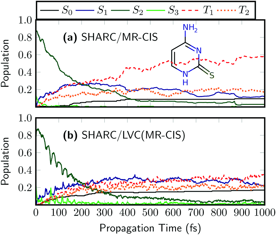 | ||
| Fig. 7 Time evolution of the adiabatic populations of 2-thiocytosine after photoexcitation computed at the (a) on-the-fly and (b) LVC levels in SHARC using MR-CIS(6,5)/cc-pVDZ. | ||
As a final example, we want to discuss the 5-azacytosine molecule. The on-the-fly results63 for 5AC are presented in Fig. 8(a). The initial excitation is distributed over the S2 and S1. A very rapid rise of S1 follows and after about 100 fs almost all the population is in S1. Around the same time, the rise of S0 starts and after 600 fs about half the population has transferred to S0. Triplet population is negligible. The SHARC/LVC dynamics [Fig. 8(b)] reproduces the initial ultrafast transfer to S1 and the absence of ISC in this system, and generally provides a good reproduction of the first 100 fs. However, it was not possible to reproduce the ultrafast decay to the ground state for 5AC. A likely reason for this behaviour is the presence of a barrier in the reaction path leading to the minimum energy conical intersection between S1 and S0.63 In order to reproduce this barrier correctly, it is probably necessary to move beyond the LVC model.
 | ||
| Fig. 8 Time evolution of the adiabatic populations of 5-azacytosine after photoexcitation computed at the (a) on-the-fly and (b) LVC levels in SHARC using MR-CIS(6,5)/cc-pVDZ. | ||
4 Conclusions
A new implementation of the LVC model was reported, amenable for performing nonadiabatic trajectory surface hopping simulations and for constructing post-Condon spectra using a Wigner distribution formalism requiring only minimal computational and human effort. Utilities were developed that allow a parameterization of the model from only a ground-state frequency computation and one excited-state single-point computation. It was shown that despite being a simple and blackbox approach the method provides a powerful tool for addressing a variety of photophysical as well as methodological questions.In the case of SO2, it was shown that the LVC model could reproduce all the features of the on-the-fly MR-CIS dynamics simulations while reducing the computational cost by about three orders of magnitude. It was also illustrated that the LVC model could be applied to evaluate the effects of the significantly enhanced MR-CISD level of electronic structure theory. Finally, because of the fact that the LVC model could be employed identically in quantum dynamics and surface hopping simulations, it provided a rigorous route for benchmarking the latter for realistic Hamiltonians of high-dimensional systems. Conversely, the method could, in the future, be used in the context of quantum dynamics studies, as it allows to efficiently evaluate the effect of neglecting different degrees of freedom.
An investigation of the prototypical adenine and 2AP molecules showed that the SHARC/LVC method allows to correctly discriminate between the different qualitative behavior of these two molecules: subpicosecond decay was found in the former whereas a significantly enhanced nonradiative lifetime was found in the latter. These results suggest that in cases where the LVC approximation is expected to work the method can be used as a blackbox and computationally cheap approach to evaluate whether or not a molecule is expected to be fluorescent – a notoriously difficult task in computational photochemistry.
Further tests were performed in 2TC and 5AC. In the case of 2TC, ultrafast decay of S2 and ISC was found in agreement with on-the-fly dynamics. For 5AC some qualitative features of the on-the-fly dynamics were reproduced but the SHARC/LVC protocol failed to describe ultrafast decay to the ground state. The case of 5AC serves as a reminder that the “one shot” LVC approach investigated here is only the lowest level of a hierarchy of possibilities to approximate on-the-fly dynamics and will not always provide a definite answer. Nonetheless, it is impressive that the correct qualitative behaviour was found in four out of the five molecules studied considering the simplicity and computational efficiency of the approach.
It was shown that SHARC/LVC allows for a speed up of about three orders of magnitude compared to on-the-fly dynamics. This means that one can study one thousand molecules instead of one, a nanosecond instead of a picosecond, or an ensemble of 100000 trajectories instead of 100 allowing to study even very rare processes. Due to this low computational cost and its ease of use, we expect the presented protocol to be a powerful addition to the currently available computational photochemistry toolbox. We believe that it is a significant advancement towards black-box nonadiabatic dynamics methods, which could find applications in high-throughput screening for different purposes, e.g., fluorescent dyes or photostable drug molecules. At the same time caution is certainly in place. The presented protocol arises from the dire need of performing ab initio photodynamics simulations without incurring excessive computational costs. Whenever on-the-fly dynamics simulations are feasible at the same electronic structure level these are to be preferred over LVC dynamics and if quantum dynamics are possible, these are to be preferred over LVC surface hopping. Conversely, the protocol presents an attractive option for cases where ab initio on-the-fly dynamics is too expensive or the number of degrees of freedom is too large for quantum dynamics. We have used a “one shot” LVC approach, where all excited-state data is obtained from a single electronic structure computation, to show that even this simplest approximation provides reasonable results, at least in cases where no strong structural rearrangement occurs. To improve the description, it is possible to move to more sophisticated vibronic coupling models, which are readily created using established protocols.26,28
For the purpose of advancing to larger, more complex systems it will be possible to use embedding methods, to proceed through interpolation of diabatic Hamiltonians19,20 or to incorporate exciton models in the dynamics.98–100
Conflicts of interest
There are no conflicts to declare.Acknowledgements
Funding from the University of Vienna and the Austrian Science Fund (FWF) within project I2883 is gratefully acknowledged. FP thanks Loughborough University for startup funding. The Vienna Scientific Cluster is thanked for computational support. MM gratefully acknowledges financial support from the EU Horizon 2020 research and innovation program under the Marie Skłodowska-Curie grant agreement no. 642294. The authors thank M. Fumanal, E. Gindensperger, C. Daniel, and G. A. Worth for discussions regarding the LVC model.References
- J. C. Tully, J. Chem. Phys., 1990, 93, 1061–1071 CrossRef CAS.
- D. Polli, P. Altoè, O. Weingart, K. M. Spillane, C. Manzoni, D. Brida, G. Tomasello, G. Orlandi, P. Kukura, R. A. Mathies, M. Garavelli and G. Cerullo, Nature, 2010, 467, 440–443 CrossRef CAS.
- M. Barbatti, A. J. A. Aquino, J. J. Szymczak, D. Nachtigallová, P. Hobza and H. Lischka, Proc. Natl. Acad. Sci. U. S. A., 2010, 107, 21453–21458 CrossRef CAS.
- S. Gozem, H. L. Luk, I. Schapiro and M. Olivucci, Chem. Rev., 2017, 117, 13502–13565 CrossRef CAS.
- G. Cui and W. Thiel, Angew. Chem., Int. Ed., 2013, 52, 433–436 CrossRef CAS.
- A. V. Akimov, A. J. Neukirch and O. V. Prezhdo, Chem. Rev., 2013, 113, 4496–4565 CrossRef CAS.
- M. Richter, P. Marquetand, J. Gonzalez-Vazquez, I. Sola and L. Gonzalez, J. Chem. Theory Comput., 2011, 7, 1253–1258 CrossRef CAS.
- S. Mai, M. Pollum, L. Martínez-Fernández, N. Dunn, P. Marquetand, I. Corral, C. E. Crespo-Hernández and L. González, Nat. Commun., 2016, 7, 13077 CrossRef CAS.
- C. Xu, L. Yu, C. Zhu, J. Yu and Z. Cao, Sci. Rep., 2016, 6, 26768 CrossRef CAS.
- J. P. Zobel, J. J. Nogueira and L. González, Chem. – Eur. J., 2018, 24, 5379–5387 CrossRef CAS.
- A. J. Atkins and L. González, J. Phys. Chem. Lett., 2017, 8, 3840–3845 CrossRef CAS.
- M. Barbatti, WIREs Comput. Mol. Sci., 2011, 1, 620 CrossRef CAS.
- T. Nelson, S. Fernandez-Alberti, A. E. Roitberg and S. Tretiak, Acc. Chem. Res., 2014, 47, 1155–1164 CrossRef CAS.
- L. Du and Z. Lan, J. Chem. Theory Comput., 2015, 11, 1360–1374 CrossRef CAS.
- S. Pal, D. J. Trivedi, A. V. Akimov, B. Aradi, T. Frauenheim and O. V. Prezhdo, J. Chem. Theory Comput., 2016, 12, 1436–1448 CrossRef CAS.
- J. E. Subotnik, A. Jain, B. Landry, A. Petit, W. Ouyang and N. Bellonzi, Annu. Rev. Phys. Chem., 2016, 67, 387–417 CrossRef CAS.
- S. Mai, P. Marquetand and L. González, WIREs Comput. Mol. Sci., 2018, e1370 CrossRef.
- R. Crespo-Otero and M. Barbatti, Chem. Rev., 2018, 118, 7026–7068 CrossRef CAS PubMed.
- J. W. Park and Y. M. Rhee, J. Chem. Theory Comput., 2014, 10, 5238–5253 CrossRef CAS PubMed.
- J. W. Park and Y. M. Rhee, J. Chem. Phys., 2014, 140, 164112 CrossRef PubMed.
- J. Ischtwan and M. A. Collins, J. Chem. Phys., 1994, 100, 8080–8088 CrossRef CAS.
- G. W. Richings, I. Polyak, K. E. Spinlove, G. A. Worth, I. Burghardt and B. Lasorne, Int. Rev. Phys. Chem., 2015, 34, 269–308 Search PubMed.
- J. Behler and M. Parrinello, Phys. Rev. Lett., 2007, 98, 146401 CrossRef.
- M. Gastegger, J. Behler and P. Marquetand, Chem. Sci., 2017, 8, 6924–6935 RSC.
- H. Köppel, W. Domcke and L. S. Cederbaum, Adv. Chem. Phys., 1984, 57, 59–246 Search PubMed.
- H. Köppel, J. Gronki and S. Mahapatra, J. Chem. Phys., 2001, 115, 2377–2388 CrossRef.
- M. Fumanal and C. Daniel, J. Comput. Chem., 2016, 3, 2454–2466 CrossRef.
- C. Cattarius, A. Markmann and G. A. Worth, The VCHAM program, 2007, see http://www.pci.uni-heidelberg.de/tc/usr/mctdh/doc.85/vcham/index.html Search PubMed.
- G. A. Worth and L. S. Cederbaum, Annu. Rev. Phys. Chem., 2004, 55, 127–158 CrossRef CAS.
- M. H. Beck, A. Jäckle, G. A. Worth and H.-D. Meyer, Phys. Rep., 2000, 324, 1–105 CrossRef CAS.
- A. Raab, G. A. Worth, H.-D. Meyer and L. S. Cederbaum, J. Chem. Phys., 1999, 110, 936–946 CrossRef CAS.
- R. P. Krawczyk, K. Malsch, G. Hohlneicher, R. C. Gillen and W. Domcke, Chem. Phys. Lett., 2000, 320, 535–541 CrossRef CAS.
- S. Faraji, H.-D. Meyer and H. Köppel, J. Chem. Phys., 2008, 129, 074311 CrossRef.
- C. Lévêque, A. Komainda, R. Taïeb and H. Köppel, J. Chem. Phys., 2013, 138, 044320 CrossRef.
- G. A. Worth, G. Welch and M. J. Paterson, Mol. Phys., 2006, 104, 1095–1105 CrossRef CAS.
- J. Eng, C. Gourlaouen, E. Gindensperger and C. Daniel, Acc. Chem. Res., 2015, 48, 809–817 CrossRef CAS.
- H. Tamura and I. Burghardt, J. Am. Chem. Soc., 2013, 135, 16364–16367 CrossRef CAS.
- U. Müller and G. Stock, J. Chem. Phys., 1997, 107, 6230–6245 CrossRef.
- S. Mai, P. Marquetand and L. González, Int. J. Quantum Chem., 2015, 115, 1215–1231 CrossRef CAS.
- S. Mai, M. Richter, M. Heindl, M. F. S. J. Menger, A. Atkins, M. Ruckenbauer, F. Plasser, M. Oppel, P. Marquetand and L. González, Sharc2.0: Surface Hopping Including Arbitrary Couplings – Program Package for Non-Adiabatic Dynamics, 2018, available from http://sharc-md.org Search PubMed.
- C. Xie, X. Hu, L. Zhou, D. Xie and H. Guo, J. Chem. Phys., 2013, 139, 014305 CrossRef.
- I. Wilkinson, A. E. Boguslavskiy, J. Mikosch, J. B. Bertrand, H. J. Wörner, D. M. Villeneuve, M. Spanner, S. Patchkovskii and A. Stolow, J. Chem. Phys., 2014, 140, 204301 CrossRef.
- S. Mai, P. Marquetand and L. González, J. Chem. Phys., 2014, 140, 204302 CrossRef.
- C. Lévêque, R. Taïeb and H. Köppel, J. Chem. Phys., 2014, 140, 091101 CrossRef PubMed.
- C. Lévêque, D. Peláez, H. Köppel and R. Taïeb, Nat. Commun., 2014, 5, 4126 CrossRef.
- F. Franco de Carvalho and I. Tavernelli, J. Chem. Phys., 2015, 143, 224105 CrossRef CAS.
- J. Heicklen, N. Kelly and K. Partymiller, Res. Chem. Intermed., 1980, 3, 315–404 CrossRef CAS.
- C. R. Guest, R. A. Hochstrasser, L. C. Sowers and D. P. Millar, Biochemistry, 1991, 30, 3271–3279 CrossRef CAS.
- L. Serrano-Andres, M. Merchan and A. C. Borin, Proc. Natl. Acad. Sci. U. S. A., 2006, 103, 8691–8696 CrossRef CAS.
- S. Ullrich, T. Schultz, M. Z. Zgierski and A. Stolow, Phys. Chem. Chem. Phys., 2004, 6, 2796 RSC.
- N. L. Evans and S. Ullrich, J. Phys. Chem. A, 2010, 114, 11225–11230 CrossRef CAS.
- M. Barbatti and H. Lischka, J. Am. Chem. Soc., 2008, 130, 6831–6839 CrossRef CAS.
- E. Fabiano and W. Thiel, J. Phys. Chem. A, 2008, 112, 6859–6863 CrossRef CAS.
- A. N. Alexandrova, J. C. Tully and G. Granucci, J. Phys. Chem. B, 2010, 114, 12116–12128 CrossRef CAS.
- S. Lobsiger, S. Blaser, R. K. Sinha, H. M. Frey and S. Leutwyler, Nat. Chem., 2014, 6, 989–993 CrossRef CAS.
- T. Fiebig, C. Wan and A. H. Zewail, ChemPhysChem, 2002, 3, 781–788 CrossRef CAS.
- M. Pollum, L. Martínez-Fernández and C. E. Crespo-Hernández, in Photochemistry of Nucleic Acid Bases and Their Thio- and Aza-Analogues in Solution, ed. M. Barbatti, A. C. Borin and S. Ullrich, Springer International Publishing, Cham, 2015, pp. 245–327 Search PubMed.
- S. Mai, M. Pollum, L. Martínez-Fernández, N. Dunn, P. Marquetand, I. Corral, C. E. Crespo-Hernández and L. González, Nat. Commun., 2016, 7, 1–8 Search PubMed.
- D. Koyama, M. J. Milner and A. J. Orr-Ewing, J. Phys. Chem. B, 2017, 121, 9274–9280 CrossRef CAS.
- S. Bai and M. Barbatti, Phys. Chem. Chem. Phys., 2017, 19, 12674–12682 RSC.
- J. H. Saiki, K. B. McCredie, T. J. Vietti, J. S. Hewlett, F. S. Morrison, J. J. Costanzi, W. J. Stuckey, J. Whitecar and B. Hoogstraten, Cancer, 1978, 42, 2111–2114 CrossRef CAS.
- T. Kobayashi, H. Kuramochi, Y. Harada, T. Suzuki and T. Ichimura, J. Phys. Chem. A, 2009, 113, 12088–12093 CrossRef CAS.
- A. C. Borin, S. Mai, P. Marquetand and L. González, Phys. Chem. Chem. Phys., 2017, 19, 5888–5894 RSC.
- S. Mai, F. Plasser, P. Marquetand and L. González, Attosecond Molecular Dynamics, The Royal Society of Chemistry, 2019 Search PubMed.
- M. Fumanal, F. Plasser, S. Mai, C. Daniel and E. Gindensperger, J. Chem. Phys., 2018, 148, 124119 CrossRef.
- M. S. Schuurman and D. R. Yarkony, J. Chem. Phys., 2007, 127, 094104 CrossRef.
- H. Lischka, M. Dallos, P. G. Szalay, D. R. Yarkony and R. Shepard, J. Chem. Phys., 2004, 120, 7322–7329 CrossRef CAS.
- T. Ichino, J. Gauss and J. F. Stanton, J. Chem. Phys., 2009, 130, 174105 CrossRef.
- A. Tajti and P. G. Szalay, J. Chem. Phys., 2009, 131, 124104 CrossRef.
- F. Plasser, M. Ruckenbauer, S. Mai, M. Oppel, P. Marquetand and L. González, J. Chem. Theory Comput., 2016, 12, 1207 CrossRef CAS.
- G. Granucci, M. Persico and A. Toniolo, J. Chem. Phys., 2001, 114, 10608–10615 CrossRef CAS.
- G. Granucci, M. Persico and A. Zoccante, J. Chem. Phys., 2010, 133, 134111 CrossRef.
- F. Plasser, G. Granucci, J. Pittner, M. Barbatti, M. Persico and H. Lischka, J. Chem. Phys., 2012, 137, 22A514 CrossRef.
- P. G. Szalay, T. Muller, G. Gidofalvi, H. Lischka and R. Shepard, Chem. Rev., 2012, 112, 108 CrossRef CAS.
- B. O. Roos, R. Lindh, P.-Å. Malmqvist, V. Veryazov and P.-O. Widmark, J. Phys. Chem. A, 2004, 108, 2851–2858 CrossRef CAS.
- M. Reiher, Theor. Chem. Acc., 2006, 116, 241–252 Search PubMed.
- B. A. Heß, C. M. Marian, U. Wahlgren and O. Gropen, Chem. Phys. Lett., 1996, 251, 365–371 CrossRef.
- P. Å. Malmqvist, B. O. Roos and B. Schimmelpfennig, Chem. Phys. Lett., 2002, 357, 230–240 CrossRef CAS.
- S. Mai, T. Müller, F. Plasser, P. Marquetand, H. Lischka and L. González, J. Chem. Phys., 2014, 141, 074105 CrossRef.
- H. Lischka, M. Dallos and R. Shepard, Mol. Phys., 2002, 100, 1647–1658 CrossRef CAS.
- R. A. Kendall, T. H. Dunning Jr. and R. J. Harrison, J. Chem. Phys., 1992, 96, 6796 CrossRef CAS.
- H. Lischka, R. Shepard, R. M. Pitzer, I. Shavitt, M. Dallos, T. Muller, P. G. Szalay, M. Seth, G. S. Kedziora, S. Yabushita and Z. Y. Zhang, Phys. Chem. Chem. Phys., 2001, 3, 664–673 RSC.
- H. Lischka, T. Müller, P. G. Szalay, I. Shavitt, R. M. Pitzer and R. Shepard, Wiley Interdiscip. Rev.: Comput. Mol. Sci., 2011, 1, 191–199 CAS.
- H. Lischka, R. Shepard, I. Shavitt, R. M. Pitzer, M. Dallos, T. Muller, P. G. Szalay, F. B. Brown, R. Ahlrichs, H. J. Boehm, A. Chang, D. C. Comeau, R. Gdanitz, H. Dachsel, C. Ehrhardt, M. Ernzerhof, P. Hoechtl, S. Irle, G. Kedziora, T. Kovar, V. Parasuk, M. J. M. Pepper, P. Scharf, H. Schiffer, M. Schindler, M. Schueler, M. Seth, E. A. Stahlberg, J.-G. Zhao, S. Yabushita, Z. Zhang, M. Barbatti, S. Matsika, M. Schuurmann, D. R. Yarkony, S. R. Brozell, E. V. Beck, J.-P. Blaudeau, M. Ruckenbauer, B. Sellner, F. Plasser, R. F. K. Szymczak, J. J. Spada and A. Das, COLUMBUS: An Ab Initio Electronic Structure Program, Release 7.0, http://www.univie.ac.at/columbus, 2017 Search PubMed.
- F. Aquilante, et al. , J. Comput. Chem., 2016, 37, 506–541 CrossRef CAS.
- T. Helgaker, H. J. A. Jensen, P. Jorgensen, J. Olsen, K. Ruud, H. Agren, T. Andersen, K. L. Bak, V. Bakken, O. Christiansen, P. Dahle, E. K. Dalskov, T. Enevoldsen, H. Heiberg, H. Hettema, D. Jonsson, S. Kirpekar, R. Kobayashi, H. Koch, K. V. Mikkelsen, P. Norman, M. J. Packer, T. Saue, P. R. Taylor and O. Vahtras, DALTON, an ab initio electronic structure program, release 1.0, 1997 Search PubMed.
- J. P. Dahl and M. Springborg, J. Chem. Phys., 1988, 88, 4535–4547 CrossRef CAS.
- TURBOMOLE V7.0.1 2017, a development of University of Karlsruhe and Forschungszentrum Karlsruhe GmbH, 1989–2007, TURBOMOLE GmbH, since 2007, available from http://www.turbomole.com Search PubMed.
- S. Nangia, A. W. Jasper, T. F. Miller and D. G. Truhlar, J. Chem. Phys., 2004, 120, 3586–3597 CrossRef CAS.
- D. Golomb, K. Watanabe and F. F. Marmo, J. Chem. Phys., 1962, 36, 958–960 CrossRef CAS.
- J. Bloino, M. Biczysko, F. Santoro and V. Barone, J. Chem. Theory Comput., 2010, 6, 1256–1274 CrossRef CAS.
- M. Barbatti, Z. Lan, R. Crespo-Otero, J. J. Szymczak, H. Lischka and W. Thiel, J. Chem. Phys., 2012, 137, 22A503 CrossRef.
- C. Plützer, E. Nir, M. S. de Vries and K. Kleinermanns, Phys. Chem. Chem. Phys., 2001, 3, 5466–5469 RSC.
- A. Holmén, B. Nordén and B. Albinsson, J. Am. Chem. Soc., 1997, 119, 3114–3121 CrossRef.
- K. A. Seefeld, C. Plützer, D. Löwenich, T. Häber, R. Linder, K. Kleinermanns, J. Tatchen and C. M. Marian, Phys. Chem. Chem. Phys., 2005, 7, 3021 RSC.
- D. Picconi, F. J. Avila Ferrer, R. Improta, A. Lami and F. Santoro, Faraday Discuss., 2013, 163, 223 RSC.
- F. Plasser, R. Crespo-Otero, M. Pederzoli, J. Pittner, H. Lischka and M. Barbatti, J. Chem. Theory Comput., 2014, 10, 1395–1405 CrossRef CAS.
- R. Binder, J. Wahl, S. Römer and I. Burghardt, Faraday Discuss., 2013, 163, 205 RSC.
- A. Sisto, C. Stross, M. W. van der Kamp, M. O'Connor, S. McIntosh-Smith, G. T. Johnson, E. G. Hohenstein, F. R. Manby, D. R. Glowacki and T. J. Martinez, Phys. Chem. Chem. Phys., 2017, 19, 14924–14936 RSC.
- S. Jurinovich, L. Cupellini, C. A. Guido and B. Mennucci, J. Comput. Chem., 2018, 39, 279–286 CrossRef CAS.
Footnote |
| † Electronic supplementary information (ESI) available: Employed LVC parameters for SO2 (S1–S4) and details on the fitting procedures for Ade and 2AP (S5) (pdf); SHARC input files containing all LVC parameters and data underlying the presented figures (zip). See DOI: 10.1039/c8cp05662e |
| This journal is © the Owner Societies 2019 |