Multiscale virtual particle based elastic network model (MVP-ENM) for normal mode analysis of large-sized biomolecules
Kelin
Xia

Division of Mathematical Sciences, School of Physical and Mathematical Sciences, Nanyang Technological University, Singapore 637371. E-mail: xiakelin@ntu.edu.sg; Tel: +65 6513 7464
First published on 1st December 2017
Abstract
In this paper, a multiscale virtual particle based elastic network model (MVP-ENM) is proposed for the normal mode analysis of large-sized biomolecules. The multiscale virtual particle (MVP) model is proposed for the discretization of biomolecular density data. With this model, large-sized biomolecular structures can be coarse-grained into virtual particles such that a balance between model accuracy and computational cost can be achieved. An elastic network is constructed by assuming “connections” between virtual particles. The connection is described by a special harmonic potential function, which considers the influence from both the mass distributions and distance relations of the virtual particles. Two independent models, i.e., the multiscale virtual particle based Gaussian network model (MVP-GNM) and the multiscale virtual particle based anisotropic network model (MVP-ANM), are proposed. It has been found that in the Debye–Waller factor (B-factor) prediction, the results from our MVP-GNM with a high resolution are as good as the ones from GNM. Even with low resolutions, our MVP-GNM can still capture the global behavior of the B-factor very well with mismatches predominantly from the regions with large B-factor values. Further, it has been demonstrated that the low-frequency eigenmodes from our MVP-ANM are highly consistent with the ones from ANM even with very low resolutions and a coarse grid. Finally, the great advantage of MVP-ANM model for large-sized biomolecules has been demonstrated by using two poliovirus virus structures. The paper ends with a conclusion.
1 Introduction
It is well known that structure flexibility and dynamic motions are of essential importance to biomolecular functions. Experimentally, biomolecular flexibility can be directly or indirectly observed from X-ray crystallography, nuclear magnetic resonance (NMR) and single-molecule force experiments.1 The experimental measurement, called Debye–Waller factors (also known as B-factors or temperature factors), is widely-used to quantitatively characterize the biomolecular flexibility. Computationally, molecular dynamics (MD)2 has proven to be one of the most powerful tools for analyzing not only biomolecular flexibility, but also biomolecular conformational changes. MD has been widely used in biophysics and structure biology. However, even with the ever-increasing computational powers, MD may still fail to simulate the dynamics, particularly the long-timescale dynamics, of macromolecules or biomolecular complexes. Therefore, alternative approaches, including normal mode analysis (NMA),3–6 graph theory7 and the elastic network model (ENM)8–15 have been proposed. Among these methods, NMA is a rather old technique used in mechanical dynamical systems from physics and engineering. Its recent popularity in biomolecular structure analysis is due to the observation that for biomolecules, particularly macroproteins or protein complexes, one or a few low-frequency normal modes are able to capture their global movements,14,16 which are usually functionally relevant.14,16 The essential idea of NMA is to use a harmonic function to approximate the potential energy function near an equilibrium state. In this way, biomolecular motions can be decomposed into a series of vibrational modes. And the global motions are approximated by one or a few low-frequency eigenmodes. Further, Tirion17 simplifies the potential energy function in NMA by using pseudo-harmonic functions between any atoms within a cutoff distance. This results in the so-called elastic network model (ENM).11,17 ENM can dramatically reduce the computational time due to two major reasons. First, no energy minimization is required as the crystal structure is regarded as the energy minima state. Second, various coarse-grained representations are used in ENM. The two most popular models in ENM are Gaussian network model (GNM)8,9 and anisotropic network model (ANM).10 GNM is proposed to describe isotropic positional fluctuations. It is highly accurate and efficient in B-factor prediction.18–20 ANM is often used in the normal mode analysis of biomolecules.Two major challenges exist in biomolecular flexibility and normal mode analysis. The first one comes from extremely large biomolecular complexes.21–26 To reduce the biomolecular complexity, coarse-graining (CG) techniques are usually considered. In the past two decades, based on CG techniques, various approaches have been proposed, including rotation-translation of blocks (RTB),27 the block normal mode (BNM) algorithm,13,28 molecular symmetry based NMA,29 essential dynamics coarse-graining (ED-CG),15,30,31 the NMA based fluctuation matching method (NMA-FM),32–34 the iterative matrix projection method35etc. In RTB and BNM, several residues are consolidated into a single residue block. Rigid-body motions of these residual blocks provide the low-frequency normal modes. In molecular symmetry based NMA, the Cartesian basis is replaced by a symmetry coordinate basis. This new basis includes only internal dihedral angles thus significantly reducing the degrees of freedom for symmetric structures. In the ED-CG model, a coarse-grained model is determined by preserving the essential functional motions of a biomolecule. These motions can be obtained from principal component analysis (PCA) of MD simulation trajectories or the eigenmodes in ENM. ED-CG is based on the heterogeneous ENM,15 whose parameters are directly derived from MD simulation. In the NMA-FM method, a coarse-grained model is uniquely designed so that the physical properties, particularly fluctuations, predicted by this CG model and the original all-atom model are consistent. The potential function used in NMA-FM is constructed by using some effective internal coordinates. Finally, in the iterative matrix projection method, the Hessian matrix from the all-atom representation is rewritten as the combination of a coarse-grained part and a residual part. An iterative projection is then used to generate a coarse-grained Hessian matrix, which can still capture the dynamics of the all-atom model very well. The iterative matrix projection method is derived from its previous spring-based NMA and simplified spring-based NMA models.36
The other challenge comes from analyzing the dynamics of biomolecular structures in density data, particularly the ones obtained from cryo-electron microscopy (Cryo-EM).37,38 Due to experimental limitations, a great amount of cryo-EM data, particularly for large biomolecular structures, are in low resolution. The detailed atomic information cannot be deciphered from the data. Therefore, analyzing the flexibility and dynamics of these biomolecular structures is by no means trivial. The quantized elastic deformation model (QEDM)39–42 was one of the first methods proposed for analyzing the normal modes of cryo-EM data. It has been found that biomolecular conformational changes or collective global motions are largely determined by their global shapes and mass distributions.39,41,43,44 Therefore, in QEDM, biomolecules are treated as elastic objects and the vector quantization (VQ) algorithm45 is used to discretize them into a set of Voronoi cells.37,46 QEDM has been successfully used in B-factor and collective motion prediction. Another method for Cryo-EM data analysis is the bend-twist-stretch (BTS) model. It was developed for coarse-graining biomolecular structures into networks by shifting the spatial complexity into potential functions.47 The BTS model also employs VQ for the discretization of cryo-EM data. The competitive Hebb rule48 is used to establish connections between adjacent pseudo-atoms, which are centroids of Voronoi cells. In this way, pseudo-bonds and pseudo-angles can be defined and a BTS model is constructed. The potential function in the BTS model has contributions from not only bonds, but also bond angles and dihedral angles, and all parameters are derived from continuum mechanics models. The ED-CG model30 stated above can also be used in Cryo-EM data analysis. Similar to QEDM and BTS, the VQ method is also used in discretization.
In this paper, a multiscale virtual particle based elastic network model (MVP-ENM) is introduced for the normal mode analysis of large-sized biomolecules. The basic ideas in MVP-ENM can be traced back to the flexibility–rigidity index (FRI).20,49 FRI has been proven to be a highly accurate and efficient method for biomolecular flexibility analysis. Free from eigenvalue decomposition, the computational complexity of FRI is ![[scr O, script letter O]](https://www.rsc.org/images/entities/char_e52e.gif) (N2) with N as the total number of Cα atoms. The fast FRI (fFRI)20 employs the cell list algorithm50 and is of
(N2) with N as the total number of Cα atoms. The fast FRI (fFRI)20 employs the cell list algorithm50 and is of ![[scr O, script letter O]](https://www.rsc.org/images/entities/char_e52e.gif) (N) complexity only. For the HIV virus capsid with 313
(N) complexity only. For the HIV virus capsid with 313![[thin space (1/6-em)]](https://www.rsc.org/images/entities/char_2009.gif) 236 residues, fFRI is able to predict its B-factors in less than 30 seconds on a single-core processor.20 However, FRI and fFRI can only be used in isotropic fluctuation analysis. Even though the anisotropic FRI (aFRI) can be used in normal mode prediction, it still requires eigenvalue decomposition and has the same computational limitations as ANM. To solve this problem and further develop a new aFRI model for Cryo-EM data analysis, a virtual particle based aFRI model (VP-aFRI) is proposed.51 In the VP-aFRI model, virtual particles are elements from the discretization of the density distribution. They are “connected” with each other through harmonic functions, whose spring constants are determined by the relative distance and mass distributions of the VPs. The VP-aFRI model has been successfully used in the normal mode analysis of Cryo-EM data.51
236 residues, fFRI is able to predict its B-factors in less than 30 seconds on a single-core processor.20 However, FRI and fFRI can only be used in isotropic fluctuation analysis. Even though the anisotropic FRI (aFRI) can be used in normal mode prediction, it still requires eigenvalue decomposition and has the same computational limitations as ANM. To solve this problem and further develop a new aFRI model for Cryo-EM data analysis, a virtual particle based aFRI model (VP-aFRI) is proposed.51 In the VP-aFRI model, virtual particles are elements from the discretization of the density distribution. They are “connected” with each other through harmonic functions, whose spring constants are determined by the relative distance and mass distributions of the VPs. The VP-aFRI model has been successfully used in the normal mode analysis of Cryo-EM data.51
Similar to the previous VP-aFRI model,51 MVP-ENM is designed based on biomolecular density data. In the MVP model, the discretization can be done in different ways. The Cartesian grid as in the finite difference method, the tetrahedron mesh as in the finite element method, the Voronoi cell as in the tessalation method, etc. can all be employed in the discretization of the computational domain. More importantly, depending on the available computational resources and the properties of the biomolecular density data, we choose a suitable mesh that has a relatively small size but can still capture the general shape of the structure. After that, an elastic network is constructed by connecting the virtual elements with “springs”. This spring parameter has incorporated in it the geometry and mass distribution information of the virtual particles. Finally, an eigenvalue decomposition of either the Laplacian matrix or Hessian matrix is employed. B-Factors and collective modes are then evaluated from the eigenvalues and eigenvectors. To facilitate a comparison between the predictions and experimental results, we interpolate the prediction values, which are calculated on virtual particles, onto the atoms. This is done by using a nearest neighbour scheme.
The paper is organized as follows. Section 2 is devoted to the multiscale virtual particle based elastic network model, including its basic setting, modeling and algorithm. Results and discussions can be found in Section 3. The paper ends with a conclusion.
2 Models and methods
One of the major features of biological sciences in the 21st century is its transition from an empirical, qualitative and phenomenological discipline to a comprehensive, quantitative and predictive one. A tremendous amount of biomolecular structural data are available in the Protein Data Bank (PDB) and the Electron Microscopy Data Bank (EMDB). The analysis of the dynamics of these structures is essential to the understanding of the function and mechanism of these biomolecules. Traditional approaches, including molecular dynamics, normal model analysis, elastic network models, etc., have been widely used in biomolecular motion analysis and yielded fruitful results. However, with the availability of more large-sized macroproteins and biomolecular complexes, the computational limitations of these approaches have begun to reveal themselves. Moreover, the rapid advance in cryo-electron microscopy has enabled researchers to generate structural data of extremely large-sized biomolecular complexes and assemblies in their native environment. However, traditional approaches, which can only be applied to structures with atomic details, fail in the dynamic analysis of cryo-EM data.In this section, a multiscale virtual particle model based elastic network model is proposed to analyze the collective motion of large-sized biomolecules. MVP-ENM is based on elastic network models and the multiscale virtual particle model. It is constructed on the molecular density function, therefore it can be directly applied to Cryo-EM data analysis. Details of the models are presented in the following.
2.1 Elastic network models
Due to its great simplicity and efficiency, the elastic network model has been widely used in biomolecular flexibility and normal mode analysis.10,11,17 The Gaussian network model8,9,13,14,52 and the anisotropic network model10,11 are the two most commonly used ENMs. Since MVP-ENM is based on elastic network models, GNM and ANM are briefly reviewed. | (1) |
 | (2) |
 | (3) |
 Here, L−1 is the Moore–Penrose pseudo-inverse of the Laplacian matrix L. More specifically,
  , where T denotes the transpose and λk and vk are the k-th eigenvalue and eigenvector of L, respectively. The summation omits the first eigenmode, as its eigenvalue is zero. The predicted i-th B-factor by GNM8,9,19 can be expressed as
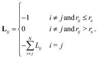
  . The cutoff distance rc is usually chosen between 7 Å to 15 Å18,53 Yang et al.18 point out that GNM is about one order more efficient than most other flexibility approaches. However, GNM is an isotropic model and cannot provide molecular motions. To explore the collective dynamics of biomolecules, ANM was proposed.
 | (4) |
 | (5) |
 The equilibrium correlation between fluctuations is
  . Again, H−1 is the pseudo-inverse matrix. More specifically,
  where T denotes the transpose. And λk and vk are the k-th eigenvalue and eigenvector of H, respectively. The summation omits the first six eigenmodes, whose eigenvalues are zero. Further, the predicted i-th B-factor8,9,19 can be expressed as
  . ANM has been proven to be a powerful tool for normal mode analysis. Due to its great efficiency, it has been successfully applied to macroproteins and protein complexes, such as ribosomes,22,23 virus capsid,24,25 chaperonin GroEL,26etc. Various software and online solvers have been designed for this.16 A more detailed discussion can be found in recent review papers.14,18
2.2 Multiscale virtual particle (MVP) model
Biomolecular data are usually highly complicated and essentially multiscale. Our previous works on multiscale models have indicated that a better representation of the multiscale biomolecular structure can improve the accuracy of the models in flexibility analysis.54–56 Further, based on the density representation, a multiscale virtual particle model is proposed to model the network structure from different scales.51 | (6) |
| Φ(‖r − rj‖;η,κ) = e−(‖r−rj/η)κ, κ > 0, | (7) |
A multiscale geometric model can be naturally derived from the multiscale rigidity function. By tuning the scale resolution value, the geometric model can capture structural properties from different scales. To further facilitate the comparison between different scales, a normalized density function is proposed as follows,
 | (8) |
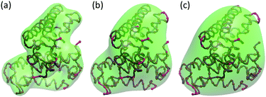 | ||
| Fig. 1 Biomolecular surfaces of Protein 2CCY from three different scales. The molecular density data are generated by using the generalized Gaussian model in eqn (7) with κ = 2 and three different resolution values, i.e., η = 5 Å, 10 Å and 15 Å. The density data are normalized using eqn (8). Biomolecular surfaces are generated with the isovalue 0.4. | ||
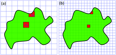
The most critical piece of the MVP model is to find suitable “connections” between VPs. Since VPs vary greatly in their shapes, sizes and mass-distributions, an identical spring constant as in traditional ENMs will no longer be suitable. Therefore, we propose a spring parameter that is determined by VP properties.63 To facilitate the presentation, we still consider the biomolecule in Fig. 2 as an example. We assume that its normalized density distribution is μs(r). The spring parameter between the two VPs with domains ΩI and ΩJ can be expressed as follows,
| γIJ = γ(rI,rJ,ΩI,ΩJ,μs(r),ηMVP) = γ1(ΩI,ΩJ,μs(r))·γ2(rI,rJ,ηMVP) | (9) |
Here, rI and rJ are centers of the I-th and J-th virtual particle. Parameter γ1(ΩI,ΩJ,μs(r)) is the part of the spring parameter that considers the mass or density contribution. Parameter γ2(rI,rJ,ηMVP) is the other part of the spring parameter that considers the distance influence. The resolution parameter ηMVP is related to the scale of the MVP model. To avoid confusion with the previous scale resolution η, we call ηMVP the spatial resolution.
For the density contribution part, since the spring parameter between two virtual particles is positively related to their total density, virtual particles with a large total density will have a large spring constant. With this consideration, γ1(ΩI,ΩJ,μs(r)) can be modeled as,
 | (10) |
For the distance contribution part, a distance related function is considered in the MVP model. Traditional elastic network models usually employ a cutoff distance. Atoms within this cutoff distance are connected by a uniformed spring value. In the MVP model, the cutoff distance is replaced by a soft kernel. Essentially, the distance related parameter γ2(rI,rJ,ηMVP) can be chosen from generalized Gaussian kernels as in eqn (7). For example,
| γ2(rI,rJ,ηMVP) = e−(‖rI−rJ‖/ηMVP)κ, κ > 0. | (11) |
In this paper, the Cartesian grid is used in domain discretization for simplicity. All regular VPs are defined on grid boxes with a uniform size. The ΩI illustrated in Fig. 2 is a typical domain of a regular VP. However, some VPs near the boundary may have irregular shapes such as ΩJ in Fig. 2. In this situation, we simply approximate all irregular VPs with regular VPs. For example, an irregular VP defined on domain ΩJ will be replaced with a regular VP defined on the entire grid box, which includes the part of the grid box outside the protein domain. Further, to calculate γ1(ΩI,ΩJ,μs(r)), the integration term  is evaluated by a density value defined on the VP center,
 | (12) |
 . We can use the same approximation and have
  . Finally, all the VP centers, such as rI and rJ, are chosen to be on the Cartesian grid points. With all these approximations, the MVP model can be easily implemented.
With these basic settings, we are ready to introduce MVP-ENM, which includes two different models, i.e., a multiscale virtual particle based Gaussian network model (MVP-GNM) and a multiscale virtual particle based anisotropic network model (MVP-ANM).
2.3 Multiscale virtual particle based elastic network model (MVP-ENM)
As stated in the introduction, a pronounced weakness of the traditional NMA, ENM, and ANM is that they cannot be used in Cryo-EM data analysis.39 To overcome this problem, the quantized elastic deformation model is proposed. In this method, the vector quantization algorithm45 is employed to decompose the electron density map of a biological molecule into a set of finite Voronoi cells. It is then combined with ANM to explore the dynamics of the cryo-EM data.39,41 Two other models, i.e., the bend-twist-stretch (BTS) model47 and ED-CG model,30 have also been modified to handle cryo-EM data. A common feature of these models is that they all employ VQ to do the discretization and rely on Voronoi cells to construct the network model. MVP-ENM uses various discretization approaches, particularly the Cartesian grid, thus it is free from the computational complexity of VQ. In this section, we discuss the details of MVP-ENM. | (13) |
 | (14) |
 | (15) |
Again, γIJ = γ(rI,rJ,ΩI,ΩJ,μs(r),ηMVP) is the spring parameter between virtual particles at rI and rJ. The diagonal element is the negative summation of the off-diagonal elements in the same row,
MVP-ANM can be used in B-factor prediction. The formulae remain the same as the ones in Section 2.1.2. More importantly, MVP-ANM can be directly used in the normal mode analysis of Cryo-EM data.
3 Results and discussion
This section is devoted to the validation of MVP-ENM. We first compare MVP-GNM with GNM in B-factor prediction. We find that the results from density data with high scale resolution are as good as the GNM predictions. This shows that MVP-ENM characterizes the biomolecular intrinsic connectivity information very well. Then, we compare MVP-ANM with ANM in normal mode prediction and find that the prediction of the low-frequency eigenmodes from MVP-ANM is highly consistent with ANM results, which again confirms that MVP-ANM is well-designed and highly reliable. Finally, we discuss the application of MVP-ANM in the analysis of large-sized biomolecules, particularly the ones from Cryo-EM data. We have shown that MVP-ANM is able to overcome the computational limitation of traditional normal mode methods.3.1 MVP-GNM for B-factor prediction
We choose three proteins with IDs 2ABH, 2CCY and 1AQB to validate MVP-GNM. Protein 2ABH was previously used in the anisotropic flexibility–rigidity index model.20 The other two proteins are test cases from QEDM.39 The molecular density data are generated by using the generalized Gaussian model in eqn (7) with κ = 2. We use three different scale resolution values, i.e., η = 5 Å, 10 Å and 15 Å, to generate molecular density data in three different scales. An example of the 2CCY density data can be found in Fig. 1. In discretization schemes, the Cartesian grid is employed with a grid spacing 2.0 Å. The computational domain is chosen as the region or regions with normalized density values larger than or equal to 0.4, i.e., μs(r;η) ≥ 0.4. In GNM, the cutoff distance is chosen as 7 Å. For the spring parameter γ1(ΩI,ΩJ,μs(r)), the approximation formula in eqn (12) is used. For γ2(rI,rJ,ηMVP), the generalized Gaussian kernel as in eqn (11) is used. The parameter κ is chosen as 2 and the spatial resolution ηMVP is chosen as the same value as the scale resolution η.The predicted B-factors from GNM and MVP-GNM are illustrated in Fig. 3–5. The Pearson correlation coefficients (PCCs) between the experimental and the predicted B-factors are listed in Table 1. It can be seen that the prediction from MVP-GNM with the finest scale resolution (η = 5 Å) is almost as good as the ones from GNM. Even for the lowest resolutions, MVP-GNM can still preserve the basic patterns or global shapes of the original B-factor profiles. Further, the mismatches or wrongly-predicted domains are mostly from the regions with extremely large B-factors. This means that MVP-GNM characterizes the global behaviors or properties of the structure very well. Our predictions are comparable with the results from QEDM.39 It is worth mentioning that due to the multiscale properties of biomolecules, it is not always true that a high PCC can be obtained from a higher scale resolution.54,55 Essentially, our scale parameter can be roughly understood as a soft kernel approximation of the cutoff distance. And the best cutoff distance can vary between different proteins.
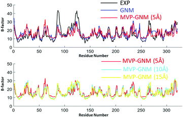 | ||
| Fig. 3 Comparison of B-factor prediction with GNM and MVP-GNM for protein 2ABH. In MVP-GNM, three different scale values, i.e., η = 5 Å, 10 Å and 15 Å, are used to generate protein density data in different scale resolutions. It can be seen that for data in all three scale resolutions, MVP-GNM is able to capture the basic global pattern of the B-factors very well. The PCC for GNM is 0.647, and the PCCs for MVP-GNM with η = 5 Å, 10 Å and 15 Å are 0.634, 0.741 and 0.796, respectively. The extremely high PCC at the lowest scale resolution may due to the multiscale properties of protein 2ABH. | ||
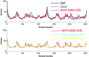 | ||
| Fig. 4 Comparison of B-factor prediction with GNM and MVP-GNM for protein 2CCY. Again, three different scale values, i.e., η = 5 Å, 10 Å and 15 Å, are used to generate the protein density data in MVP-GNM. It can be seen that for data in all three scale resolutions, MVP-GNM is able to capture the basic global pattern of the B-factors very well. The PCC for GNM is 0.739, and the PCCs for MVP-GNM with η = 5 Å, 10 Å and 15 Å are 0.737, 0.583 and 0.484, respectively. | ||
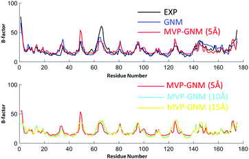 | ||
| Fig. 5 Comparison of B-factor prediction with GNM and MVP-GNM for protein 1AQB. Similar to the previous two examples, three different scale values, i.e., η = 5 Å, 10 Å and 15 Å, are used to generate protein density data in MVP-GNM. Similarly, we can find that for data in all three resolutions, MVP-GNM is able to capture the basic global pattern of the B-factors very well. The PCC for GNM is 0.822, and the PCCs for MVP-GNM with η = 5 Å, 10 Å and 15 Å are 0.742, 0.722 and 0.770, respectively. | ||
3.2 MVP-ANM for normal mode analysis
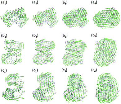
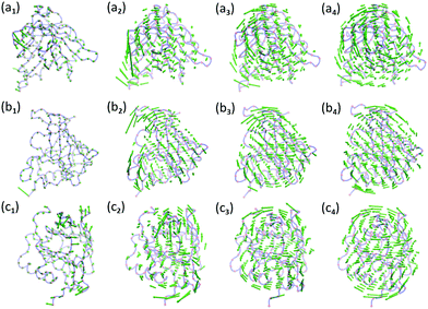
We only consider three nontrivial lowest-frequency eigenmodes. They correspond to the eigenvectors 7 to 9, as the first six eigenvalues are zero. The results are illustrated in Fig. 6–8. Subfigures (a), (b) and (c) represent the eigenmodes 7 to 9, respectively. Subscript 1 is for ANM results. Subscripts 2 to 4 represent the results from the scale resolution values η = 5 Å, 10 Å and 15 Å, respectively. For instance, subfigure (a3) is for eigenmode 8 from MVP-ANM with the resolution value η = 10 Å. It can be seen that for proteins 2ABH and 2CCY, the eigenmodes predicted by MVP-ANM and ANM have highly consistent rotation directions and patterns. To obtain a more quantitative comparison, we decompose each eigenmode into three individual vectors with X-direction components, Y-direction components and Z-direction components from this eigenmode separately, and then interpolate the results from virtual particles onto atoms. Further, the PCCs between ANM and MVP-ANM are calculated. We only consider the lowest resolution situation (η = 15 Å), and list the mean PCC value, the average of the X, Y and Z results, in Table 2. It can be seen that relatively good PCCs are obtained for all the three eigenmodes.
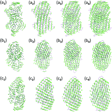 | ||
| Fig. 6 The comparison of the three nontrivial lowest-frequency eigenmodes from ANM and MVP-ANM for protein 2ABH. The indexes a, b and c represent eigenmodes 7 to 9, respectively. Subscript 1 is for ANM results. Subscripts 2 to 4 are for MVP-ANM results using η = 5 Å, 10 Å and 15 Å, respectively. The normalized density data are used and the biomolecular domain is generated by using the isovalue 0.4. It can be seen that the predicted eigenvectors from MVP-ANM in three different resolutions are all highly consistent with ANM results. This demonstrates the robustness and consistency of MVP-ANM. | ||
 | ||
| Fig. 7 The comparison of the three nontrivial lowest-frequency eigenmodes from ANM and MVP-ANM for protein 2CCY. The indexes a, b and c represent eigenmodes 7 to 9, respectively. Subscript 1 is for ANM results. Subscripts 2 to 4 are for MVP-ANM results using η = 5 Å, 10 Å and 15 Å, respectively. The normalized density data are used and the biomolecular domain is generated by using the isovalue 0.4. Again, we can see that the eigenvectors from MVP-ANM in three different resolutions are all highly consistent with ANM results. This further demonstrates the robustness and consistency of MVP-ANM. | ||
 | ||
| Fig. 8 The comparison of the three nontrivial lowest-frequency eigenmodes from MVP-ANM for protein 1AQB. The subfigure notations are the same as those in Fig. 6 and 7. In this case, the eigenmodes from ANM are irregular and have one or several extremely large local 3 by 1 vectors. In MVP-ANM, by increasing the scale resolution value to 10 Å and 15 Å, we smooth out some local details and the global motions can be captured by the lowest-frequency eigenmodes very well. Moreover, the eigenmodes from scale resolutions of 10 Å and 15 Å are highly consistent. | ||
We notice that for protein 1AQB, its eigenmodes from ANM are highly irregular. As illustrated in Fig. 8, one or several local eigenvectors (3 by 1) have a disproportionately large value and overshadow all the other local vectors. These large values are usually from regions with extruding loops or ends. Since our multiscale density representation has a controllable scale resolution parameter, we can enlarge its value to systematically remove these local details and attenuate their contributions to the low-frequency eigenmodes. As demonstrated in Fig. 8, when the scale resolution value increases, the amplitude of these irregular local eigenvectors reduces dramatically and global motions begin to emerge. More interestingly, there is a clear consistency of the eigenmodes from MVP-ANM with the resolutions σ = 10 Å and 15 Å.
From the above analysis, it can be seen that MVP-ANM is able to preserve the basic collective motions even at very low resolutions with a very coarse grid. Our results are consistent with the finding39,40,43 that the collective motions are highly related to the global shapes and mass distributions, and insensitive to local structure variations.
We use protein 2ABH as an example. Its density data are generated with the resolution η = 10 Å. We choose several different isovalues and compare the three lowest nontrivial eigenmodes. The results are demonstrated in Fig. 9. Subfigures (a), (b) and (c) are for eigenmodes 7 to 9, respectively. The results of two different isovalues, i.e., 0.6 and 0.8, are illustrated on the left and right hand side of each subfigure, respectively. Even though the total numbers of virtual particles from these two isovalues differ greatly, it can be seen that the normal modes from the two isovalue models share similar rotation directions and patterns. And they are consistent with ANM results in Fig. 6. More interestingly, when the isovalue equals 0.4, there are 372 virtual particles in total. This number drops to 195 when the isovalue equals 0.6 and further plummets to 77 if isovalue 0.8 is used. However, even with the dramatic reduction of virtual particles, the general pattern of the collective motions still remains the same.
From the above analysis, it can be seen that MVP-ANM is relatively robust over a certain range of isovalues. This is because when a coarse resolution is used, the general shapes from these isovalues are relatively consistent. Therefore, the pattern of the collective motions remains the same. More importantly, this means that in the virtual particle generation, MVP-ANM can have certain flexibility in the selection of isovalues.
In the first case, the virus structure from the PDB is represented as point cloud data with each point representing an atom. To coarse-grain this large virus structure, we transfer it from point cloud data into density data. Similar to previous cases, the generalized Gaussian model as in eqn (7) is used with κ = 2. The resolution parameter and the grid spacing are all chosen as 4 Å to ensure enough structure details are preserved. The protein surface is generated by using isovalue 0.13. In the MVP model, if we define each voxel (or grid box) with a density value larger or equal to 0.1 as a virtual particle, the size of the Hessian matrix will be too large to be computationally affordable. To avoid that, we combine the adjacent five voxels in each direction together into a single virtual particle. In this way, each virtual particle has a total of 125 voxels from the density data. The scale parameter in the spring constant is chosen as the size of the virtual particle, which is 20 Å. With this setting, there are only 1008 virtual particles in the MVP-ANM model and the Hessian matrix is 3024 × 3024. In the original ANM, even in the coarse-grained representation, the virus 1XYR still has 43![[thin space (1/6-em)]](https://www.rsc.org/images/entities/char_2009.gif) 440 Cα atoms and its Hessian matrix is 130
440 Cα atoms and its Hessian matrix is 130![[thin space (1/6-em)]](https://www.rsc.org/images/entities/char_2009.gif) 320 × 130
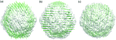
320 × 130![[thin space (1/6-em)]](https://www.rsc.org/images/entities/char_2009.gif) 320. The reduction of the computational cost is dramatic. More interestingly, the low-frequency normal modes are well-preserved in our model. Fig. 10 illustrates the three types of lowest-frequency normal modes from MVP-ANM. Due to the structural symmetry, each type of normal mode represents several eigenvectors with the same global motion but different orientations. Roughly speaking, the first mode is to compress in the middle region and expand on the top and bottom. The second mode is to compress on the bottom, expand on the top and rotate in the middle. The third mode is to rotate counterclockwise on the top half-sphere and clockwise on the bottom half-sphere. These three types of motions are widely observed in the poliovirus virus.29 They are tightly related to the icosahedron structure of the virus.
320. The reduction of the computational cost is dramatic. More interestingly, the low-frequency normal modes are well-preserved in our model. Fig. 10 illustrates the three types of lowest-frequency normal modes from MVP-ANM. Due to the structural symmetry, each type of normal mode represents several eigenvectors with the same global motion but different orientations. Roughly speaking, the first mode is to compress in the middle region and expand on the top and bottom. The second mode is to compress on the bottom, expand on the top and rotate in the middle. The third mode is to rotate counterclockwise on the top half-sphere and clockwise on the bottom half-sphere. These three types of motions are widely observed in the poliovirus virus.29 They are tightly related to the icosahedron structure of the virus.
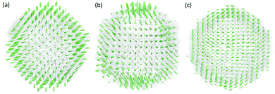 | ||
Fig. 10 The illustration of the three types of nontrivial lowest-frequency eigenmodes of the poliovirus structure with ID 1XYR. The virus structure has 43![[thin space (1/6-em)]](https://www.rsc.org/images/entities/char_2009.gif) 440 Cα atoms, which are coarse-grained into 1008 virtual particles in the MVP-ANM model. The three types of lowest-frequency eigenmodes from MVP-ANM are widely observed in the poliovirus virus structure. 440 Cα atoms, which are coarse-grained into 1008 virtual particles in the MVP-ANM model. The three types of lowest-frequency eigenmodes from MVP-ANM are widely observed in the poliovirus virus structure. | ||
In the second example, the virus structure is represented in density data. These density data have 201 × 201 × 201 voxels and the size of each voxel is 2.322 Å × 2.322 Å × 2.322 Å. We consider the virus surface generated with isovalue 10. In the MVP model, if each voxel with density values larger than 10 is treated as an individual virtual particle, this again will result in a huge number of virtual particles beyond the computational limit. Therefore, we combine the adjacent 8 voxels in each direction together into a single virtual particle. With this setting, there are 1267 virtual particles. Again, this process reduces the computational complexity tremendously. The result is depicted in Fig. 11. We do not list all the possible eigenmodes. Instead three types of the lowest nontrivial eigenmodes are considered. By the comparison of the results in Fig. 10 and 11, it can be observed that the two structures share almost identical types of collective motions. This is not a surprise, as both have a rather regular icosahedron symmetry structure. Different scales of the virtual particle model are also employed, and there is great consistency in these types of collective motions. The results again confirm that biomolecular collective motions are directly related to their general shape.
4 Conclusion
A multiscale virtual particle based elastic network model (MVP-ENM) is proposed for the normal mode analysis of large-sized biomolecules. Two independent models, i.e., the multiscale virtual particle based Gaussian network model (MVP-GNM) and the multiscale virtual particle based anisotropic network model (MVP-ANM), are included in MVP-ENM. It is found that with a high scale resolution, MVP-GNM is able to predict the Debye–Waller factors with considerably good accuracy. The mismatches are predominantly from higher fluctuation regions. Further, MVP-ANM delivers very consistent low-frequency eigenmodes even for density data with very low resolutions and coarse grids. Our model can greatly reduce computational complexity.Conflicts of interest
There are no conflicts to declare.Acknowledgements
This work was supported in part by the Nanyang Technological University Startup Grant M408110000 and the Singapore Ministry of Education Academic Research fund Tier 1 M401110000.References
- O. K. Dudko, G. Hummer and A. Szabo, Intrinsic rates and activation free energies from single-molecule pulling experiments, Phys. Rev. Lett., 2006, 96, 108101 CrossRef PubMed.
- J. A. McCammon, B. R. Gelin and M. Karplus, Dynamics of folded proteins, Nature, 1977, 267, 585–590 CrossRef CAS PubMed.
- N. Go, T. Noguti and T. Nishikawa, Dynamics of a small globular protein in terms of low-frequency vibrational modes, Proc. Natl. Acad. Sci. U. S. A., 1983, 80, 3696–3700 CrossRef CAS.
- M. Tasumi, H. Takenchi, S. Ataka, A. M. Dwidedi and S. Krimm, Normal vibrations of proteins: Glucagon, Biopolymers, 1982, 21, 711–714 CrossRef CAS PubMed.
- B. R. Brooks, R. E. Bruccoleri, B. D. Olafson, D. J. States, S. Swaminathan and M. Karplus, Charmm: A program for macromolecular energy, minimization, and dynamics calculations, J. Comput. Chem., 1983, 4, 187–217 CrossRef CAS.
- M. Levitt, C. Sander and P. S. Stern, Protein normal-mode dynamics: Trypsin inhibitor, crambin, ribonuclease and lysozyme, J. Mol. Biol., 1985, 181(3), 423–447 CrossRef CAS PubMed.
- D. J. Jacobs, A. J. Rader, L. A. Kuhn and M. F. Thorpe, Protein flexibility predictions using graph theory, Proteins: Struct., Funct., Genet., 2001, 44(2), 150–165 CrossRef CAS PubMed.
- I. Bahar, A. R. Atilgan and B. Erman, Direct evaluation of thermal fluctuations in proteins using a single-parameter harmonic potential, Folding Des., 1997, 2, 173–181 CrossRef CAS PubMed.
- I. Bahar, A. R. Atilgan, M. C. Demirel and B. Erman, Vibrational dynamics of proteins: Significance of slow and fast modes in relation to function and stability, Phys. Rev. Lett., 1998, 80, 2733–2736 CrossRef CAS.
- A. R. Atilgan, S. R. Durrell, R. L. Jernigan, M. C. Demirel, O. Keskin and I. Bahar, Anisotropy of fluctuation dynamics of proteins with an elastic network model, Biophys. J., 2001, 80, 505–515 CrossRef CAS PubMed.
- K. Hinsen, Analysis of domain motions by approximate normal mode calculations, Proteins, 1998, 33, 417–429 CrossRef CAS.
- F. Tama and Y. H. Sanejouand, Conformational change of proteins arising from normal mode calculations, Protein Eng., 2001, 14, 1–6 CrossRef CAS PubMed.
- G. H. Li and Q. Cui, A coarse-grained normal mode approach for macromolecules: an efficient implementation and application to Ca(2+)-ATPase, Biophys. J., 2002, 83, 2457–2474 CrossRef CAS PubMed.
- Q. Cui and I. Bahar, Normal mode analysis: theory and applications to biological and chemical systems, Chapman and Hall/CRC, 2010 Search PubMed.
- E. Lyman, J. Pfaendtner and G. A. Voth, Systematic multiscale parameterization of heterogeneous elastic network models of proteins, Biophys. J., 2008, 95(9), 4183–4192 CrossRef CAS PubMed.
- L. Skjaerven, S. M. Hollup and N. Reuter, Normal mode analysis for proteins, J. Mol. Struct., 2009, 898, 42–48 CrossRef CAS.
- M. M. Tirion, Large amplitude elastic motions in proteins from a single-parameter, atomic analysis, Phys. Rev. Lett., 1996, 77, 1905–1908 CrossRef CAS PubMed.
- L. W. Yang and C. P. Chng, Coarse-grained models reveal functional dynamics–I. elastic network models–theories, comparisons and perspectives, Bioinf. Biol. Insights, 2008, 2, 25–45 CAS.
- J. K. Park, Robert Jernigan and Z. Wu, Coarse grained normal mode analysis vs. refined gaussian network model for protein residue-level structural fluctuations, Bull. Math. Biol., 2013, 75, 124–160 CrossRef CAS PubMed.
- K. Opron, K. L. Xia and G. W. Wei, Fast and anisotropic flexibility–rigidity index for protein flexibility and fluctuation analysis, J. Chem. Phys., 2014, 140, 234105 CrossRef PubMed.
- O. Keskin, I. Bahar, D. Flatow, D. G. Covell and R. L. Jernigan, Molecular mechanisms of chaperonin groel-groes function, Biochem., 2002, 41, 491–501 CrossRef CAS.
- F. Tama, M. Valle, J. Frank and C. K. Brooks III, Dynamic reorganization of the functionally active ribosome explored by normal mode analysis and cryo-electron microscopy, Proc. Natl. Acad. Sci. U. S. A., 2003, 100(16), 9319–9323 CrossRef CAS PubMed.
- Y. Wang, A. J. Rader, I. Bahar and R. L. Jernigan, Global ribosome motions revealed with elastic network model, J. Struct. Biol., 2004, 147, 302–314 CrossRef CAS PubMed.
- A. J. Rader, D. H. Vlad and I. Bahar, Maturation dynamics of bacteriophage hk97 capsid, Structure, 2005, 13, 413–421 CrossRef CAS PubMed.
- F. Tama and C. K. Brooks III, Diversity and identity of mechanical properties of icosahedral viral capsids studied with elastic network normal mode analysis, J. Mol. Biol., 2005, 345, 299–314 CrossRef CAS PubMed.
- W. Zheng, B. R. Brooks and D. Thirumalai, Allosteric transitions in the chaperonin groel are captured by a dominant normal mode that is most robust to sequence variations, Biophys. J., 2007, 93, 2289–2299 CrossRef CAS PubMed.
- P. Durand, G. Trinquier and Y. H. Sanejouand, A new approach for determining low-frequency normal modes in macromolecules, Biopolymers, 1994, 34(6), 759–771 CrossRef CAS.
- F. Tama, F. X. Gadea, O. Marques and Y. H. Sanejouand, Building-block approach for determining low-frequency normal modes of macromolecules, Proteins: Struct., Funct., Bioinf., 2000, 41(1), 1–7 CrossRef CAS.
- W. T. Herman, V. van and M. Karplus, Normal mode calculations of icosahedral viruses with full dihedral flexibility by use of molecular symmetry, J. Mol. Biol., 2005, 350(3), 528–542 CrossRef PubMed.
- Z. Zhang and G. A. Voth, Coarse-grained representations of large biomolecular complexes from low-resolution structural data, J. Chem. Theory Comput., 2010, 6(9), 2990–3002 CrossRef CAS PubMed.
- Z. Zhang, L. Lu, W. G. Noid, V. Krishna, J. Pfaendtner and G. A. Voth, A systematic methodology for defining coarse-grained sites in large biomolecules, Biophys. J., 2008, 95(11), 5073–5083 CrossRef CAS PubMed.
- J. W. Chu and G. A. Voth, Allostery of actin filaments: molecular dynamics simulations and coarse-grained analysis, Proc. Natl. Acad. Sci. U. S. A., 2005, 102(37), 13111–13116 CrossRef CAS PubMed.
- J. W. Chu and G. A. Voth, Coarse-grained modeling of the actin filament derived from atomistic-scale simulations, Biophys. J., 2006, 90(5), 1572–1582 CrossRef CAS PubMed.
- F. Xia and L. Y. Lu, Multiscale coarse-graining via normal mode analysis, J. Chem. Theory Comput., 2012, 8(11), 4797–4806 CrossRef CAS PubMed.
- H. Na, R. L. Jernigan and G. Song, Bridging between NMA and elastic network models: preserving all-atom accuracy in coarse-grained models, PLoS Comput. Biol., 2015, 11(10), e1004542 Search PubMed.
- H. Na and G. Song, Bridging between normal mode analysis and elastic network models, Proteins: Struct., Funct., Bioinf., 2014, 82(9), 2157–2168 CrossRef CAS PubMed.
- W. Wriggers, R. A. Milligan and J. A. McCammon, Situs: A package for docking crystal structures into low-resolution maps from electron microscopy, J. Struct. Biol., 1999, 125, 185–195 CrossRef CAS PubMed.
- W. Kühlbrandt, Cryo-em enters a new era, eLife, 2014, 3, 1–4 CrossRef PubMed.
- D. M. Ming, Y. F. Kong, M. A. Lambert, Z. Huang and J. P. Ma, How to describe protein motion without amino acid sequence and atomic coordinates, Proc. Natl. Acad. Sci. U. S. A., 2002, 99(13), 8620–8625 CrossRef CAS PubMed.
- D. M. Ming, Y. F. Kong, S. J. Wakil, J. Brink and J. P. Ma, Domain movements in human fatty acid synthase by quantized elastic deformational model, Proc. Natl. Acad. Sci. U. S. A., 2002, 99(12), 7895–7899 CrossRef CAS PubMed.
- F. Tama, W. Wriggers and C. L. Brooks, Exploring global distortions of biological macromolecules and assemblies from low-resolution structural information and elastic network theory, J. Mol. Biol., 2002, 321(2), 297–305 CrossRef CAS PubMed.
- P. Chacón, F. Tama and W. Wriggers, Mega-Dalton biomolecular motion captured from electron microscopy reconstructions, J. Mol. Biol., 2003, 326(2), 485–492 CrossRef.
- M. Y. Lu and J. P. Ma, The role of shape in determining molecular motions, Biophys. J., 2005, 89(4), 2395–2401 CrossRef CAS PubMed.
- F. Tama and C. L. Brooks III, Symmetry, form, and shape: guiding principles for robustness in macromolecular machines, Annu. Rev. Biophys. Biomol. Struct., 2006, 35, 115–133 CrossRef CAS PubMed.
- R. Gray, Vector quantization, IEEE ASSP Mag., 1984, 1(2), 4–29 CrossRef.
- W. Wriggers, R. A. Milligan, K. Schulten and J. A. McCammon, Self-organizing neural networks bridge the biomolecular resolution gap, J. Mol. Biol., 1998, 284(5), 1247–1254 CrossRef CAS PubMed.
- J. N. Stember and W. Wriggers, Bend-twist-stretch model for coarse elastic network simulation of biomolecular motion, J. Chem. Phys., 2009, 131(7), 074112 CrossRef PubMed.
- T. M. Martinetz, S. G. Berkovich and K. J. Schulten, ‘Neural-gas’ network for vector quantization and its application to time-series prediction, IEEE Trans. Neural Networks, 1993, 4(4), 558–569 CrossRef CAS PubMed.
- K. L. Xia, K. Opron and G. W. Wei, Multiscale multiphysics and multidomain models – Flexibility and Rigidity, J. Chem. Phys., 2013, 139, 194109 CrossRef PubMed.
- M. P. Allen and D. J. Tildesley, Computer Simulation of Liquids, Clarendon Press, Oxford, 1987 Search PubMed.
- K. L. Xia and G. W. Wei, A review of geometric, topological and graph theory apparatuses for the modeling and analysis of biomolecular data, 2016, arXiv preprint arXiv:1612.01735.
- L.-W. Yang, A. Rader, X. Liu, C. Jursa, S. Chen, H. Karimi and I. Bahar, oGNM: online computation of structural dynamics using the gaussian network model, Nucleic Acids Res., 2006, 34(Web Server issue), W24–W31 CrossRef CAS PubMed.
- S. Kundu, J. S. Melton, D. C. Sorensen and G. N. Phillips Jr., Dynamics of proteins in crystals: comparison of experiment with simple models, Biophys. J., 2002, 83, 723–732 CrossRef CAS PubMed.
- K. Opron, K. L. Xia and G. W. Wei, Communication: Capturing protein multiscale thermal fluctuations, J. Chem. Phys., 2015, 142(21), 211101 CrossRef PubMed.
- K. L. Xia, K. Opron and G. W. Wei, Multiscale Gaussian network model (mGNM) and multiscale anisotropic network model (mANM), J. Chem. Phys., 2015, 143(20), 204106 CrossRef PubMed.
- D. Nguyen, K. L. Xia and G. W. Wei, Generalized flexibility–rigidity index, J. Chem. Phys., 2016, 144(23), 234106 CrossRef PubMed.
- Pascal Jean Frey and P. L. George, Mesh generation: application to finite elements, 2000 Search PubMed.
- F. Labelle and J. R. Shewchuk. Isosurface stuffing: fast tetrahedral meshes with good dihedral angles. ACM Trans. Graph., 26(3), 2007 Search PubMed.
- H. Si, Constrained delaunay tetrahedral mesh generation and refinement, Finite Elem. Anal. Des., 2010, 46, 33–46 CrossRef.
- J. Tournois, C. Wormser, P. Alliez and M. Desbrun, Interleaving delaunay refinement and optimization for practical isotropic tetrahedron mesh generation, ACM Trans. Graph., 2009, 28(3), 75:1–75:9 CrossRef.
- Z. Y. Yu, M. Holst, Y. Cheng and J. A. McCammon, Feature-preserving adaptive mesh generation for molecular shape modeling and simulation, J. Mol. Graph. Model., 2008, 26, 1370–1380 CrossRef CAS PubMed.
- Xin Feng, Kelin Xia, Yiying Tong and Guo-Wei Wei, Geometric modeling of subcellular structures, organelles and large multiprotein complexes, Int. J. Numer. Meth. Bio. Eng., 2012, 28, 1198–1223 CrossRef PubMed.
- K. L. Xia, Z. M. Li and L. Mu, Multiscale persistent functions for biomolecular structure characterization, Bull. Math. Biol., 2017 DOI:10.1007/s11538-017-0362-6.
| This journal is © the Owner Societies 2018 |

