
 Open Access Article
 This Open Access Article is licensed under a
 Creative Commons Attribution 3.0 Unported Licence
Inertial migration and axial control of deformable capsules
Christian
Schaaf
 * and
Holger
Stark
* and
Holger
Stark
Institute of Theoretical Physics, Technical University Berlin, Hardenbergstr. 36, 10623 Berlin, Germany. E-mail: Christian.Schaaf@tu-berlin.de
First published on 26th April 2017
Abstract
The mechanical deformability of single cells is an important indicator for various diseases such as cancer, blood diseases and inflammation. Lab-on-a-chip devices allow to separate such cells from healthy cells using hydrodynamic forces. We perform hydrodynamic simulations based on the lattice-Boltzmann method and study the behavior of an elastic capsule in a microfluidic channel flow in the inertial regime. While inertial lift forces drive the capsule away from the channel center, its deformability favors migration in the opposite direction. Balancing both migration mechanisms, a deformable capsule assembles at a specific equilibrium distance depending on its size and deformability. We find that this equilibrium distance is nearly independent of the channel Reynolds number and falls on a single master curve when plotted versus the Laplace number. We identify a similar master curve for varying particle radius. In contrast, the actual deformation of a capsule strongly depends on the Reynolds number. The lift-force profiles behave in a similar manner as those for rigid particles. Using the Saffman effect, the capsule's equilibrium position can be controlled by an external force along the channel axis. While rigid particles move to the center when slowed down, very soft capsules show the opposite behavior. Interestingly, for a specific control force particles are focused on the same equilibrium position independent of their deformability.
1 Introduction
The mechanical deformability of biological cells is a sensitive quantity for identifying various diseases.1 Tumor cells, for example, are much softer than healthy cells,2,3 while malaria-infected red blood cells become much stiffer when occupied by the parasite.4,5 Microfluidic lab-on-a-chip devices utilize hydrodynamic effects in order to separate and probe biological cell samples.6–9 Such lab-on-a-chip devices are easy to use and can be designed as mass product. They are thus a helpful tool for especially improving medical conditions in poor countries.10The dynamics of deformable particles such as vesicles,11 capsules,12,13 or red blood cells14,15 has mostly been studied at low Reynolds numbers. Deformable particles migrate towards regions of low shear gradient. Thus, when immersed in a Poiseuille flow they move towards the channel center.16
At medium Reynolds numbers Segré and Silberberg observed that rigid particles in Poiseuille flow assemble in an annulus roughly half way between the center and the wall of a channel with circular cross section.17,18 Thus, in the non-uniform flow profile an inertial lift force occurs that initiates a drift motion directed away from the channel center. At the equilibrium distance this force is compensated by repulsive particle–wall interaction. The Segré–Silberberg effect is well studied in experiments,19–21 in theory using matched asymptotics,22,23 and in simulations.24,25 While the original setup used a cylindrical channel, microfluidic experiments are usually conducted with quadratic or rectangular channels, as they are easier to manufacture. Due to the reduced symmetry, the circular annulus is replaced by eight off-centered equilibrium positions in case of a quadratic channel (four on the main axes and four on the diagonals) or two on the short axes of a rectangular channel.26,27
In recent years also the dynamics of deformable particles in the inertial regime has been studied.28–33 In particular, Hur et al.34 demonstrated with their experiments that particles can be separated from each other based on their elastic deformability. Indeed, particles move closer to the channel center the softer and also the larger they are. This effect was also studied in simulations.35,36 Although all results agree that soft particles move to the channel center, the influence of the Reynolds number is not completely clear. While in some cases the final equilibrium distance from the channel center seems to depend on the Reynolds number,37,38 Kilimnik et al.35 found no evidence of such a behavior in their computer simulations. In contrast, they showed that the recorded values of the equilibrium distance collapse on a single master curve when plotted against the deformability of the particles.
Using additional control forces along the channel axis allows for further adjustment of the particles' equilibrium positions. In their experiments Kim and Yoo39 demonstrated that particles can be focused by applying an axial control force. They used an electric field to slow down the particles relative to the fluid. Due to the induced Saffman force, the particles migrated towards the channel center.40 While these experiments were performed at small Reynolds numbers, previous simulation work at moderate Reynolds numbers27 showed how an axial control force can move a rigid particle against the inertial lift force to a new equilibrium position. This position sensitively depends on the strength of the control force and the particle radius. Finally, the inertial focusing of particles can also be influenced by controlling their rotational motion41 or by designing external force fields with the help of optimal control theory.42
In this article we study the dynamics of a single deformable elastic capsule flowing through a microchannel with quadratic cross section. To simulate the Newtonian fluid, we employ the lattice-Boltzmann method together with the immersed boundary method. In the first part we study in detail the equilibrium positions of the elastic capsules, their deformations in the inertial Poiseuille flow, as well as the scaling of the lift-force profile by varying Reynolds number, particle rigidity, and radius. In an intermediate regime of particle rigidity, we confirm that the equilibrium distance hardly depends on Reynolds number and also identify a similar master curve for varying particle radius. The lift-force profiles behave in a similar manner as those for rigid particles.
In the second part we apply an external axial force to allow for an additional control of the equilibrium position. Extending the study of rigid particles in ref. 27, we find that a speed-up of the particle first induces a drift further away from the channel center, which then reverses for even stronger speed-up. This effect becomes more pronounced as the particles are softer. For very soft particles the behavior is opposite to rigid particles. A strong speed-up pushes them to the channel center while they move away from the center when slowed down. Interestingly, for a specific external control force all particles assemble at the same equilibrium distance independent of their deformability.
The article is organized as follows. In Section 2 we explain the set-up of our system, some details of the lattice-Boltzmann method, how we model deformable capsules, and the measurement of the lift-force profiles. In Section 3 we present the results including the detailed study of the equilibrium position, the deformations of the capsules, the lift-force profiles, and finally the influence of an external control force. We summarize and close with final remarks in Section 4.
2 Methods
2.1 Microfluidic setup in the simulations
We study a single deformable elastic capsule flowing in a microfluidic channel with a quadratic cross section (edge length 2w and channel length L; see Fig. 1). The pressure-driven Poiseuille flow points along the z direction and the origin of the coordinate system is in the channel center. The channel is filled with a Newtonian fluid with density ρ and kinematic viscosity ν. A constant local body force (see Section 2.2) generates the almost parabolic Poiseuille flow of a square channel.43 It is characterized by the channel Reynolds number Re = 2wumax/ν, where umax is the maximal flow velocity in the channel center.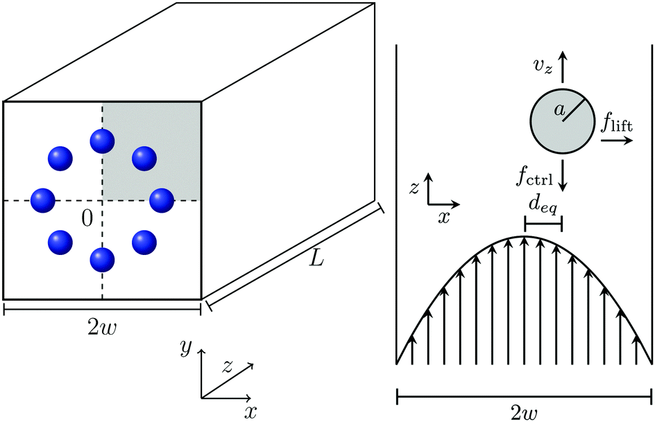 | ||
| Fig. 1 Left: Schematic of the microfluidic setup in the simulations. We use a quadratic channel with edge length 2w and channel length L. The channel center is located at x,y = 0. Due to the symmetry of the quadratic cross section, only the shaded area needs to be considered. The blue spheres indicate possible stable equilibrium positions. Right: Poiseuille flow in the xz plane. The undeformed capsule with radius a, lift (flift) and control (fctrl) forces acting on it, and the axial capsule velocity vz are indicated. | ||
Inside the channel we place a deformable, neutrally buoyant particle, which is filled with a fluid with the same viscosity as the surrounding medium. We model the deformable capsule by the Skalak model and characterize its deformability by the Laplace number (see Section 2.3). In such a setup the capsule shows cross-streamline migration within the cross section due to three effects: (i) already at vanishing Reynolds number (Re ≪ 1) deformable capsules migrate towards the channel center, where shear rate vanishes, even in unbounded parabolic flow.16 This effect is important for the Fåhræus-effect.44 (ii) At non-vanishing Reynolds number the parabolic flow profile generates a dynamic pressure difference along the particle surface. Thereby an inertial lift force occurs that drives the particle outwards towards the channel walls as indicated in Fig. 1.45 (iii) Finally, a wall-induced lift force acts against the inertial lift force.46 All three effects ultimately determine the equilibrium position of the particle in the channel cross section.
The time for migrating towards the equilibrium position depends on the fluid parameters. Typically, in our simulations the particles assembled at their final location after 10 to 100 w2/ν. With a channel width of 50 μm and the kinematic viscosity of water, 1 × 10⁻⁶ m2 s−1, this corresponds to 2.5× 10⁻² s to 0.25 s. Our longest simulations are equivalent to 1 s.
In addition, an external control force applied on the capsule along the channel axis can tune this equilibrium position. For example, when directed against the flow (see Fig. 1), the positive control force ![[f with combining right harpoon above (vector)]](https://www.rsc.org/images/entities/i_char_0066_20d1.gif) ctrl slows down the particle. Thereby, the relative velocity between particle surface and surrounding fluid changes. This modifies the dynamic pressure difference along the particle surface and a lateral migration known as Saffman effect occurs.40
ctrl slows down the particle. Thereby, the relative velocity between particle surface and surrounding fluid changes. This modifies the dynamic pressure difference along the particle surface and a lateral migration known as Saffman effect occurs.40
2.2 Lattice-Boltzmann method
The viscous fluid is simulated by the lattice-Boltzmann method (LBM) in 3D with 19 different velocity vectors (D3Q19) using the Bhatnagar–Gross–Krook (BGK) collision model.47,48 The LBM generates a solution of the Navier–Stokes equations by solving the Boltzmann equation on a cubic lattice. For this the one-particle distribution function f(![[x with combining right harpoon above (vector)]](https://www.rsc.org/images/entities/i_char_0078_20d1.gif) ,
,![[v with combining right harpoon above (vector)]](https://www.rsc.org/images/entities/i_char_0076_20d1.gif) ,t) for position and velocity is discretized in space on a cubic lattice and for a discrete set of velocity vectors. These vectors point to the center of the faces and edges of a cube (Fig. 2). The time evolution of the Boltzmann equation is governed by two alternating steps:
,t) for position and velocity is discretized in space on a cubic lattice and for a discrete set of velocity vectors. These vectors point to the center of the faces and edges of a cube (Fig. 2). The time evolution of the Boltzmann equation is governed by two alternating steps: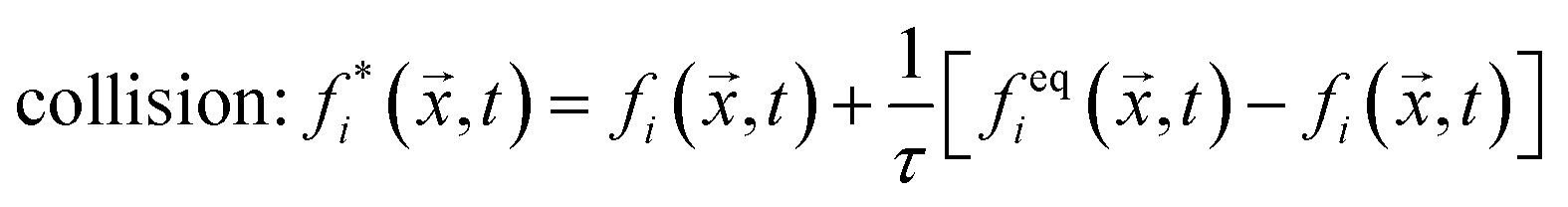 | (1) |
streaming: fi( + ![[c with combining right harpoon above (vector)]](https://www.rsc.org/images/entities/i_char_0063_20d1.gif) iΔt,t + Δt) = fi*(,t), iΔt,t + Δt) = fi*(,t), | (2) |
,t) is the discretized particle distribution function with the index i indicating the velocity vectors, feqi is an expansion of the Maxwell–Boltzmann distribution up to second order in the mean velocity, and τ is a typical relaxation time from the BGK model.
 | ||
| Fig. 2 Set of velocity vectors for the D3Q19 implementation of the LBM. Six vectors point to the center of the faces, 12 to the center of the edges, and one is the zero velocity. | ||
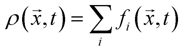
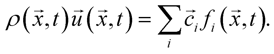
Macroscopic quantities like the density ρ or the momentum density ρ![[u with combining right harpoon above (vector)]](https://www.rsc.org/images/entities/i_char_0075_20d1.gif) correspond to the first two moments of the distribution function with respect to velocity:
correspond to the first two moments of the distribution function with respect to velocity:
 | (3) |
 | (4) |
 | (5) |
 is the speed of sound measured in LBM units. It is important to note that the LBM is only valid for small Mach numbers Ma = umax/cs to ensure the incompressibility of the Newtonian fluid. We chose the maximum flow velocity such that Ma ≤ 0.1 for all our simulations, which corresponds to density variations of less than 1%.
Simulations with immersed-boundaries like our deformable capsules show the best accuracy for relaxation times τ ≤ 1 or viscosities ν ≤ 1/6, according to eqn (5) with LBM time step δt = 1. Due to this restriction we tuned the Reynolds number by adjusting the Mach number while keeping the viscosity fixed ν = 1/6. This is only possible up to a Reynolds number Re ≈ 50, depending on the number of lattice cells. For higher Re we fixed Ma = 0.1 and reduced the viscosity ν.
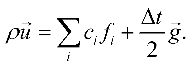
To simulate the pressure-driven Poiseuille flow, we implemented a constant body force ![[g with combining right harpoon above (vector)]](https://www.rsc.org/images/entities/i_char_0067_20d1.gif) following the Guo force scheme.50 In this scheme the fluid momentum density at each time step is modified according to
following the Guo force scheme.50 In this scheme the fluid momentum density at each time step is modified according to
 | (6) |
Our simulations were conducted with a length-to-width ratio of L/2w = 4 using periodic boundary conditions along the channel (z-axis). As resolution for the lattice-Boltzmann solver, we chose 120 cubic unit cells along the full width of the channel, when we recorded trajectories of the capsules, and 90 cells for determining the lift-force profiles. Especially for soft particles (La = 1 to 10) and high Reynolds numbers (Re = 100) the lift force was not constant but oscillating in time. To avoid these oscillations, the resolution was enhanced to 180 cells.
2.3 Modeling a deformable capsule
To couple the deformable capsule to the fluid, we use the immersed-boundary method.52–54 In this method the capsule is modeled with a deformable Lagrangian grid, which moves in the fixed Eulerian grid of the LBM. The Lagrangian mesh of the undeformed spherical capsule is obtained by starting from an icosahedron and then repeatedly subdividing each triangle into four triangles such that the distance between two neighboring vertices is approximately equal to the lattice spacing of the Eulerian grid. The resolution for the different simulated meshes is given in Table 1. The membrane forces are calculated on the Lagrangian mesh and interpolated to the grid of the fluid. Likewise, the velocities of the mesh vertices are determined by an interpolation from the fluid velocity vectors of the surrounding grid nodes. For both interpolations a weighting function ϕ(r) is used, which averages over all lattice nodes within a distance Δx from the center, where Δx is 2. For further details we refer to ref. 54.| Particle radius a/w | Number of lattice nodes | Number of vertices |
|---|---|---|
| 0.1 | 90 | 1280 |
| 0.1 | 120 | 1280 |
| 0.16 | 90 | 5120 |
| 0.2 | 90 | 5120 |
| 0.2 | 120 | 5120 |
| 0.2 | 180 | 20![[thin space (1/6-em)]](https://www.rsc.org/images/entities/char_2009.gif) 480 480 |
| 0.3 | 90 | 20480 |
| 0.3 | 120 | 20480 |
| 0.4 | 90 | 20480 |
To model the capsule, three contributions need to be considered: in-plane elasticity of the capsule membrane, its bending stiffness, and volume conservation due to the incompressible fluid interior. Elastic deformations are described by the Skalak model, which originally was introduced for red blood cells.55 The elastic energy is written in the strain invariants I1 and I2 of the Green strain tensor as defined in Appendix A.2,
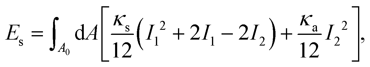 | (7) |
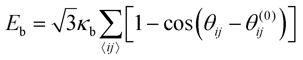
Bending stiffness is needed to prevent buckling of the capsules and the formation of cusps. To quantify bending elasticity, we take the Helfrich functional, which can be discretized on the triangular surface mesh,56,57
 | (8) |
 | (9) |
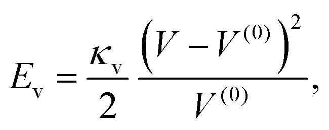
000ρν2/L2 such that the volume changes were less than 1%. To reduce the number of variable parameters, we followed Krüger et al.37 and fixed the ratios of the area and the bending moduli with the shear modulus,| κa/κs = 2 κb/(κsa2) = 2.87 × 10⁻³. | (10) |
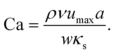
The capillary number Ca, as the ratio between applied viscous shear stress ρνumax/w and typical elastic stress κs/a, describes the deformability of an elastic capsule,
 | (11) |
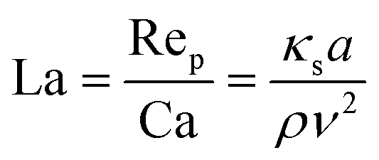 | (12) |
2.4 Measurement of the lift-force profile
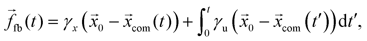
To determine the inertial lift force acting on the capsule, we fix its lateral position and measure the force of the LB fluid on the membrane following ref. 41. To hold the capsule in place, we apply an adjustable force ffb evenly distributed over all the membrane vertices, which compensates the lift force. To calculate this feedback force, we use a proportional-integral (PI) feedback controller.60 The idea is to steer a system parameter, here the lateral position, by an external force ffb in a targeted state. In our case the dynamics of the lateral position of the capsule's center of mass,com, is determined by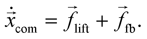 | (13) |
 | (14) |
0 is the targeted lateral position. We choose γx = 1 and γu = 100 in LB units. In steady state, 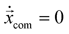 , one obtains lift = −fb. The lift force is averaged over at least 200000 time steps, where the first 20000 time steps, until the system equilibrates, are neglected.
3 Results
3.1 Equilibrium position
We first study in detail the equilibrium position of one single capsule varying particle radius a, its deformability measured by the capillary number Ca or the Laplace number La, and the channel Reynolds number Re. We vary the Laplace number in the interval between 1 (very soft) and 1000 (almost rigid) or the capillary number between 10−4 and 10. For the Reynolds number we choose the values 5, 10, 50, 100.We used two different methods to determine the equilibrium position of the capsule. The first method is closer to the experiment. The particle is put at a specific position and can then move freely. Fig. 3 shows a collection of example trajectories. Especially the small particles with a/w = 0.1 at Re = 10 migrate slowly and do not reach their equilibrium positions on either the diagonal or the x axis, even in the longest simulation runs. The reason is that the lift force driving the particle motion strongly scales with particle radius a and Reynolds number, as discussed in Section 3.3 but also depends on the deformability of the capsule. However, in most cases one clearly sees where the particles migrate to.
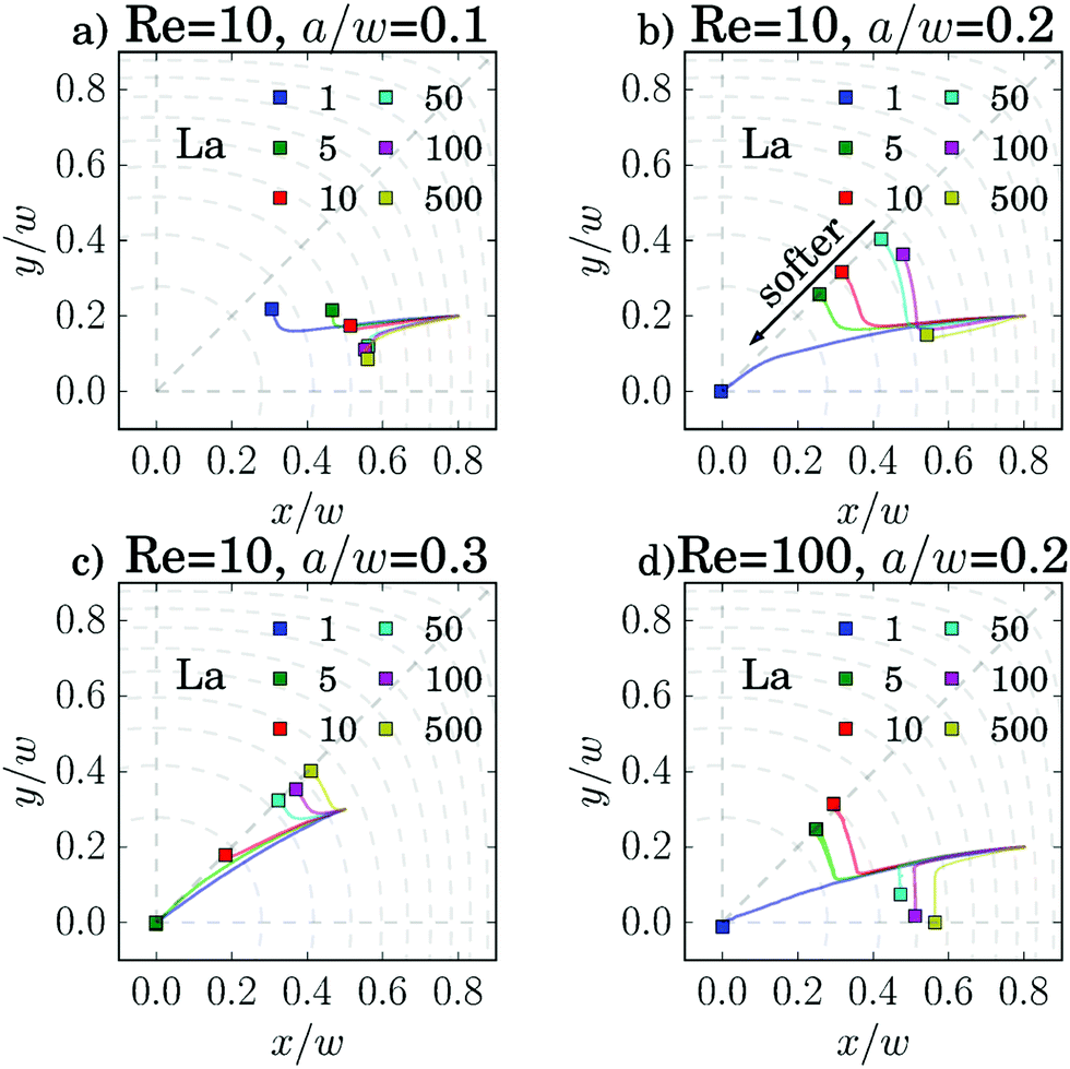 | ||
| Fig. 3 Trajectories of the capsules in the cross-sectional plane of the channel with different rigidities quantified by the Laplace number La. The trajectories are plotted for different particle sizes a/w and Reynolds numbers Re as indicated in (a)–(d). The capsules start at the same position and the endpoint of the trajectories are shown by filled squares. Not all of them reach their equilibrium position on the diagonal or the main axis during the simulations. | ||
As most particles in our study migrate towards the diagonal, we will focus our attention on this axis in the following analysis. Migration towards the main axes and the diagonals has been more thoroughly studied for rigid particles in ref. 27. Roughly speaking, larger particles migrate towards the diagonal, where they are further away from the walls, while smaller particles migrate towards the main axes.
For the particle trajectories, which we visualize in Fig. 3(c), we plot in Fig. 4 the lateral velocity v⊥ in the cross-sectional plane of the channel versus the distance d from the center. All particles start at the same position at a distance d/w = 0.583. The velocity rapidly increases and then gradually decreases to zero as the particles move inwards towards their equilibrium position. Clearly, softer particles (small La) show a larger lateral migration velocity than rigid particles. For the smaller particles in Fig. 3(b) the migration process itself splits into two phases. First, the particles quickly move inwards along the radial direction. This corresponds to the gradual decrease of the lateral velocity as discussed in Fig. 4. When the capsules are close to their final equilibrium distance, the radial movement stops and the lateral velocity is close to zero. Thus, the particles only very slowly drift along the polar direction towards their equilibrium positions. A similar kind of motion was already observed for rigid particles.24
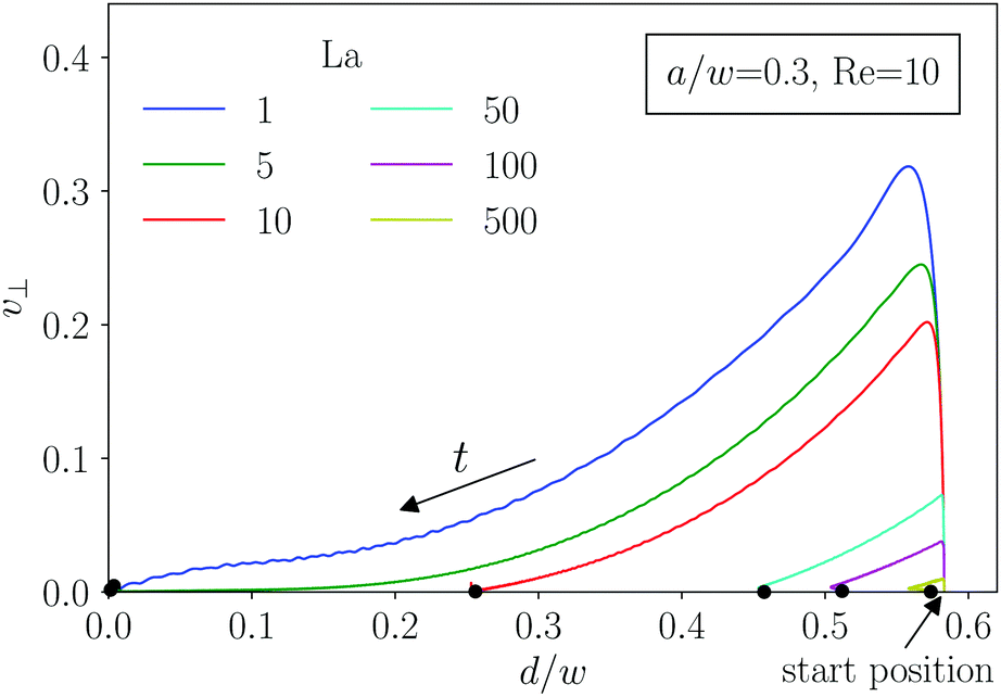 | ||
| Fig. 4 Lateral velocity v⊥ plotted versus the distance d to the channel center for different Laplace numbers La. All particles start at the same initial position (d/w = 0.583) and with time move inwards to their equilibrium positions indicated by a black dot. | ||
To have a computationally more efficient method for determining the equilibrium positions, we also measured lift-force profiles using the method outlined in Section 2.4. The equilibrium positions correspond to the stable fix points. We will discuss the lift-force profiles in more detail in Section 3.3. Both methods agree well, as we demonstrate in Fig. 13 in Appendix A.1. For the following discussion based on Fig. 5 we will take the equilibrium positions determined from the lift-force profiles. The free migration of the capsules indicate that they mostly lie on the diagonals. Only small capsules (a/w = 0.1) and capsules at Re = 100, which are sufficiently rigid (La > 50), clearly migrate towards the x axis. The results on the rigid particles are in agreement with our earlier work.27
 | ||
| Fig. 5 Equilibrium distance deq/w from the channel center: (a) plotted versus Laplace number La for a/w = 0.2 and different Re, inset: deq/w versus capillary number Ca; (b) deq/w plotted versus La for Re = 10 and different a/w, inset: deq/w versus La/(a/w)4. | ||
We now discuss the equilibrium distance from the channel center, deq, in more detail. In the inset of Fig. 5(a) we plot it versus the deformability of the capsule, the capillary number Ca, for different Reynolds numbers Re. All curves show how deformable capsules (large Ca) migrate to the channel center. Making them more rigid by decreasing Ca, the inertial lift force becomes more dominant and drives the capsules away from the center towards the equilibrium distance of solid spheres. Clearly, since the strength of the inertial forces increases with Re, the migration towards the channel walls already starts when the capsules are more deformable (large Ca).
All curves in the inset roughly have the same shape and shift to the right with increasing Re. The capillary number Ca is proportional to the absolute flow velocity umax. Indeed, removing this dependence and plotting the equilibrium distance versus the Laplace number La, which measures the rigidity of the capsule, all curves roughly fall onto one master curve [see main plot of Fig. 5(a)]. This was already observed by Kilimnik et al.35 Deviations from the master curve occur for very rigid capsules (large La), which move closer to the channel walls with increasing Re.22,25,61 Also, the value of La, where the capsule starts to move away from the channel center, is sensitive to Re. This might be due to the fact that the shapes of two capsules, located either in the channel center or close-by, differ strongly as we will discuss below.
Also the particle radius a/w plays an important role for the equilibrium distance, as Fig. 5(b) demonstrates. Larger particles leave the channel center at larger La and thereby assemble closer to the channel center compared to smaller particles. One obvious reason for this behavior is that La ∝ a. However, in addition the lift force, which drives the capsule away from the center, roughly scales with a3 as discussed in ref. 62 and Section 3.3. So, if we plot deqversus La/(a/w)4, the equilibrium distances collapse on a single master curve in the regime where the capsules are deformable [see inset of Fig. 5(b)]. For rigid particles (large La) the curves do not collapse since smaller particles move closer to the channel walls.25,34
3.2 Deformation of the capsules
In Fig. 6 we illustrate the shapes of capsules at their equilibrium positions for different Laplace (La) and Reynolds (Re) numbers. At La = 1 both capsules are located in the channel center and show the expected form of a parachute, which is more visible at larger Reynolds numbers.63 At La = 2.5, the capsules have left the center with deq/w ≈ 0.28 and the deformation is more asymmetric. The capsules become less deformed with increasing La, although the capsules move further away from the channel center, where the viscous shear stresses increase. Interestingly, although the shapes of capsules with the same La differ for the two Re values, in Fig. 5(a) we demonstrated that their equilibrium distances to the channel center are roughly the same independent of Re.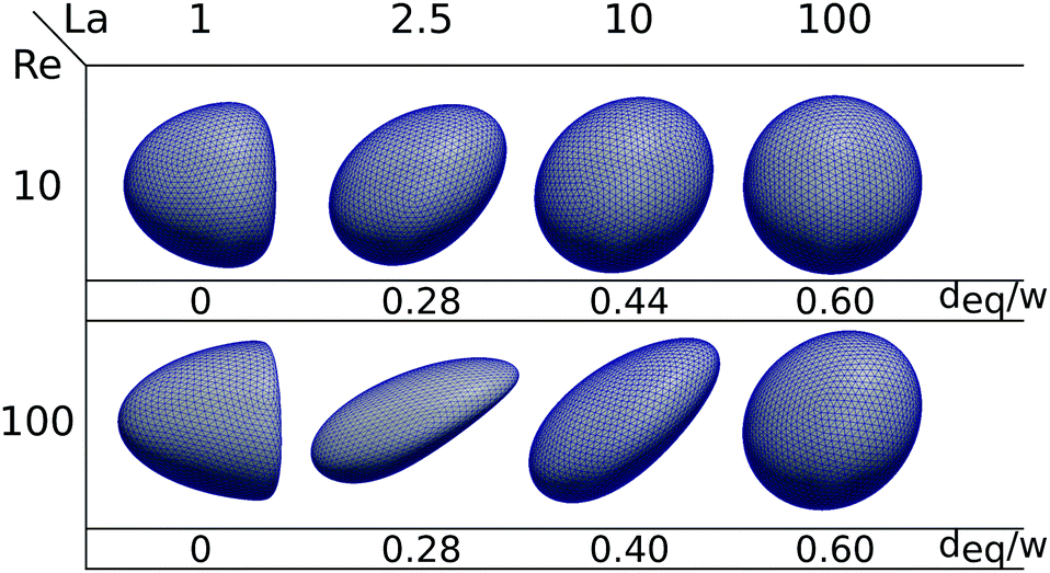 | ||
| Fig. 6 Shapes of the capsules for different Laplace and Reynolds numbers. Below each picture is the corresponding equilibrium distance. | ||
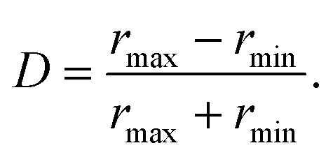
To quantify the deformation of the capsule, we follow64,65 and determine its moment-of-inertia tensor and then the equivalent ellipsoidal particle with the same principal moments of inertia. Now, the smallest and largest semi-axes of the ellipsoid, rmin and rmax, are then used to define the Taylor deformation index,
 | (15) |
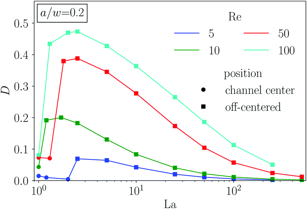 | ||
| Fig. 7 Taylor deformation index D of an elastic capsule at the equilibrium location plotted versus Laplace number La for different Reynolds numbers Re. The symbols correspond to the symmetric shapes in the channel center (•) and to the asymmetric shapes occurring not in the center (■). | ||
3.3 Lift-force profile
The dynamics and equilibrium positions of an elastic capsule are determined by the lift-force profile. In this section we study how the inertial lift force scales with Reynolds and Laplace number as well as particle radius and compare it to rigid particles. For rigid particles with radii much smaller than the channel width the analytical solution22,45 for the lift force predicts the scaling flift ∝ Re2(a/w)4. For larger rigid particles, of similar size as ours, numerical solutions of the Navier–Stokes equations give a scaling proportional to Re2(a/w)3 near the channel center and Re2(a/w)6 near the channel walls.18 To measure the lift force we use the procedure described in Section 2.4. As almost all capsules travel to equilibrium positions on the diagonal, we study the lift-force profiles along this direction.We usually observe the typical form of the lift-force profile with two equilibrium positions of the capsule, where the lift force vanishes [see, for example, Fig. 8(a)]: the unstable fix point in the channel center (d = 0) and one stable fix point between channel center and walls. In the previous section we found that the equilibrium position is almost independent of the Reynolds number, in particular, in an intermediate range of capsule rigidity measured by La. When we measure the lift-force profile for different Reynolds numbers while keeping the particle radius and the Laplace number fixed, this is also visible in the lift-force profiles as all zero crossings coincide [see Fig. 8(a)]. Furthermore, the profiles for small Re fall on top of each other when we scale flift by Re2. This scaling is confirmed in Fig. 3(b), where we plot the maximum lift force versus Re. Only for high Reynolds number (Re = 100) we obtain a deviation from flift ∝ Re2. Indeed, by measuring the particle–wall interaction of rigid particles, the authors of ref. 46 noticed an increase of the wall lift coefficient around Re ≈ 100 due to an imperfect bifurcation of the wake structure. This might explain our observation. However, in total the scaling law flift ∝ Re2 also seems to be valid for soft spheres at moderate Re.
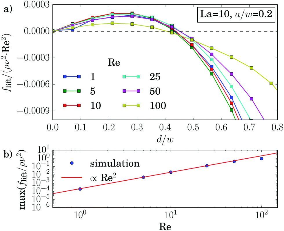 | ||
| Fig. 8 (a) Inertial lift force flift along the diagonal in units of ρν2Re2 plotted versus distance d/w to the center for different Reynolds numbers. Other parameters are La = 10 and a/w = 0.2. (b) Maximum of flift plotted versus Re. | ||
Fig. 9(a) confirms the scaling flift ∝ (a/w)3 for small distances, while closer to the walls the force profiles clearly differ. Strong deviations also occur for larger particles with a/w ≥ 0.3, which is also visible in the maximum lift force plotted versus a/w in Fig. 9(b). This is in contrast to ref. 25 and 62, where the scaling was verified for rigid particles with radii up to a/w = 0.38. The different behavior can be attributed to the deformability of the capsules. Indeed, for La = 500 we verify the scaling up to a particle radius of a/w = 0.4 as demonstrated by Fig. 14 in Appendix A.3.
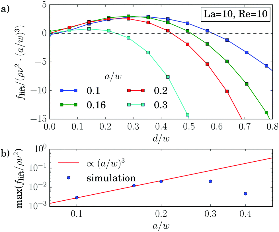 | ||
| Fig. 9 (a) Inertial lift force flift along the diagonal in units of ρν2(a/w)3 plotted versus distance d/w to the center for different particle radii a/w. Other parameters are La = 10 and Re = 10. (b) Maximum of flift plotted versus a/w. | ||
For increasing Laplace number the lift-force profiles approach the limit of a rigid capsule [see Fig. 10(a)]. Making the particles softer, the stable equilibrium position moves towards the channel center and ultimately for La = 1 reaches the center, as already discussed in Section 3.1. Also, the maximum value of the lift force decreases the softer the particles become as illustrated in Fig. 10(b).
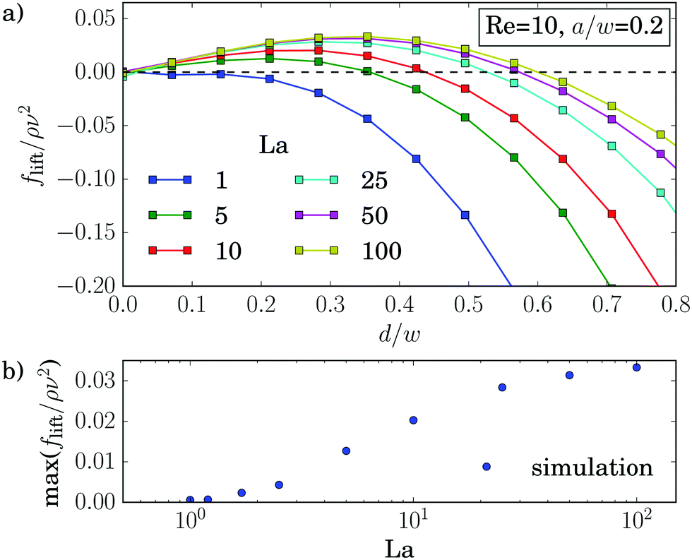 | ||
| Fig. 10 (a) Inertial lift force flift along the diagonal in units of ρν2 plotted versus distance d/w to the center for different Laplace numbers. Other parameters are Re = 10 and a/w = 0.2. (b) Maximum of flift plotted versus La. | ||
3.4 External control force
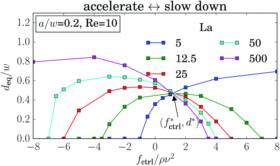
Experiments39 and simulations27 showed that the lateral position of rigid particles can be controlled by an external force, applied along the channel axis. Depending on its direction it either speeds up or slows down the particle relative to the channel flow. This changes the relative velocity between particle surface and surrounding fluid. Thereby, the dynamic pressure varies along the surface, which causes the lateral motion of the particle known as Saffman effect.40 In our simulations we apply a constant force on the elastic capsule evenly distributed on the membrane vertices along the axial direction. We observe that the shape of the capsules is hardly influenced by the external control force. It is mainly determined by the local shear gradient, which depends on the distance from the channel center.In the following discussion we choose the convention that a positive force is directed against the flow and thus slows down the particle. In Fig. 10 we plot the equilibrium distance to the channel center as a function of the external control force fctrl. As before, we determined the equilibrium positions from the stable fix points of the lift-force profiles. For rigid capsules (La = 500) the results agree with previous simulations:27 when these particles are slowed down (fctrl > 0), they move towards the channel center and ultimately reach it for sufficiently large fctrl > 0, while accelerated particles move closer to the channel walls. However, for strongly negative control forces a decrease in the equilibrium distance is observable. This behavior is clearer visible for La = 50. We observe the softer the capsules are, the more does the maximum equilibrium distance move to larger and even positive control forces. Furthermore, the maximum equilibrium distance decreases until at around La ≈ 12.5, where the curve is symmetric about its maximum. For even softer capsules it increases again. As a consequence, soft particles (La = 5) behave opposite to rigid particles: when slowed down, they move away from the channel center, while when moving faster (fctrl < 0), they approach the center and ultimately stay there.
Förtsch et al.66 observed a similar kind of migration for soft capsules under gravity in pure Stokes flow. They showed by simulation and analytical calculations that this can be explained by the anisotropic drag coefficient. Due to their elongated shape (see Fig. 6) the resistance of the soft capsules is different along their main axes. By pulling on such a deformed capsule, it migrates in the direction of the smallest drag coefficient, which is along their longest axis.
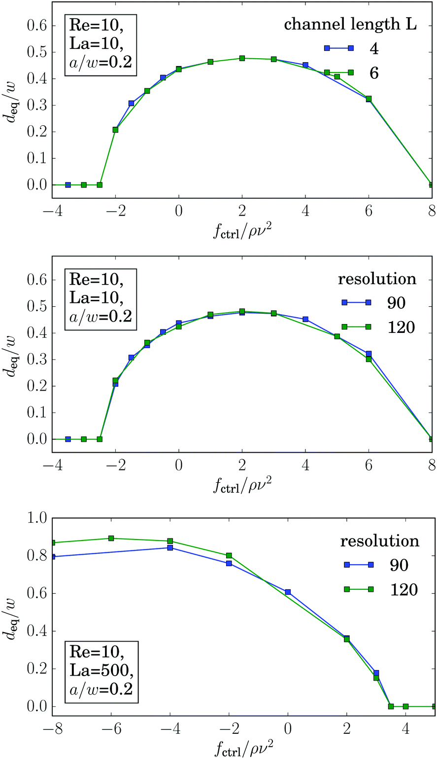
Even more interesting, we find that all curves for different La intersect in one point at a positive control force of about fctrl* = 1.2ρν2. At this control force all particles assemble at the same equilibrium distance deq* independent of their deformability. This property seems to be generic. We also find it for other Reynolds numbers as illustrated in Fig. 15 of Appendix A.4. While the intersection point moves to higher control forces with increasing Reynolds number, in fact, fctrl* ∝ Re as Fig. 12 demonstrates, the distance from the channel center stays almost the same at ![[d with combining tilde]](https://www.rsc.org/images/entities/i_char_0064_0303.gif) /w ≈ 0.46. We do not have a clear understanding of this behavior. However, we checked that it is generic and not a numerical artifact. In particular, this behavior does not change when we increase the channel length to investigate the influence of the periodic boundary condition or when we increase the resolution of the lattice-Boltzmann grid to check for discretization errors (see Fig. 15 in Appendix A.4).
/w ≈ 0.46. We do not have a clear understanding of this behavior. However, we checked that it is generic and not a numerical artifact. In particular, this behavior does not change when we increase the channel length to investigate the influence of the periodic boundary condition or when we increase the resolution of the lattice-Boltzmann grid to check for discretization errors (see Fig. 15 in Appendix A.4).
Using such an external force, allows a much finer control of the particle's equilibrium position. For example, in the absence of a control force (fctrl = 0 in Fig. 11) the equilibrium position of particles with La = 5 and La = 12.5 are quite close to each other. By applying fctrl = −1ρν2 the softer particle moves towards the center while the equilibrium position of the less deformable particle hardly changes. This effect should help to enhance particle separation based on its deformability. One way to implement an external force experimentally could be using buoyancy where fluid and particles have a different density.
 | ||
| Fig. 11 Equilibrium distance deq plotted versus the external control force fctrl for different Laplace numbers La. Other parameters are Re = 10 and a/w = 0.2. | ||
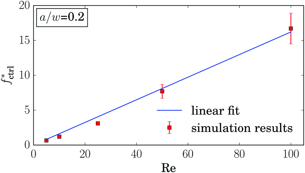 | ||
| Fig. 12 Control force of the intersection point fctrl* plotted versus Reynolds number Re. At lower Reynolds numbers the errorbars are on the order of the symbol size. | ||
4 Conclusions
Manipulating deformable capsules by hydrodynamic flow in the regime of intermediate Reynolds numbers has a large variety of applications, e.g., for cell sorting or probing. The high fluid velocities allow a high throughput and the resulting inertial focusing can be used to separate and steer particles towards desired positions within a channel. In this work we studied the equilibrium positions of soft capsules while immersed in a Poiseuille flow through a quadratic channel. We find that most particles assemble along the diagonal of the channel. The softer the particles are the closer they move towards the channel center. Their final equilibrium distance depends on the particle deformability, its radius and the channel Reynolds number. By introducing the Laplace number as ratio of elastic force to the intrinsic viscous force scale, the equilibrium position for different Reynolds numbers collapse on a single master curve. The equilibrium distance is thus independent of the flow velocity. Additionally, we also identify such a date collapse for different particle radii.In contrast to the equilibrium distance we find that the deformation of the capsules strongly depends on the Reynolds number. The deformation of the off-centered capsules increases with decreasing Laplace number although the capsules migrate in areas with a smaller shear gradient. Very soft capsules assemble at the channel center and have a symmetric parachute shape.
The lift-force profiles of deformable capsules behave pretty much the same as those of rigid particles, where the lift force scales as flift ∝ Re2(a/w)3. For deformable capsules, we find deviations from this scaling law only for high Reynolds number (Re = 100) and large particles (a/w = 0.3). We were not able to identify a similar scaling involving the Laplace number. For decreasing La, the stable equilibrium position moves towards the channel center and the maximum value of the lift force decreases until only a stable fixpoint in the channel center remains.
Finally, we demonstrated that the particle equilibrium position can be controlled by an external force along the channel axis. For almost rigid particles (La = 500) we confirmed previous results,27 but found a new behavior for soft particles. While rigid particles migrate towards the channel center when they are slowed down, moderately soft particles with La ≈ 12.5 migrate towards the channel center both for positive and negative control forces. For even lower La the capsules behave opposite to rigid particles as they move towards the channel wall when slowed down. Interestingly, we observe that all graphs with different Laplace numbers intersect in one point at a non-zero control force.
Cancer cells are softer than healthy cells.2 Using an external control force, enhances the sensitivity to separate them based on the lateral locations they assume in microchannels. Thus, our new theoretical insights might prove useful in developing new biomedical devices to probe and separate cells based on their size and deformability.
A Appendices
A.1 Determining the equilibrium distance
To determine the equilibrium distance of the elastic capsule from the channel center, we considered two different methods as described in Section 3.1 (Fig. 13).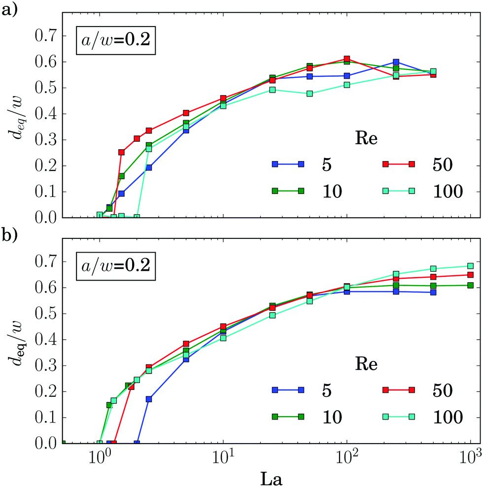 | ||
| Fig. 13 Equilibrium distance from the center as a function of the Laplace number determined by two different methods. (a) Particles are placed in the flow and migrate freely to their equilibrium position; (b) the equilibrium distance is extracted from the stable fix points of the lift-force profiles. Both plots agree quite well. | ||
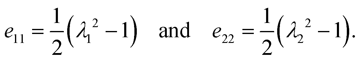
A.2 Green strain tensor
Skalak et al.55 introduced a model for the strain energy of the membrane of a red blood cell. It is formulated in the framework of finite strain theory, which investigates the deformation of a body relative to a reference configuration. We denote the reference coordinates by and the coordinates of the deformed state by ![[y with combining right harpoon above (vector)]](https://www.rsc.org/images/entities/i_char_0079_20d1.gif) . In the coordinate system, where the local Jacobi matrix ∂yi/∂xj is diagonal, the extension ratios λ1 and λ2 are given by
. In the coordinate system, where the local Jacobi matrix ∂yi/∂xj is diagonal, the extension ratios λ1 and λ2 are given by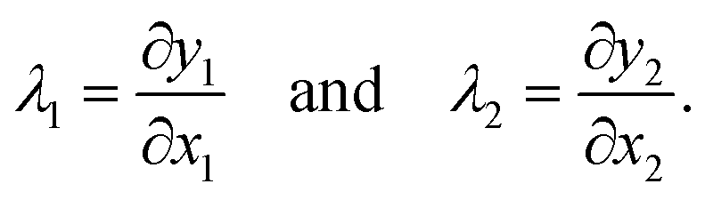 | (A1) |
 | (A2) |
 | (A3) |
. The Piola–Kirchoff stress tensor is related to the Cauchy stress tensor by | (A4) |
| I1 = 2(e11 + e22) = λ12 + λ22 − 2 | (A5) |
| I2 = 4e11e22 + I1 = λ12λ22 − 1. | (A6) |
A.3 Lift force profile for stiffer particles
For soft particles we obtain a deviation from the scaling with the particle radius, flift ∝ (a/w)3, already at small radii (Fig. 9). As its origin we suspect the deformability of the capsules. Indeed, by increasing the particle stiffness, we obtain an agreement with the scaling law up to a particle radius of a/w = 0.4 (Fig. 14).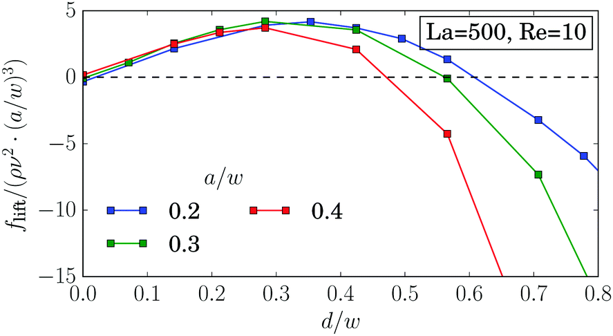 | ||
| Fig. 14 Inertial lift force flift along the diagonal in units of ρν2(a/w)3 for different particle radii for almost rigid particles. | ||
A.4 Equilibrium distance for external control force
Fig. 15 shows the equilibrium distance plotted versus the control force for different Laplace numbers and Reynolds numbers. The curves for different La intersect in one point. This is valid for all Reynolds numbers. With increasing Re the intersection point moves towards higher forces while the equilibrium distance only varies little.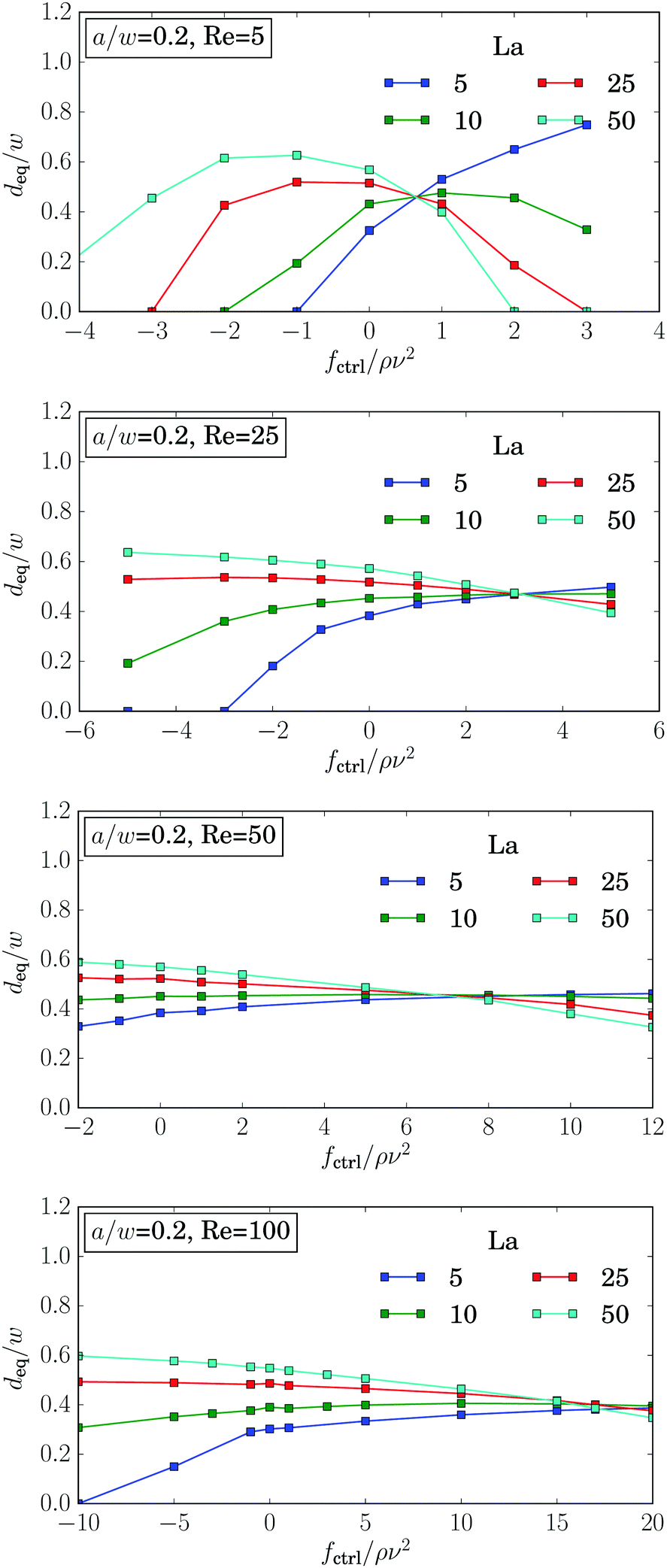 | ||
| Fig. 15 The equilibrium distance deq plotted versus control force fctrl for different Laplace numbers La and Reynolds numbers Re = 5, 25, 50, 100 for particle radius a = 0.2w. | ||
As demonstrated in Fig. 16, the graphs for the equilibrium distance plotted versus control force is independent of the channel length L, the resolution of the lattice-Boltzmann grid. Only for rigid particles (La = 500), one observes small deviations, when the particles are located close to the walls.
 | ||
| Fig. 16 The equilibrium distance deq plotted versus control force for different channel lengths (top) and different resolutions of the lattice-Boltzmann grid for La = 10 (middle) and La = 500 (bottom). | ||
Acknowledgements
We thank C. Prohm for providing the source code and for initial work in the project. We acknowledge support from the Deutsche Forschungsgemeinschaft in the framework of the Collaborative Research Center SFB 910.References
- G. Y. H. Lee and C. T. Lim, Trends Biotechnol., 2007, 25, 111–118 CrossRef CAS PubMed.
- S. Suresh, Acta Biomater., 2007, 3, 413–438 CrossRef PubMed.
- J. Guck, S. Schinkinger, B. Lincoln, F. Wottawah, S. Ebert, M. Romeyke, D. Lenz, H. M. Erickson, R. Ananthakrishnan, D. Mitchell, J. Käs, S. Ulvick and C. Bilby, Biophys. J., 2005, 88, 3689–3698 CrossRef CAS PubMed.
- H. A. Cranston, C. W. Boylan, G. L. Carroll, S. P. Sutera, J. R. Williamson, I. Y. Gluzman and D. J. Krogstad, Science, 1984, 223, 400–403 CAS.
- S. Suresh, J. Spatz, J. P. Mills, A. Micoulet, M. Dao, C. T. Lim, M. Beil and T. Seufferlein, Acta Biomater., 2005, 1, 15–30 CrossRef CAS PubMed.
- O. Otto, P. Rosendahl, A. Mietke, S. Golfier, C. Herold, D. Klaue, S. Girardo, S. Pagliara, A. Ekpenyong, A. Jacobi, M. Wobus, N. Töpfner, U. F. Keyser, J. Mansfeld, E. Fischer-Friedrich and J. Guck, Nat. Methods, 2015, 12, 199–202 CrossRef CAS PubMed.
- H. W. Hou, A. A. S. Bhagat, A. G. Lin Chong, P. Mao, K. S. Wei Tan, J. Han and C. T. Lim, Lab Chip, 2010, 10, 2605 RSC.
- L. R. Huang, E. C. Cox, R. H. Austin and J. C. Sturm, Science, 2004, 304, 987–990 CrossRef CAS PubMed.
- T. M. Geislinger, B. Eggart, S. Braunmüller, L. Schmid and T. Franke, Appl. Phys. Lett., 2012, 100, 183701 CrossRef.
- D. Bell, C. Wongsrichanalai and J. W. Barnwell, Nat. Rev. Microbiol., 2006, 4, S7–S20 CrossRef PubMed.
- G. Coupier, B. Kaoui, T. Podgorski and C. Misbah, Phys. Fluids, 2008, 20, 111702 CrossRef.
- F. Risso, F. Collé-Paillot and M. Zagzoule, J. Fluid Mech., 2006, 547, 149–173 CrossRef CAS.
- P. Bagchi, Biophys. J., 2007, 92, 1858–1877 CrossRef CAS PubMed.
- G. R. Lázaro, A. Hernández-Machado and I. Pagonabarraga, Soft Matter, 2014, 10, 7207–7217 RSC.
- C. Bächer, L. Schrack and S. Gekle, Phys. Rev. Fluids, 2017, 2, 013102 CrossRef.
- B. Kaoui, G. H. Ristow, I. Cantat, C. Misbah and W. Zimmermann, Phys. Rev. E: Stat., Nonlinear, Soft Matter Phys., 2008, 77, 021903 CrossRef CAS PubMed.
- G. Segré and A. Silberberg, Nature, 1961, 189, 209–210 CrossRef.
- D. Di Carlo, Lab Chip, 2009, 9, 3038 RSC.
- J. P. Matas, J. F. Morris and E. Guazzelli, Oil Gas Sci. Technol., 2004, 59, 59–70 Search PubMed.
- D. D. Carlo, D. Irimia, R. G. Tompkins and M. Toner, Proc. Natl. Acad. Sci. U. S. A., 2007, 104, 18892–18897 CrossRef PubMed.
- A. A. S. Bhagat, S. S. Kuntaegowdanahalli and I. Papautsky, Microfluid. Nanofluid., 2009, 7, 217–226 CrossRef CAS.
- E. S. Asmolov, J. Fluid Mech., 1999, 381, 63–87 CrossRef CAS.
- J. A. Schonberg and E. J. Hinch, J. Fluid Mech., 1989, 203, 517–524 CrossRef CAS.
- B. Chun and A. J. C. Ladd, Phys. Fluids, 2006, 18, 031704 CrossRef.
- C. Prohm, M. Gierlak and H. Stark, Eur. Phys. J. E: Soft Matter Biol. Phys., 2012, 35, 80 CrossRef CAS PubMed.
- W. Lee, H. Amini, H. A. Stone and D. Di Carlo, Proc. Natl. Acad. Sci. U. S. A., 2010, 107, 22413–22418 CrossRef CAS PubMed.
- C. Prohm and H. Stark, Lab Chip, 2014, 14, 2115 RSC.
- D. Salac and M. J. Miksis, J. Fluid Mech., 2012, 711, 122–146 CrossRef.
- A. J. Mach and D. Di Carlo, Biotechnol. Bioeng., 2010, 107, 302–311 CrossRef CAS PubMed.
- S. K. Doddi and P. Bagchi, Int. J. Multiphase Flow, 2008, 34, 966–986 CrossRef CAS.
- D.-K. Sun and Z. Bo, Int. J. Heat Mass Transfer, 2015, 80, 139–149 CrossRef.
- B. Kim, C. B. Chang, S. G. Park and H. J. Sung, Int. J. Heat Fluid Flow, 2015, 54, 87–96 CrossRef.
- Z. Wang, Y. Sui, A.-V. Salsac, D. Barthès-Biesel and W. Wang, J. Fluid Mech., 2016, 806, 603–626 CrossRef.
- S. C. Hur, N. K. Henderson-MacLennan, E. R. B. McCabe and D. Di Carlo, Lab Chip, 2011, 11, 912 RSC.
- A. Kilimnik, W. Mao and A. Alexeev, Phys. Fluids, 2011, 23, 123302 CrossRef.
- Y.-L. Chen, RSC Adv., 2014, 4, 17908–17916 RSC.
- T. Krüger, B. Kaoui and J. Harting, J. Fluid Mech., 2014, 751, 725–745 CrossRef.
- S. J. Shin and H. J. Sung, Phys. Rev. E: Stat., Nonlinear, Soft Matter Phys., 2011, 83, 046321 CrossRef PubMed.
- Y. W. Kim and J. Y. Yoo, Lab Chip, 2009, 9, 1043 RSC.
- P. G. T. Saffman, J. Fluid Mech., 1965, 22, 385–400 CrossRef.
- C. Prohm, N. Zöller and H. Stark, Eur. Phys. J. E: Soft Matter Biol. Phys., 2014, 37, 36 CrossRef PubMed.
- C. Prohm, F. Tröltzsch and H. Stark, Eur. Phys. J. E: Soft Matter Biol. Phys., 2013, 36, 118 CrossRef PubMed.
- H. Bruus, Theoretical Microfluidics, Oxford University Press, Oxford, New York, 2008 Search PubMed.
- R. Fåhraeus, Physiol. Rev., 1929, 9, 241–274 Search PubMed.
- G. Segré and A. Silberberg, J. Fluid Mech., 1962, 14, 136–157 CrossRef.
- L. Zeng, S. Balachandar and P. Fischer, J. Fluid Mech., 2005, 536, 1–25 CrossRef.
- S. Succi, The Lattice Boltzmann Equation for Fluid Dynamics and Beyond, Clarendon Press, Oxford University Press, Oxford, New York, 2001 Search PubMed.
- P. L. Bhatnagar, E. P. Gross and M. Krook, Phys. Rev., 1954, 94, 511–525 CrossRef CAS.
- B. Dünweg and A. J. Ladd, Advances in Polymer Science, Springer Berlin Heidelberg, 2008, pp. 1–78 Search PubMed.
- Z. Guo, C. Zheng and B. Shi, Phys. Rev. E: Stat., Nonlinear, Soft Matter Phys., 2002, 65, 046308 CrossRef PubMed.
- The Palabos Project, 2013, http://www.palabos.org/.
- C. S. Peskin, PhD thesis, Albert Eistein College of Medicine, 1972.
- C. S. Peskin, Acta Numer., 2002, 11, 479–517 CrossRef.
- T. Krüger, F. Varnik and D. Raabe, Comput. Math. Appl., 2011, 61, 3485–3505 CrossRef.
- R. Skalak, A. Tozeren, R. P. Zarda and S. Chien, Biophys. J., 1973, 13, 245 CrossRef CAS PubMed.
- W. Helfrich, Z. Naturforsch., C: J. Biosci., 1973, 28, 693–703 CAS.
- G. Gompper and D. M. Kroll, J. Phys., 1996, 6, 1305–1320 Search PubMed.
- Soft Matter, ed. G. Gompper and M. Schick, Wiley-VCH, Weinheim, 2006 Search PubMed.
- T. Krüger, D. Holmes and P. V. Coveney, Biomicrofluidics, 2014, 8, 054114 CrossRef PubMed.
- K. J. Åström and R. M. Murray, Feedback Systems: An Introduction for Scientists and Engineers, Princeton University Press, Princeton, 2008 Search PubMed.
- J.-P. Matas, J. F. Morris and É. Guazzelli, J. Fluid Mech., 2004, 515, 171–195 CrossRef.
- D. Di Carlo, J. F. Edd, K. J. Humphry, H. A. Stone and M. Toner, Phys. Rev. Lett., 2009, 102, 094503 CrossRef PubMed.
- J. Horwitz, P. Kumar and S. Vanka, Int. J. Multiphase Flow, 2014, 67, 10–24 CrossRef CAS.
- G. I. Taylor, Proc. R. Soc. London, Ser. A, 1934, 146, 501–523 CrossRef CAS.
- S. Ramanujan and C. Pozrikidis, J. Fluid Mech., 1998, 361, 117–143 CrossRef CAS.
- A. Förtsch, M. Laumann, D. Kienle and W. Zimmermann, 2017, arXiv:1704.06590 [cond-mat.soft].
| This journal is © The Royal Society of Chemistry 2017 |