
 Open Access Article
 This Open Access Article is licensed under a
 Creative Commons Attribution 3.0 Unported Licence
Interfacial interaction and enhanced image contrasts in higher mode and bimodal mode atomic force microscopy
Shuai Shi ,
Dan Guo* and
Jianbin Luo*
,
Dan Guo* and
Jianbin Luo*
State Key Laboratory of Tribology, Tsinghua University, Beijing 100084, China. E-mail: guodan26@tsinghua.edu.cn; luojb@tsinghua.edu.cn
First published on 5th December 2017
Abstract
Higher mode and bimodal atomic force microscopy (AFM) are two recently developed imaging modes of dynamic AFM for improving resolution. In higher mode, the higher flexural mode of the cantilever instead of the traditional fundamental eigenmode is excited. In bimodal mode, two flexural modes of the cantilever are simultaneously excited for obtaining more information about the properties of the material. The first three flexural modes for higher mode and superposition of two excitation signals for bimodal mode are explored and compared by imaging a polymer blend of polystyrene (PS) and low density polyethylene (LDPE). The effects of different operating conditions of the two imaging modes are researched to improve image contrast and material discrimination. Dissipated power and virial are employed to explain the origin of contrast for the complex and highly nonlinear dynamical tip-sample interfacial system. Amplitude and phase contrasts of each single mode and bimodal mode are calculated by Ashman's D statistical equation. It is found that higher single modes with small free amplitudes show enhanced phase contrast. The bimodal of the first and the third modes gains a clear advantage over the bimodal of the first and second modes for phase and amplitude image contrasts. In addition, the best contrast of bimodal imaging occurs when it is a combination of a large free amplitude for the first mode and a small free amplitude for the third mode.
1. Introduction
Amplitude modulated atomic force microscopy (AM-AFM)1,2 has been widely applied to a variety of materials for nanoscale imaging and mechanical characterization. In recent years, higher modes3–6 and multiple frequency AFM7–10 have been new extensions of the conventional amplitude modulated mode for high resolution imaging of compositional materials. In higher modes, the cantilever is excited by using one of the higher flexural modes instead of the first eigenmode. While in multiple frequency techniques, the cantilever is driven at multiple resonant frequencies. Typically, the multiple frequency mode provides extra response channels of amplitude and phase which can be used to characterize hidden features. Bimodal mode,11–14 most common one of multiple frequency AFM, has been first proved the ability of mapping compositional materials in enhanced resolution and sensitivity by Rodriguez and Garcia. Two lock-in amplifiers are employed to demodulate signals with respect to both driving frequencies in bimodal mode. Amplitude of the first mode is kept constant by feedback control system and height provides the topography information of sample. The second excitation is not constrained to map changes in mechanical, magnetic or electrical properties by recording the variation of amplitude and phase in the second mode.8,15Enhanced phase contrast on a soft biological sample by driving the third eigenmode of a v-shaped silicon cantilever was observed by Stark et al.3 The higher mode amplitude was used as the feedback loop error signal in single mode. Martinez et al.13 demonstrated that bimodal AFM was more sensitive to compositional changes and made compatible high resolution imaging of isolated IgG antibodies under very low forces. Sommerhalter et al.16 have reported on Kelvin probe microscopes using the fundamental eigenmode for topography imaging and the second flexural mode for probing the electrostatic properties. Although previous researches have shown the ability of higher mode and bimodal mode, it is important to understand what pivotal roles of imaging parameters such as free amplitudes and setpoint of each mode play. In most previous bimodal works, free amplitude in first mode is always set to be one order of magnitude higher than that in higher mode. In addition, they prefer to select the first two flexural modes of the cantilever in bimodal experiments. The influence of higher mode except the second one and great amplitudes of higher mode on imaging are lack of research.
In this present work, a standard sample PS-LDPE polymer blend was chosen because of its features of multicomponent and representative. We imaged the polymer blend by higher single modes and bimodal modes. Driving signals of the single mode were the first, second and third flexural modes of the cantilever, respectively. Different free amplitudes and amplitude setpoint ratios were defined in the experiments. Driving signals of bimodal were the combination of the first and second, and first and third modes, respectively. Similarly, different free amplitudes of both driving signals were tried in bimodal imaging mode. For the complex nonlinear interaction system of the tip-sample, dissipated power and virial have been employed to plot the relative dominance of conservative and non-conservation (dissipative) interfacial interactions.17–19 Energy transfer or change between two modes may determine the origin of the contrast.20 Phase contrast is closely connected to the magnitude of the dynamic dissipated power per vibrating cycle during the cantilever scanning on the surface by AM-AFM mode.21 Additionally, virial theorem establishes a connection between phase and the time-averaged interaction force.22 Virial can be interpreted as the average stored energy (potential energy) of the tip-sample interaction.23,24 Average dissipated power Pi and virial Vi for each mode were calculated for PS and LDPE images obtained by the single and bimodal modes, respectively. Expressions of Pi and Vi for each mode are the followings25,26
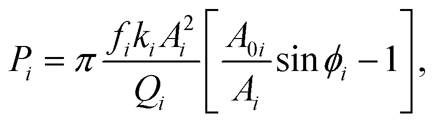 | (1) |
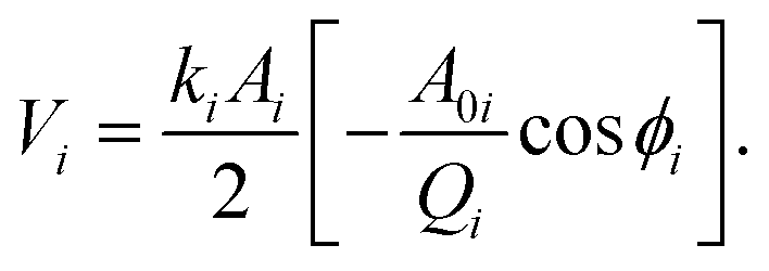 | (2) |
Based on quantitative contrast of amplitude and phase, operating conditions can be optimized. To quantify image contrast at different free amplitudes and variation setpoint ratios, pixel values can be extracted and calculated the histogram of response from each phase image. It may appear as two distinct peaks which is a continuous probability distribution. Fit the normalized histograms and the bimodal distribution function is given by27
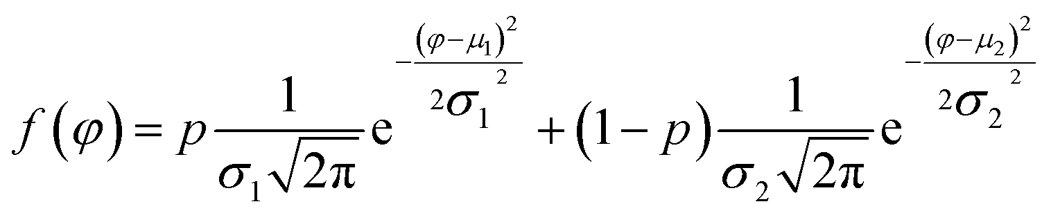 | (3) |
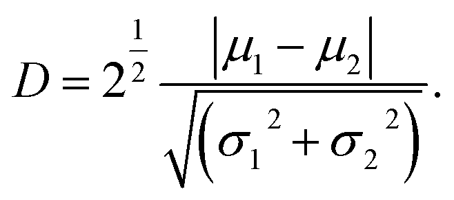 | (4) |
Contrast of a series of single and bimodal experiments on PS-LDPE polymer blend are calculated and summarized. High modes with small free amplitudes show better contrast between two different components. Bimodal AFM also shows excellent contrast by extra response signals, especially for the combination of the first and third modes. Regular changes of contrast which depend on the choice of operation parameters and driving modes will be analyze and discussed here.
2. Experimental details
We performed high frequency single and bimodal imaging experiments using a commercial set of Cypher AFM (Asylum Research, Santa Barbara, CA) equipped with wide bandwidth circuit and high frequency cantilever holders. The polymer blend of polystyrene (PS) (EPS ≈ 2.0 GPa) and low density polyethylene (LDPE) (ELDPE ≈ 0.1 GPa) purchased from Bruker Nano Inc. was used for all designed experiments. Circular domains (LDPE) are mixed in substrate (PS matrix). The inverse optical lever sensitivities (InvOLS) were calibrated from dynamic amplitude approaching curves on a fleshly cleaved mica surface for the first, second and third flexural modes. Based on the equipartition theorem, the spring constants k1, k2, k3 can be obtained via fitting the thermal data around their respective peak which are gathered from thermal noise power spectra method.30 At the same time, three fundamental flexural resonance frequencies and quality factors are calculated. Calibrating a frequently-used cantilever AC240 with this method, the first, second and third flexural resonance frequencies are f1 = 80.510 kHz, f2 = 482.299 kHz, f3 = 1.318 MHz; three dynamic spring constants are k1 = 2.22 N m−1, k2 = 89.46 N m−1 and k3 = 483.7 N m−1. In addition, quality factors of three modes are Q1 = 184.1, Q2 = 475.8 and Q3 = 615.5, respectively.The tip-cantilever system was driven by user-fixed amplitudes close to the free oscillation resonance frequencies. In single experiments, different free amplitudes A0 (20 nm, 30 nm and 40 nm) of the first, second and the third flexural modes were chosen, and the amplitude setpoint ratios are around 0.05–0.85. In the resonance condition, the phase offset between driving force signal and tip deflection is always 90 degrees. In bimodal experiments, different values of the main amplitude A01 (free amplitude of first mode) were also chosen 20 nm, 30 nm and 40 nm. Varying free amplitudes of the second mode (1–50 nm) or the third mode (1–20 nm) were used as another drive signal in bimodal mode. When the tip approaches the surface, tip-sample interaction forces caused changes in both amplitude and phase of the vibrating cantilever. During the whole experiment process, the second free amplitude A02 or A03 decreased gradually. Amplitude change of first mode was used as the feedback signal. If the phase shift was positive, the imaging mode was generally considered as attractive mode. On the contrary, if the phase shift was negative, the mode is referred to as repulsive mode.31
Compared to single experiments, two sinusoidal excitation voltages were added to the piezo stack and applied to drive the cantilever simultaneously in bimodal imaging modes. Normally, the first amplitude was kept constant at the setpoint value by feedback circuit exactly like the single AM-AFM. Amplitude and phase of another response signal are not constrained by any feedback system. Material contrasts were calculated on basis of the single and bimodal experiments which directly embody the advantages of high frequency and bimodal mode. Control schemes of single and bimodal AM-AFM imaging modes in Cypher equipment were shown in Fig. 1.
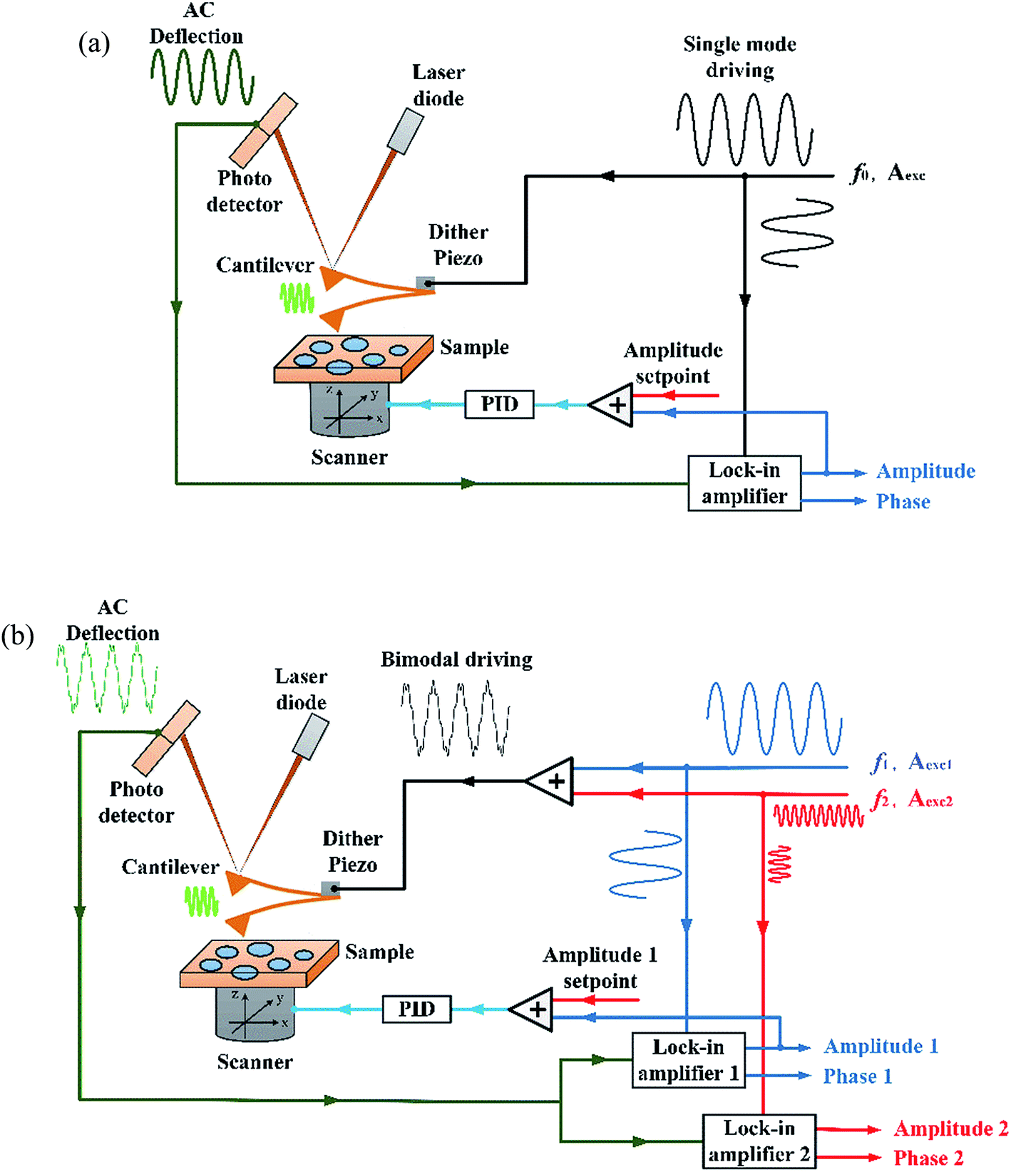 | ||
| Fig. 1 Control schemes of (a) single mode and (b) bimodal imaging in Cypher AFM equipment. | ||
3. Results and discussion
2.5 μm × 2.5 μm sample area which contains PS and LDPE regions was scanned by single and bimodal imaging modes. In single mode, phase shift signal could be measured and recorded with different setpoint for different free amplitudes (A01, A02, A03) based on Fig. 1(a). In bimodal mode, extra driving signal provides two additional response signals. Therefore, Ø1 (phase of the first mode), A2 (scanning amplitude of the second mode) and Ø2 (phase of the second mode) response signals could be measured and recorded based on Fig. 1(b). When the second driving signal was in the third resonant frequency, A2 and Ø2 would be instead by A3 (scanning amplitude of the third mode) and Ø3 (phase of the third mode). Fig. 2 shows response signals of bimodal imaging on a selected PS-LDPE area, (a) height, (b) A2, (c) Ø1 and (d) Ø2.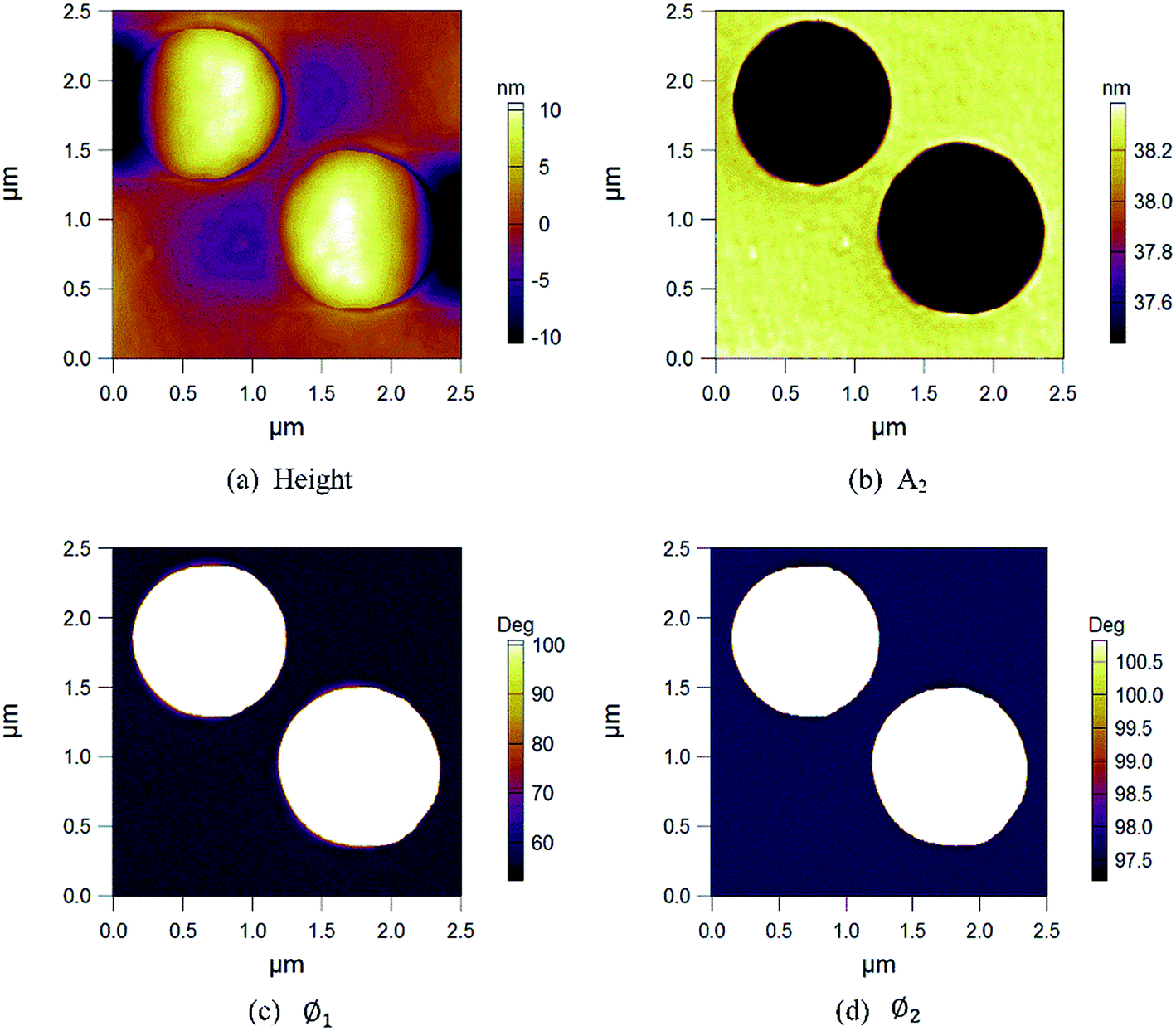 | ||
| Fig. 2 Response signals of bimodal imaging (a) height, (b) A2, (c) Ø1 and (d) Ø2. The amplitude and the phase images are in nm and degrees, respectively. | ||
3.1. Single imaging
Phase might lie above or below 90 degrees which defines two distinct force regimes in standard AM-AFM. Two regimes are attractive regime (net attractive force) and repulsive regime (net repulsive force), respectively. Fig. 3 displays the phase shift curves on PS and LDPE regions for the first, second and third resonance frequency modes respectively. In Fig. 3(a), the phase shift values of PS and LDPE in the first mode are all above 90 degrees when the free amplitude A01 = 20 nm, 30 nm and 40 nm. Therefore, it can be considered that the tip scanned in the net attractive mode. Obviously, the phase shift of PS and LDPE both change bigger with the increase of free amplitude and the decrease of setpoint. In Fig. 3(b), the phase shift curves of PS and LDPE in the second mode show a process of first increase and then decrease when the setpoint lower gradually. It indicates that the tip goes through the attractive force regime (setpoint ratio mainly from 0.25–0.9) and reach the repulsive force regime (setpoint ratio mainly from 0.05–0.25). Lower turning points about 0.1 occur in the phase curves of A02 = 40 nm. That is because great free amplitudes might help the tip escape from the adsorption range. Fig. 3(c) shows the phase shift curves of PS and LDPE in the third mode. Phase shift of different curves drop below 90 degrees when the setpoint ratio varies between 0.4–0.75. When free amplitude A03 > 40 nm was chosen, the polymers always were destroyed in experiments. Therefore, A03 = 20 nm, 30 nm and 40 nm were properly chosen in the third mode. Clearly, it has a shorter range of attractive regime when the cantilever is driven by higher mode under the same free amplitude. | ||
| Fig. 3 (a) Phase Ø1, (b) phase Ø2 and (c) phase Ø3 of single modes are summarized with different A01, A02 and A03. The amplitude and the phase images are in nm and degrees, respectively. | ||
The amplitude and phase signals can be converted into dissipated power and virial which are closely related to the non-conservative and conservative tip-sample interactions across the sample, respectively. Fig. 4(a)–(c) display the dissipated power curves in PS and LDPE regions with different free amplitudes for the first, second and third modes, respectively. In Fig. 4(a), dissipated power in PS and LDPE regions show half a parabolic monotone increasing trends with the increase of setpoint ratio for all free amplitudes A01. In addition, the power in LDPE region dissipates significantly more than that in PS region for the same A01. Fig. 4(b) shows the dissipated power curves in PS and LDPE regions for all free amplitudes A02. The parabolic shape dissipation curves display crossing phenomenon between PS and LDPE which are different from the first mode. The power in PS region dissipates significantly more than that in LDPE region during the middle range of setpoint when the A02 = 40 nm. On the contrary, dissipated power in PS region is a little bit small than that in LDPE region when the A02 = 30 nm and 20 nm. Fig. 4(c) depicts dissipated power curves in PS and LDPE regions for all free amplitudes A03. Parabolic curves of PS and LDPE for the same free amplitude A03 are rather close. Obviously, higher modes correspond to greater power dissipation because of higher resonance frequencies and larger spring constants.
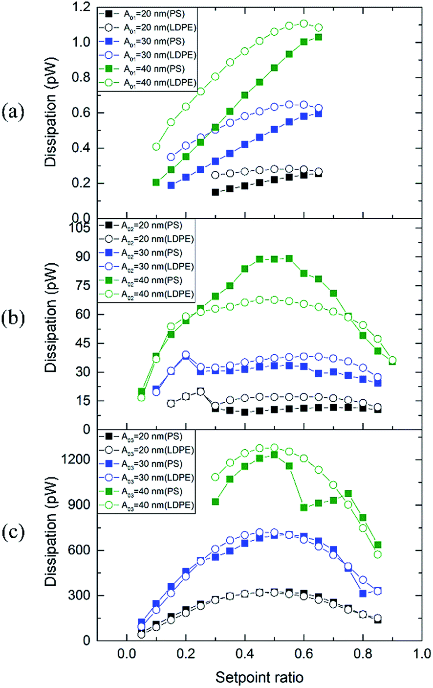 | ||
| Fig. 4 Dissipated power measured on PS-LDPE with different free amplitudes A0. (a) First mode, (b) second mode, and (c) third mode. | ||
Fig. 5 displays the corresponding virial curves in PS and LDPE regions for Fig. 3. The sign of virial might take positive or negative values because of the cosine value of phase. In Fig. 5(a), the first mode virial curves of PS-LDPE remain parabolic shape. Greater free amplitudes of A01 show more virial. Virial values in PS regions are larger than that in LDPE region for the same A01. In Fig. 5(b), the virial becomes negative when the setpoint ratios are rather low in the second mode. It agrees with that greater amplitudes or high modes lead to contact or greater penetration into the sample which in turn results in greater repulsive forces. The values of virial are −2.12 to 38.9 aJ (PS) and −4.7 to 45.1 aJ (LDPE) for A02 = 40 nm. In Fig. 5(c), the virial becomes more negative on a large scale of setpoint ratio in the third mode. Therefore, greater repulsive force often occur in higher mode, which might damage soft samples.
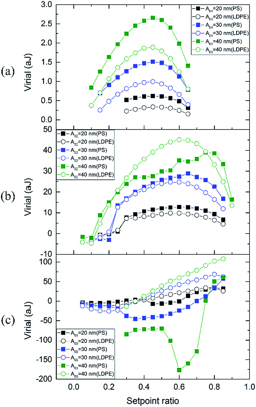 | ||
| Fig. 5 Virial measured on PS-LDPE with different free amplitudes A0 for three single modes. (a) First mode, (b) second mode and (c) third mode. | ||
Significant phase contrast differences can be observed qualitatively by operating in repulsive regime of AM-AFM mode. The methods described in some literatures have been used extensively in mapping relative differences between various regions of a multi-component sample. Higher single mode and bimodal mode response signals are quantitatively converted to contrast in this article which is beneficial to optimize the imaging conditions in experiments. Fig. 6 displays phase contrast curves of first, second and third modes, respectively. In Fig. 6(a), contrast of phase Ø1 for A01 = 20 nm, 30 nm and 40 nm present parabolic shapes. Greater free amplitudes show better contrast and the best one is 10.95 where A01 is 40 nm and setpoint ratio is 0.25. In Fig. 6(b), contrast values of phase Ø2 are relatively high for A02 = 20 nm and the best contrast is 9.76 where the setpoint ratio is 0.65. In Fig. 6(c), better contrast of phase Ø3 for different A03 are shown at low setpoint ratios. The best contrast among three modes is 20.3 when the setpoint ratio is 0.10 of A03 = 20 nm. Therefore, same or even better contrast can be obtained in high modes with small free amplitudes.
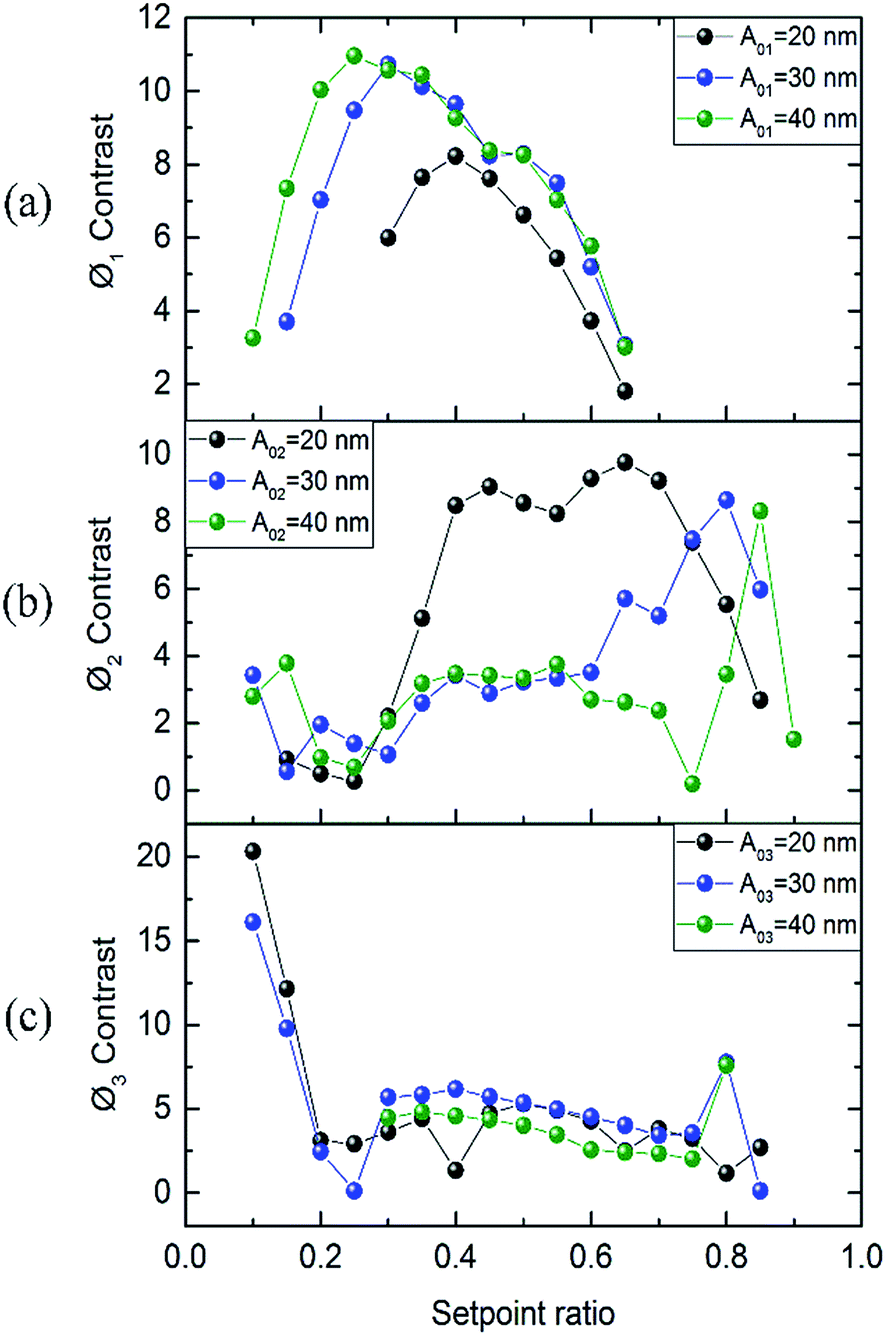 | ||
| Fig. 6 Phase contrasts of different free amplitude A0 for three single modes, respectively. (a) First mode, (b) second mode, (c) third mode. | ||
3.2. Bimodal imaging
Phase of bimodal mode with different free amplitude A01 and A02 (A01 and A03) were also recorded. Free amplitude of the first flexural mode A01 is a crucial parameter which may determine the interaction force regime. The second (third) flexural mode free amplitude A02 (A03) varied sequentially in a small interval over the course of a specific free amplitude A01. Unlike other reports, a wide range of A02 (A03) values were chosen to drive the cantilever along with A01. The optional non-destructive ranges of the free amplitude for A02 (A03) were 1.2–49.4 nm (0.48–20 nm) which may not damage the microstructure of the sample. According to the principle of control shown in Fig. 1(b), two phase signals both can be collected dynamically in bimodal imaging mode. The setpoint ratio of the first mode amplitude was ∼0.5 which can ensure imaging from attractive regime to repulsive regime. The phase of the first mode Ø1 and the second mode Ø2 (third mode Ø3) curves obtained in the bimodal scanning process are shown in Fig. 7. Fig. 7 summarizes the changes of phase values in PS and LDPE regions with different free amplitudes A01 and A02 (A03). Fig. 4(a) and (b) are Ø1 and Ø2 curves when the cantilever was driven by the first and second flexural modes, and the Fig. 4(c) and (d) are Ø1 and Ø3 results when the bimodal signals are in the first and third flexural modes. In Fig. 7(a), Ø1 curves present a trend of monotone increasing in LDPE region and a trend of first increase and then decrease on PS region with the gradually increasing of A02 from 1.2–49.4 nm. Almost all phase points on the curves are above 90 degrees which corresponds to attractive mode. In Fig. 7(b), Ø2 curves show a trend of first increase and then decrease both in PS and LDPE regions with the gradually increasing of A02. Values of Ø2 are all above 90 degrees. Fig. 7(c) and (d) respectively show Ø1 and Ø3 curves where the bimodal signals are the first and third modes. The trends of the Ø1 and Ø3 curves are similar to the trends of Ø1 and Ø2 in Fig. 7(a) and (b). The difference is that the range of A03 is from 0.48 nm to 20 nm. Because of the dynamic spring constant of the third mode is quite large which makes the tip harder and easily break through the attractive regime with comparatively small amplitudes.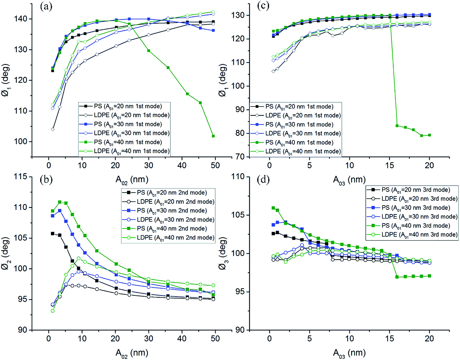 | ||
| Fig. 7 (a) Phase Ø1 and (b) phase Ø2 with different A01, A02 for bimodal of the first and second modes; (c) phase Ø1 and (d) phase Ø3 with different A01, A03 for bimodal of the first and third modes. | ||
Similarly, the interfacial interactions between probe tip and PS-LDPE are also investigated for bimodal mode. Dissipated power curves of PS and LDPE in bimodal mode are displayed in Fig. 8 with different free amplitudes for each mode. Fig. 8(a) and (b) are the dissipation curves of the first mode and the second mode versus varying free amplitudes of the second mode A02 (1.2–49.4 nm) and (c), (d) are the dissipation of the first mode and the third mode versus A03 (0.48–20 nm), respectively. The trends of PS and LDPE dissipation curves in Fig. 8(a) are contrary to those of the first mode phase in Fig. 7(a). Fig. 8(b) shows consistent exponential growth curves of PS-LDPE dissipation for all A01. Maximum values of dissipated power are about 68 pW at A02 = 49.4 nm, and minimum values of dissipated power are about 0.07 pW at A02 = 1.2 nm. In Fig. 8(c), greater free amplitude A01 corresponds to more dissipated power both in PS and LDPE regions clearly. In Fig. 8(d), the maximum values of dissipated power are about 108–126 pW at A03 = 20 nm, and minimum values of dissipated power are about 0.07 pW at A03 = 0.48 nm for all three A01. Therefore, dissipated power of the first mode (∼2.0 pW) is obviously much smaller than that of the second mode (∼68 pW) and the third mode (∼126 pW).
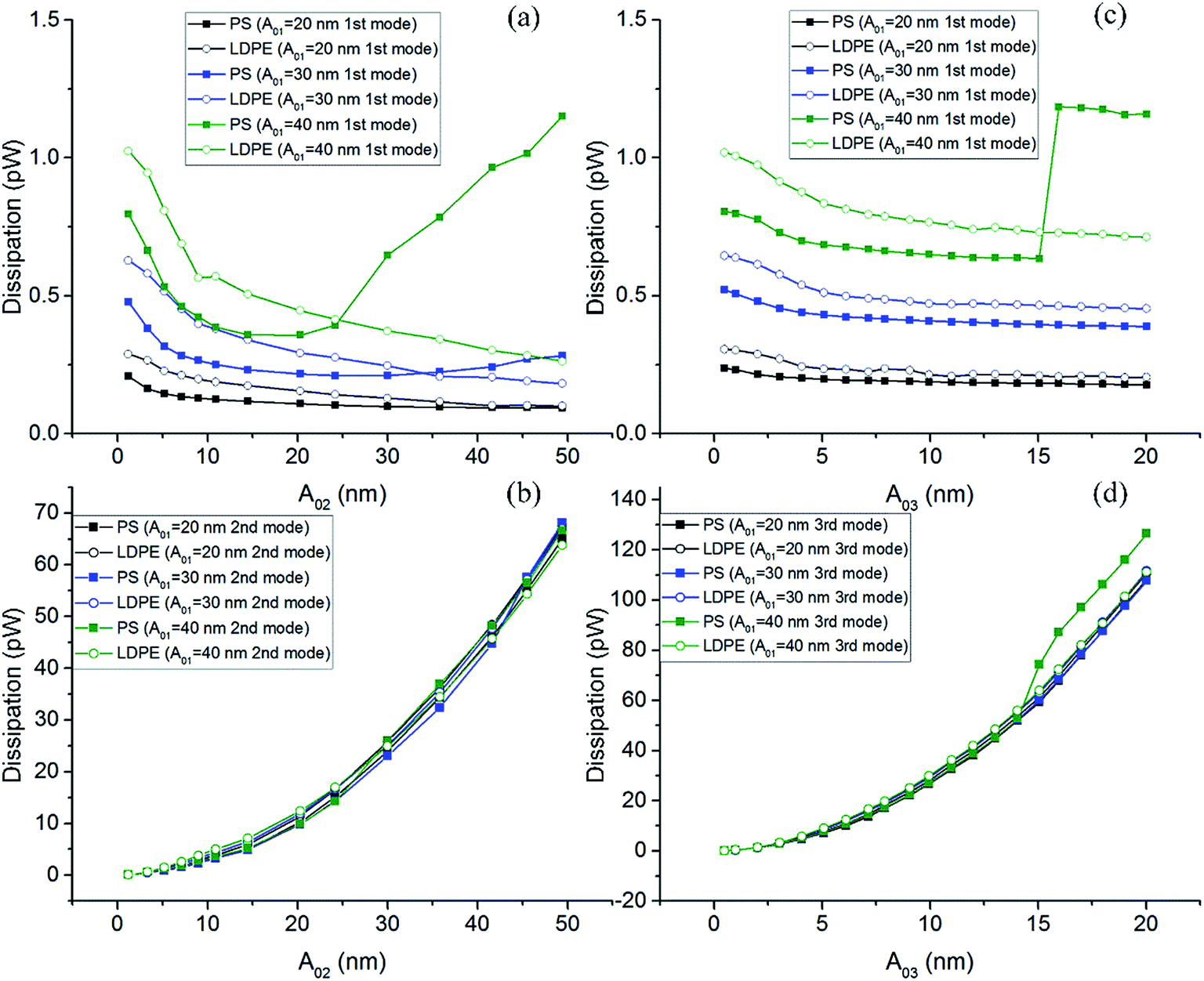 | ||
| Fig. 8 Dissipated power measured on PS-LDPE in bimodal mode with different free amplitudes A0. (a) and (b) are the dissipation curves of the first mode and the second mode for different A01 (20 nm, 30 nm, 40 nm) versus varying A02 (1.2–49.4 nm); and (c), (d) are the dissipation curves of the first mode and the third mode for different A01 (20 nm, 30 nm and 40 nm) versus varying A03 (0.48–20 nm). | ||
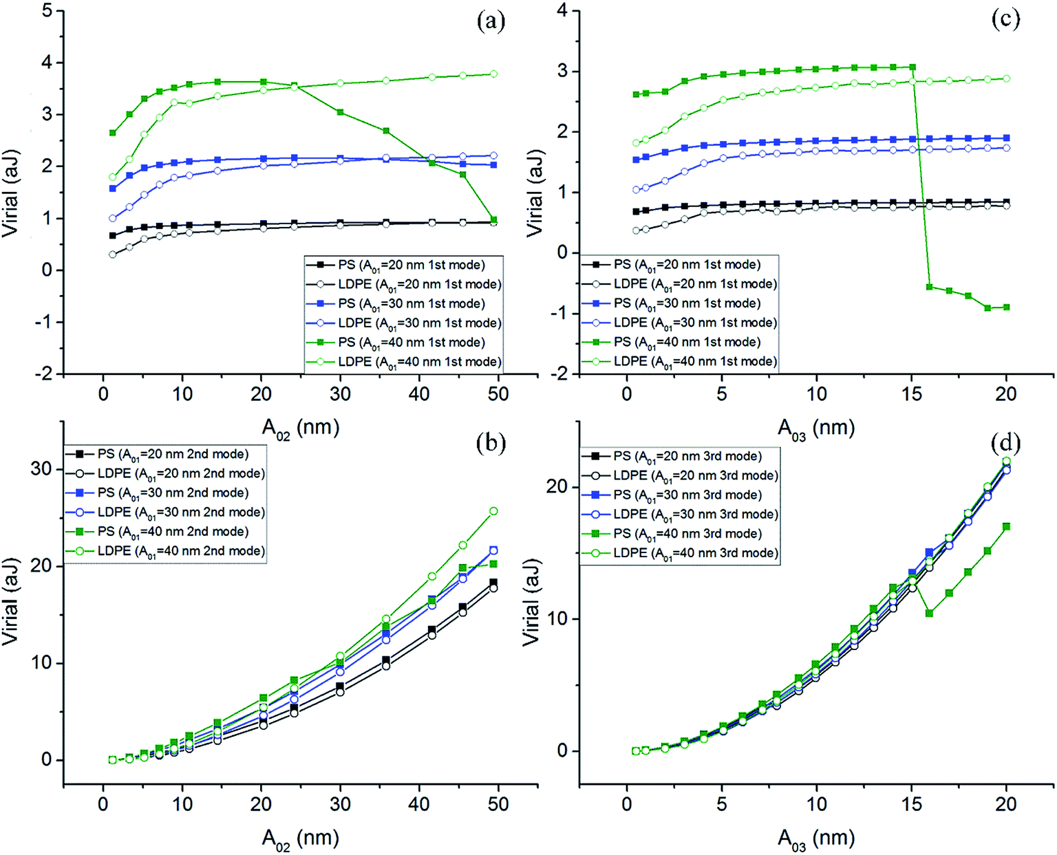
Virial of bimodal images are also calculated to analysis the energy transfer in the presence of conservative and dissipative interactions of multi modes. Fig. 9 shows the virial curves plotted from two type bimodal modes. In Fig. 9(a) and (c), the virial trends of first mode just like that in Fig. 7(a) and (c), respectively. Greater free amplitudes corresponding to higher virial values in LDPE region. Different from small free amplitudes of A02 and A03, virial decrease for A01 = 40 nm during greater A02 and A03 in PS region. Fig. 9(b) and (d) both display half a parabolic monotone increasing trends with the increase of A02 and A03.
 | ||
| Fig. 9 Virial measured on PS-LDPE in bimodal mode with different free amplitudes. Bimodal of first and second modes: (a) and (b) are the virial curves of the first mode and the second mode for different A01 (20 nm, 30 nm, 40 nm) versus varying A02 (1.2–49.4 nm); and bimodal of first and third modes: (c) and (d) are the virial curves of the first mode and the third mode for different A01 (20 nm, 30 nm, 40 nm) versus varying A03 (0.48–20 nm). | ||
Contrast of bimodal response signals are also calculated and plotted in Fig. 10. For combination of first and second modes or first and third modes, there are three signals, A2, Ø1 and Ø2 (A3, Ø1 and Ø3) for determined bimodal mode which can present material components and properties. These three signals can be employed to image the surface topography, especially the contrasts of component material. Fig. 10(a) and (e) show the imaging schematics of two types bimodal mode in our experiments. In Fig. 10(b), curves show relatively better contrasts of A2 when A02 is during 10–30 nm. In Fig. 10(c) and (d), curves show relatively better contrasts when A02 is during 1–10 nm. The highest contrast value for this bimodal mode is 12.8 when the free amplitude of the first mode and second mode are 40 nm and 5 nm, respectively. While beyond that, PS and LDPE almost can not be distinguished by Ø1 and Ø2 images because of D < 2. In Fig. 10(f), curves show relatively better contrasts of A3 when A03 is during 5–17.5 nm. In Fig. 10(g) and (h), contrast curves of Ø1 and Ø3 are all above D = 2. Greater free amplitude A01 shows higher contrast values. Small free amplitude A03 (0.48–3 nm) present better contrast for Ø1 and Ø3. It is important to note that greater A03 also reflects enough potential to obtain enhanced contrast which is superior to bimodal combination of the first and second modes. The maximum contrast values of bimodal modes are summarized in Table 1. It suggests that bimodal excitation of great free amplitude A01 and small free amplitude A03 might obtain the best phase image contrasts in experiments.
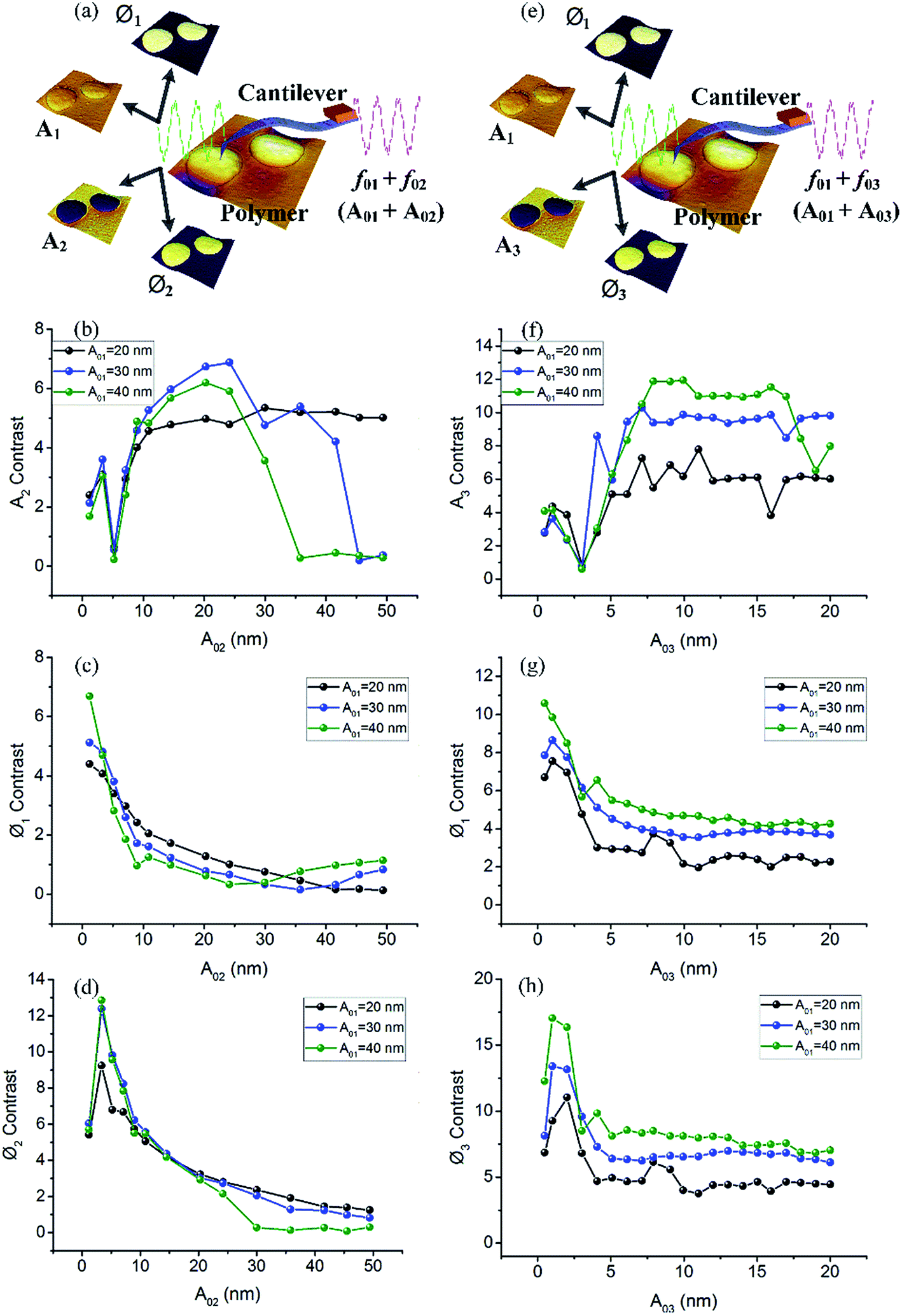 | ||
| Fig. 10 Amplitude and phase contrast curves of different free amplitudes A01 and A02 (A03) for two types bimodal modes. Bimodal of first and second modes: (a) imaging schematic, (b) A2 contrast, (c) Ø1 contrast and (d) Ø2 contrast; bimodal of first and third modes: (e) imaging schematic, (f) A3 contrast, (g) Ø1 contrast and (h) Ø3 contrast. | ||
| A01 (nm) | 20 | 30 | 40 |
| D(A2)max | 5.34 | 6.87 | 5.77 |
| D(Ø1)max | 4.39 | 5.12 | 6.69 |
| D(Ø2)max | 9.24 | 12.4 | 12.8 |
| D(A3)max | 7.79 | 10.3 | 11.9 |
| D(Ø1)max | 7.54 | 8.63 | 10.6 |
| D(Ø3)max | 11.0 | 13.4 | 17.0 |
4. Conclusions
Single mode and bimodal AFM experiments have been conducted on a PS-LDPE polymer blend with different free amplitudes by cantilever AC240. Results show that tip-sample interfacial interaction of greater free amplitudes correspond to more dissipated power and virial value in single mode. Higher single modes might dissipate more power than that of the first mode. Greater free amplitudes usually produce better contrasts for the first single mode. However, small free amplitudes in higher single modes (the second and third) show the potential to obtain enhanced contrast. The best image contrast of single mode appears in the third mode scanning. In bimodal mode, phase contrast of higher mode shows distinct advantages in comparison to phase and amplitude of the first mode. Moreover, combination of the first two modes can only be used to distinguish materials within small free amplitude (0–10 nm) of the second mode. Nevertheless, combination of the first and the third modes present more enhanced contrast within the whole free amplitude range (0–20 nm) of the third mode. Interestingly, greater free amplitudes of the first mode obviously contribute to improve the overall contrast in bimodal mode. The best contrast of bimodal imaging occurs when the first and third free amplitude are relative great and small, respectively. In addition, bimodal imaging (especially the third mode adds to the first mode) shows more advanced and stable amplitude and phase images than those in single higher mode. Research of higher mode and bimodal AFM imaging might be of great help to improve contrast and quantitative analysis of material properties.Conflicts of interest
There are no conflicts to declare.Acknowledgements
We thank Asylum Research engineers for helpful discussions. This research is financially supported by the National Natural Science Foundation of China (Grant No. 51527901 and 51375255).References
- Y. Martin, C. C. Williams and H. K. Wickramasinghe, J. Appl. Phys., 1987, 61, 4723–4729 CrossRef CAS.
- Q. Zhong, D. Imniss, K. Kjoller and V. B. Elings, Surf. Sci., 1993, 290, L688 CrossRef CAS.
- R. W. Stark, T. Drobek and W. M. Heckl, Appl. Phys. Lett., 1999, 74, 3296–3298 CrossRef CAS.
- O. Pfeiffer, C. Loppacher, C. Wattinger, M. Bammerlin, U. Gysin, M. Guggisberg, S. Rast, R. Bennewitz, E. Meyer and H. J. Guntherodt, Appl. Surf. Sci., 2000, 157, 337–342 CrossRef CAS.
- Y. Sugimoto, S. Innami, M. Abe, O. Custance and S. Morita, Appl. Phys. Lett., 2007, 91, 093120 CrossRef.
- R. C. Tung, T. Wutscher, D. Martinez-Martin, R. G. Reifenberger, F. Giessibl and A. Raman, J. Appl. Phys., 2010, 107, 104508 CrossRef.
- R. Garcia and E. T. Herruzo, Nat. Nanotechnol., 2012, 7, 217–226 CrossRef CAS PubMed.
- J. R. Lozano and R. Garcia, Phys. Rev. Lett., 2008, 100, 076102 CrossRef PubMed.
- R. Proksch, Appl. Phys. Lett., 2006, 89, 113121 CrossRef.
- S. Jesse, S. V. Kalinin, R. Proksch, A. P. Baddorf and B. J. Rodriguez, Nanotechnology, 2007, 18, 435503 CrossRef.
- T. Rodriguez and R. Garcia, Appl. Phys. Lett., 2004, 84, 449–451 CrossRef CAS.
- S. Santos, Appl. Phys. Lett., 2013, 103, 231603 CrossRef.
- N. F. Martinez, J. Lozano, E. T. Herruzo, F. Garcia, C. Richter, T. Sulzbach and R. Garcia, Nanotechnology, 2008, 19, 384011 CrossRef CAS PubMed.
- A. M. Gigler, C. Dietz, M. Baumann, N. F. Martinez, R. Garcia and R. W. Stark, Repulsive bimodal atomic force microscopy on polymers, Beilstein J. Nanotechnol., 2012, 3, 456–463 CrossRef CAS PubMed.
- A. Berquand, P. E. Mazeran and J. M. Laval, Surf. Sci., 2003, 523, 125–130 CrossRef CAS.
- C. Sommerhalter, T. W. Matthes, T. Glatzel, A. Jager-Waldau and M. C. Lux-Steiner, Appl. Phys. Lett., 1999, 75, 286–288 CrossRef CAS.
- I. Chakraborty and D. G. Yablon, Nanotechnology, 2013, 24, 475706 CrossRef PubMed.
- S. Santos, Appl. Phys. Lett., 2014, 104, 143109 CrossRef.
- R. W. Stark, Appl. Phys. Lett., 2009, 94, 063109 CrossRef.
- S. An, S. D. Solares, S. Santos and D. Ebeling, Nanotechnology, 2014, 25, 475701 CrossRef PubMed.
- J. Tamayo and R. Garcia, Appl. Phys. Lett., 1998, 73, 2926–2928 CrossRef CAS.
- A. J. Diaz, B. Eslami, E. A. López-Guerra and S. D. Solares, J. Appl. Phys., 2014, 116, 104901 CrossRef.
- G. Chawla and S. D. Solares, Appl. Phys. Lett., 2011, 99, 074103 CrossRef.
- R. Garcia, J. Tamayo and A. S. Paulo, Surf. Interface Anal., 1999, 27, 312–316 CrossRef CAS.
- J. P. Cleveland, B. Anczykowski, A. E. Schmid and V. B. Elings, Appl. Phys. Lett., 1998, 72, 2613–2615 CrossRef CAS.
- J. Lozano and R. Garcia, Phys. Rev. B: Condens. Matter Mater. Phys., 2009, 79, 014110 CrossRef.
- D. Forchheimer, R. Forchheimer and D. B. Haviland, Nat. Commun., 2015, 6, 6270 CrossRef CAS PubMed.
- K. M. Ashman, C. M. Bird and S. E. Zepf, Astron. J., 1994, 108, 2348–2361 CrossRef.
- S. Shi, D. Guo and J. B. Luo, RSC Adv., 2017, 7, 11768–11776 RSC.
- D. Kiracofe and A. Raman, Nanotechnology, 2011, 22, 485502 CrossRef PubMed.
- R. Garcia and S. Paulo, Phys. Rev. B: Condens. Matter Mater. Phys., 1999, 60, 4961–4966 CrossRef CAS.
| This journal is © The Royal Society of Chemistry 2017 |