An unmodified graphene foam chemical sensor based on SVM for discrimination of chemical molecules with broad selectivity

Abstract

Compared to conventional chemical sensors, this paper presented a chemical sensor system with broad selectivity for a variety of molecules without any surface modification. The system consisted of an unmodified graphene foam as sensing element, an electrical resistance time domain detection system and a Support Vector Machine (SVM) identification system. The chemical sensor adopted 3D graphene foam to increase the reaction area and improve the sensitivity for detecting target molecules. The electrical resistance time domain detection system was constructed to record the graphene resistance curve in real time with different molecules. Based on the diverse shapes of the electrical resistance curves, SVM was used to extract features of each resistance curve and discriminate the corresponding molecules via pattern recognition of each resistance curve without any graphene modification. As validation experiments, six kinds of chemical molecules (chloroform, acetone, ether, toluene, ethyl benzene and methanol) have been tested. The discrimination accuracy for each molecule could be above 98% which showed a broad selectivity for a variety of molecules. Furthermore, through theoretical calculation with the first principle, we concluded that different band structures of the graphene caused by different molecules were the mechanism for the graphene chemical sensor system to discriminate chemical molecules with selectivity. This work may present a new strategy for research and application for graphene chemical sensors.

---

1. Introduction

Graphene, composed of carbon atoms arranged in a honeycomb lattice, has attracted widespread attention due to its high surface-to-volume ratio, two-dimensional structure, and excellent electrical, optical and mechanical properties.^1–4 Owing to these characteristics of graphene, numerous chemiresistors,^5–7 field-effect transistors^8,9 and other chemical sensors based on graphene have been studied and reported.^10,11 Our group also has done some research on graphene materials and graphene sensors including graphene preparation,¹² graphene FET,¹³ graphene pH sensors¹⁴ and graphene SPR sensors.¹⁵

Selectivity is one of the fundamental characteristics of sensors. In order to construct graphene sensors with selectivity, most bio-chemical sensors need to perform surface modification of graphene, including doping with some elements or attaching chemical groups, metal nanoparticles,^16,17 enzymes or biomolecules polymers etc.^18,19 Therefore, surface modification is a common strategy to fabricate a bio-chemical sensor with selectivity. However, through theoretical simulation of the interaction between molecules and graphene, some researchers have found that interactions between molecules and graphene have different effects on the electrical properties of graphene, which may have provided a theoretical support for fabricating unmodified graphene sensors with selectivity.^20–22 Without any surface modification, Dobrokhotov et al. reported a vapor chemiresistor for recognition of acetone, ethanol, and toluene, which processed the response data of chemiresistor with a fast Fourier transform and quadratic discriminant analysis.²³ Rumyantsev et al. reported a graphene transistor which used low frequency noise spectra as an additional sensing parameter to enhance selectivity for gas sensing.^24,25 Eric C. Nallon et al. fabricated a chemical vapor sensor which utilized Principle Component Analysis (PCA) to obtain selectivity for a variety of molecules.²⁶ In order to increase active surface area and improve the sensitivity, the chemical vapor sensors were created by performing standard photolithography to define interdigitated electrode contacts which increased the difficulty for sensor design in some degree.

Since a porous carbon network has the same excellent performance as two-dimensional graphene, 3D graphene foam is the perfect morphology to increase the active surface area and has also been attractive for chemical or biological sensor design.^27,28 Meanwhile, considering the resistance measurement is a simple but effective method in chemiresistor research,²⁹ we have constructed a graphene chemical sensor (GCS) system consisting of an unmodified 3D graphene foam as the sensing element and an electrical resistance time domain detecting system (ERTDS) to record the GCS resistance response curve for a variety chemical molecules including chloroform, ether, acetone, methanol, toluene and ethyl benzene. Based on diverse shape of response curves, support vector machine (SVM),^30–33 a kind of pattern recognition method was used to classify the resistance curves and subsequently discriminate target molecules with selectivity. Since different molecules could induce different resistance curves, the GCS system has demonstrated desirable capability for discrimination of target chemical molecules with broad selectivity. The results have also exhibited other advantages such as simple operation, low cost, rapid response and recovery and high reproducibility.

2. Experimental section

2.1 Materials and apparatus

Three dimension graphene foam with size of 50 mm × 50 mm was purchased from 6Carbon Technology (Shenzhen, China). Glass substrate with indium tin oxide (ITO) electrodes as a substrate for GCS was purchased from Hua Nan Xiang Cheng Ltd. (Shenzhen, China). Silver conductive paint was purchased from CAIG Laboratories Inc. (CW-200, USA). Chloroform, ether, acetone, methanol, toluene and ethyl benzene are all analytical grade.

The 3D graphene foam characterization was carried out by a confocal Raman microscopy (SPEX-1403, SPEX). The morphologies of the 3D graphene were characterized by scanning electron microscopy (SEM, FEI Nova Nano450). A homemade ERTDS was used to record the graphene resistance curve in real time. With reference to the previous work,²³ we designed a vapor generation system (VGS) to generate analytic molecules. All the experiments were carried out at experimental room conditions.

2.2 Fabrication of GCSs and VGS

The GCSs were designed by 3D graphene foam as shown in Fig. 1.

Fig. 1 Fabrication of 3D graphene foam and electrical resistance time domain detection system (SCP: silver conductive paint, CCS: constant current source, IA: instrument amplifier, MCU: micro control unit, TD: targets discrimination).

The graphene foam was prepared by typical chemical vapor deposition (CVD) on foam nickel substrate.^34–36 In briefly, graphene films were precipitated on the surface of the nickel foam by CVD method. The nickel skeleton was etched away by FeCl₃ after a thin layer of poly(methyl methacrylate) (PMMA) was deposited on the surface of the graphene films as a support. Finally, the PMMA support was removed by hot acetone to obtain 3D graphene foam. Glass substrate with ITO electrodes was cleaned for 5 minutes by ultrasonic wave in deionized water. The size of the glass substrate was 20 mm × 10 mm and the size of each ITO electrode was 20 mm × 2 mm. A piece of graphene foam with size of 10 mm × 5 mm was adhered on the ITO electrodes by silver conductive paint. Drying for 12 hours at room temperature, the silver conductive paint was solidified and the GCS was completed for measurement.

The designed VGS was shown in Fig. 2. The organic solvent was injected into the vapor generate chamber through a precision syringe and heated to a gaseous state by a heating plate. The temperature of the heater was set at 40 °C and the volume of the chamber was about 200 mL. Therefore, with 100 μL of the organic solvent added to the chamber, the vapor concentration could be estimated to be 100–200 ppm based on mass concentration. The concentration of the detection vapor could be changed by controlling the volume of the solvent added to the vapor generate chamber. Combined with two check valves, the miniature pump pumped the analytic molecules gas into the sensing chamber. The ERTDS recorded the electrical resistance of the sensor in real time.

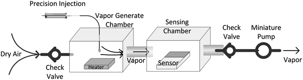Fig. 2 Structure of the vapour generation system.

2.3 Electrical resistance time domain detection system

The adsorption and desorption of molecules on the interface of graphene could change the electrical resistance of the graphene.²⁹ An ERTDS was constructed to detect the electrical resistance of the GCS. Since graphene foam has its intrinsic electrical resistance and tiny fluctuant resistance would generated by adsorption and desorption of molecules on the interface of graphene, a Wheatstone bridge circuit and an instrument amplifier were utilized to amplify the tiny fluctuant resistance (ΔR) of GCSs to a voltage signal as shown in Fig. 1. The amplified voltage signal was converted to digital signal collected by an analog-to-digital (A/D) conversion module and acquired by a micro control unit. In order to extract features of the GCSs resistance correctly, the precision of the A/D module was 12 bit and the sampling speed of the A/D module was more than 1 kbit per s. For each experiment, the intrinsic resistance of the GCS was recorded firstly as baseline. When a kind of chemical molecule was absorbed onto the GCS surface, the real-time resistance curve of GCSs was recorded by the ERTDS and uploaded to a computer via an USB interface.

2.4 Targets discrimination algorithm

The real-time resistance curve was used for targets discrimination based on pattern recognition. The algorithm for chemical targets discrimination is composed of Data Preprocessing (DPP), Machine Learning (ML) and Targets Identification (TI) as shown in Scheme 1.

Scheme 1 Targets discrimination algorithm for GCS system.

2.4.1 Data preprocessing. DPP was utilized to obtain normalized feature vectors from the resistance curve of the GCS. For training samples (step 1), the extracted feature vectors were normalized to generate a hyperplane model by machine learning module (step 2). For predicating targets, the feature vectors were also extracted and normalized to obtain predication vectors (step 3). Feature vectors extraction is key process of selecting a subset of features for model construction. A typical resistance curve R(t) of GCS response for chemical molecule was shown in Fig. 3.

Fig. 3 Typical GCS resistance response curve of R(t) and extraction of features. (a) Features of R_max, T_A, R_avg, T_rec, T_res, A_res. (b) Enlarged view of region I in (a) indicating S_A. (c) Enlarged view of region II in (a) indicating S_D.

In Fig. 3(a), baseline represented the graphene resistance without chemical samples. For the purpose of making the feature extraction standardization, each resistance value of GCSs has been normalized through normalizing the baseline average to zero. Therefore, the y-axis represented relative resistance of GCSs in Fig. 3. At the “Add sample” point, chemical sample was dropped on the surface of graphene foam. The resistance of GCS ascended quickly and then recovered to a stable value. The first data point, after which the variance of the consecutive 100 data points was less than 1, was regarded as the “End point” of the whole reaction. For each resistance curve, the following features were extracted to form a feature vector (S_A, R_max, T_A, R_avg, S_D, T_rec, T_res, A_res). S_A indicates the ascending speed of the GCSs to chemical samples. It was obtained by calculating the slope between the third data point after “Add sample” as shown in Fig. 3(b). R_max is the difference between the maximum relative resistance value and the average resistance of the baseline. T_A is ascending time from “Add sample” point to maximum relative resistance point. R_avg is average resistance during ascending time. S_D means descending speed as shown in Fig. 3(c). T_rec is recovery time from maximum relative resistance point to “End point”. T_res is the whole response time from “Add sample” point to “End point”. A_res is the area of the whole response curve which was shown as gray area in Fig. 3(a).

2.4.2 Machine learning. ML is a field of scientific study that concentrates on iterative algorithms, which are operated to build a model from training data and using that model to make predictions for unseen samples. In this work, LIBSVM, a software package developed by professor Lin³⁷ was used to implement machine learning process. The main purpose of machine learning in this work is to find an optimal hyperplane model to distinguish different samples by using training vectors which have been obtained in DPP.

2.4.3 Targets identification. For prediction targets, feature vectors were also extracted firstly and normalized to form prediction vectors as described in DPP. The prediction vectors and the hyperplane model generated in ML were simultaneously inputted into a prediction function of SVM to export the predication results (step 4). The predication results could provide a probability distribution of one prediction target in all training samples.

3. Results and discussion

3.1 Characterization of 3D graphene foam

The morphology of the 3D graphene foam was characterized by a SEM (ZEISS, SUPRATM-55). As shown in Fig. 4(a), the graphene foam has exhibited an excellent 3D interconnected networks and macroporous structure with the pore diameter ∼200 to 300 μm which could offer a much larger specific surface area than 2D graphene films. In addition, the thin graphene scaffold contained many ripples and wrinkles on its surface due to CVD growth on nickel substrate, which further increased the specific surface area of graphene. The Raman spectrum of 3D graphene foam has been demonstrated in Fig. 4(b). The Raman spectra present two prominent characteristic peaks at 1584.9 and 2722.2 cm⁻¹ corresponding to the G and 2D band of graphene respectively. The intensity ratio of G and 2D band indicates that the graphene foam is composed of few layer graphene.

Fig. 4 Characterization of 3D graphene foam. (a) SEM image of 3D graphene foam. (b) Raman spectra of 3D graphene foam.

3.2 Time domain resistance measurement

The GCSs real-time response was investigated by measuring the fluctuant resistance via the constructed ERTDS upon exposure to 6 kinds of chemically diverse analytes: chloroform, acetone, ether, toluene, ethyl benzene and methanol as shown in Fig. 5.

Fig. 5 Time domain resistance curve of GCSs for different chemical molecules ((a) acetone, (b) chloroform, (c) ether, (d) methanol, (e) toluene and (f) ethyl benzene).

Notably, although the response curves of the GCSs to each samples showed diverse shapes, all the shapes shared a common characteristic, which is all of them have the ascending and then descending process. The ascending process may indicate adsorption reaction of chemical molecules on the interface of graphene and the descending process may result from desorption of molecules from graphene in consideration of volatility of the chemical molecules. Based on this common characteristic, the feature vectors (S_A, T_A, R_avg, R_max, S_D, T_rec, T_res, A_res) of each curve were extracted and the elements in each feature vector were divided into 3 groups: vector 1 (S_A, T_A, R_avg) reflected the ascending features, vector 2 (R_max, S_D, T_rec) were descending features and vector 3 (T_res, A_res, R_max) represented the overall characteristics of the reaction curves.

3.3 Classification accuracy

The GCSs system created a generalized model through machine learning with 156 sets of known data firstly as described previously in this paper. Then, unseen samples were measured and the model was used to predict their class by SVM method. Considering the adsorption and desorption process of molecules on graphene surface, we investigated the relationship between classification accuracy and interaction process of chemical molecules on graphene surface. Fig. 6(a) shows the classification results based on vector 1 (S_A, T_A, R_avg) which obtained during adsorption process of molecules and graphene. Fig. 6(b) has shown the classification results by vector 2 (R_max, S_D, T_rec) which reflected desorption process. Fig. 6(c) is predictive results via vector 3 (T_res, A_res, R_max).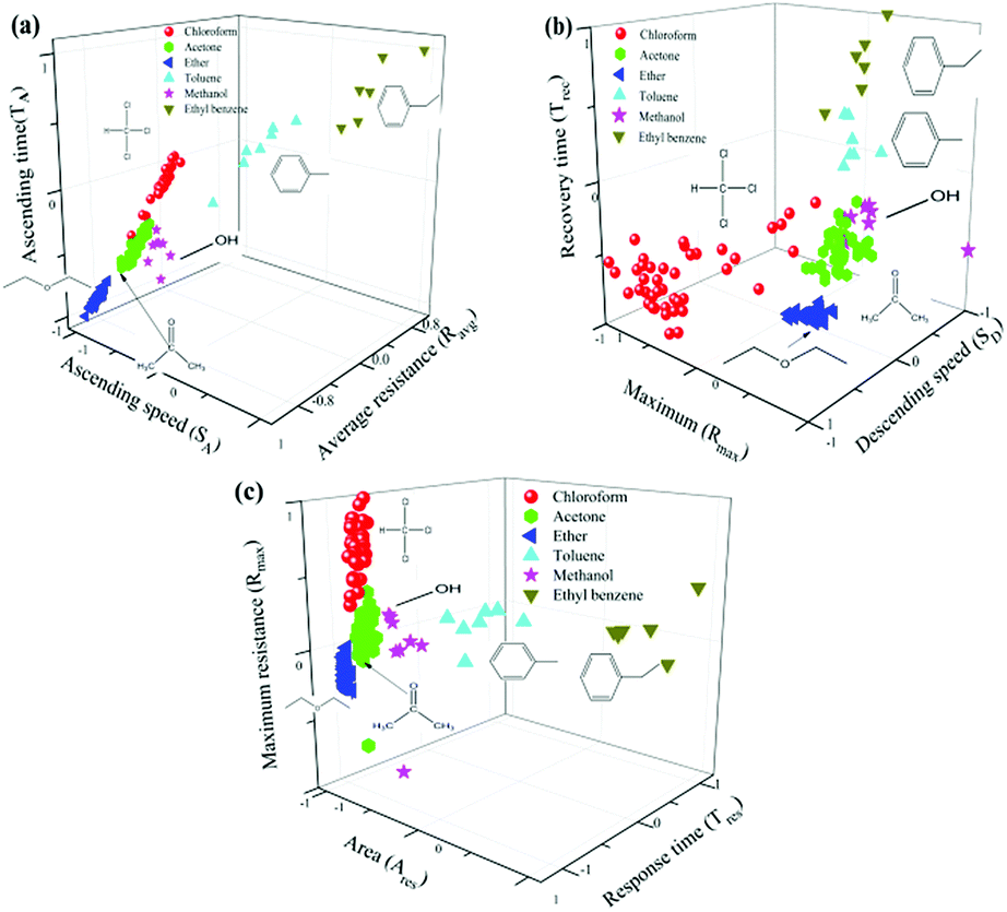

Fig. 6 Relationship between classification accuracy and subsets of feature vectors. (a) Classification results based on (S_A, T_A, R_avg). (b) Classification results based on (R_max, S_D, T_rec). (c) Classification results based on (R_max, T_res, A_res).

Firstly, it has been shown obviously from Fig. 6 that molecules with benzene ring structure including ethyl benzene and toluene can be easily separated from other molecules. Combined with time domain resistance curve in Fig. 6, it has also been demonstrated that benzene ring structure of molecules has obvious influence on the reaction time and the conductivity of the GCSs. We concluded this result was related with the π–π stack between benzene ring of molecules and six-member ring of graphene films.

Secondly, considering classification time is a very important parameter for GCSs system, we noted from Fig. 6 that only a subset of all features may identify target molecules, which make it feasible to shorten the detection time of GCSs and subsequently improve the classification speed. According to the feature emerging sequence during reaction process, we divided the reaction into four stages. Stage 1 represented the response speed of GCS to chemical molecules and only S_A could be obtained. At the end of stage 2 which meant the ascending process was finished (S_A, T_A, R_avg, R_max) could be generated. Stage 3 added feature of S_D which may reflect the desorption speed of molecules resulted from volatilization. Stage 4 represented that the reaction was finished and all the features could be obtained. Fig. 7(a) showed the predictive accuracy at each stage. It has been clearly demonstrated from Fig. 7(a) that the predictive accuracy was larger than 90% at the end of stage 2. Fig. 7(b) has given the predictive accuracy for each chemical molecule at stage 2 and stage 4 respectively. We can found from Fig. 7 that desired predictive accuracy could be achieved only through adsorption process of chemical molecules on graphene surface, which could reduce the classification time by about half according to the time domain resistant curves.

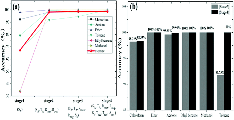Fig. 7 Comparison of prediction accuracy at different stage. (a) Classification accuracy at different stage during reaction. (b) Comparison of classification between stage 2 and stage 4.

Thirdly, we investigated the misjudgement rate for each chemical molecule as shown in Table 1. The most encountered misclassifications were chloroform as acetone, and toluene as ethyl benzene. From the time domain resistance curves in Fig. 5, it can be also found that the curve shapes of chloroform and acetone were similar, as well as the curve of toluene and ethyl benzene in ascending stage. We concluded that this misjudgement results were related with the molecule structure of the chemical molecules.

Table 1 Accuracy and misjudgment of predicted results of each chemical molecule

True samples	Stage	Accuracy (green) and misjudgement (red) of predicted results (%)
		Chloroform	Ether	Acetone	Toluene	Ethyl benzene	Methanol
Chloroform	Stage 2	98.22	0.02	1.76	0	0	0
	Stage 4	98.35	0.36	1.29	0	0	0
Ether	Stage 2	0	100	0	0	0	0
	Stage 4	0	100	0	0	0	0
Acetone	Stage 2	1.02	0.37	98.61	0	0	0
	Stage 4	0.085	0.005	99.91	0	0	0
Toluene	Stage 2	0	0	0	91.75	8.25	0
	Stage 4	0	0	0	100	0	0
Ethyl benzene	Stage 2	0	0	0	0	100	0
	Stage 4	0	0	0	0	100	0
Methanol	Stage 2	0	0	0	0	0	100
	Stage 4	0	0	0	0	0	100

---

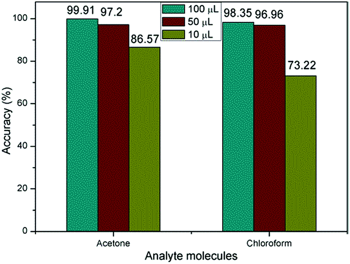
Finally, we investigate the relationship between classification accuracy and concentration of the analytic molecules. As described of the VGS, the concentration of the detection vapor could be changed by controlling the volume of the solvent added to the vapor generate chamber. When the volume of solvent added to the VGS was 100 μL, 50 μL and 10 μL, the concentration of the vapor could be estimated at about 150 ppm, 75 ppm and 15 ppm for acetone and chloroform. The corresponding response curves were shown in Fig. 8.

Fig. 8 Time domain resistance curve of GCSs for acetone and chloroform with different amount of solvent. (a) Acetone. (b) Chloroform.

As shown in Fig. 8, the resistance curves changed significantly as the concentration changes. However, the accuracy of identification was not significantly reduced until the concentration of analytic molecules was as low as 10 μL as shown in Fig. 9. This was due to the fact that the resistance curves of the various concentrations of the sample were used as training samples for machine learning, so that the recognition accuracy was kept high. However, when the sample concentration is very low, the error effect is more obvious than that of the high concentration samples, which leads to the decrease of recognition accuracy.

Fig. 9 Relationship between classification accuracy and concentration of molecules.

3.4 Discussion

In order to explain the mechanism for GCSs to discriminate chemical molecules with selectivity by time-domain resistance curves, we have tried to explore the interaction between chemical molecules and graphene by the first principle.^38,39 The system of chloroform molecule adsorbing on graphene surface was studied as an example. The effects of band structure and the adsorption distance to the conductive properties of graphene are discussed. All the calculations were performed by using Vienna Ab initio Simulation Package (VASP) with the projector augmented wave (PAW) basis sets.^40,41 The generalized gradient approximation (GGA) with the Perdew–Burke–Ernzerhof (PBE) exchange–correlation functional was utilized to calculate the band structure of graphene based on the density functional theory.⁴²

The adsorption system was composed by a 4 × 4 graphene super cell (32 C atoms) and a chloroform molecule as shown in Fig. 10. The H atom of chloroform molecule was supposed to be adsorbed at the top site of the graphene surface, i.e., the H atom was directly placed above the C atom of the graphene, which was considered as the most stable style. The vacuum space was set to 20 Å in order to avoid the interferences induced by the periodic boundary conditions.

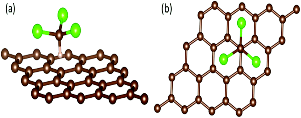Fig. 10 The most stable configuration for chloroform molecule adsorbed at graphene surface. The brown, green and pink atoms are corresponding to C, Cl, and H, respectively. (a) Side view. (b) Top view.

The band structure has been calculated with the distance between the chloroform molecule and the graphene surface in the region of 1.0–3.0 Å. It is well known that the pure graphene has high conductivity due to its zero band gap.⁴³ However, it is obvious in Fig. 11(a) that band gap was opened near the Fermi energy when chloroform molecule was adsorbed to the graphene, which means that the conductivity of the adsorption system was reduced compared with pure graphene. In addition, the value of the band gap reduced quickly with the increase of adsorption distance as shown in Fig. 11(b). Therefore, it can be concluded that the relative resistance of the graphene will increase with the chloroform molecule adsorbing on the graphene and decrease with desorption of chloroform molecule from the graphene. This conclusion was in consistent with the relative resistance curve in Fig. 5(b) including adsorption and desorption process. Different adsorbed molecules will induce different band structure of the graphene and subsequently result in diverse resistance curve shapes. This is the theoretical mechanism for GCSs to discriminate chemical molecules with broad selectivity by time-domain resistance curves.

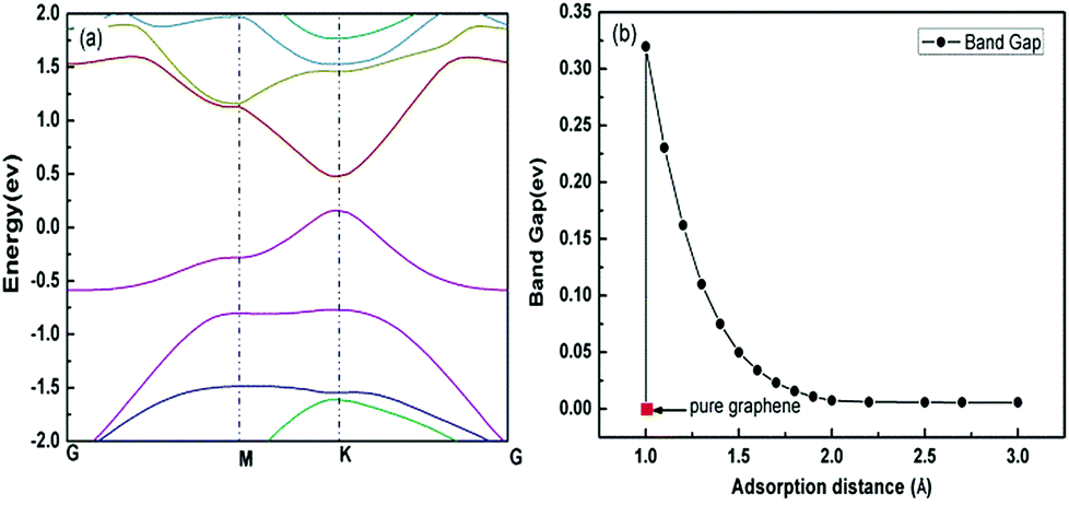Fig. 11 Band structure of graphene with adsorption of chloroform molecule. (a) Band structure of graphene with the adsorption distances 1 Å. (b) Relationship between the band gap and the adsorption distances.

4. Conclusions

According to different response curves of adsorption and desorption for chemical molecules on the interface of graphene, a chemical sensor based on unmodified 3D graphene foam was constructed to discriminate target molecules with broad selectivity through pattern recognition of time-domain resistance curves but not surface modifications. The results showed that the predictive accuracy could be above 98% for six kinds of chemical molecules which exhibited excellent broad selectivity. Compared with the existing work^6,25,26 which use two-dimensional graphene with a complex electrode and low frequency noise spectra, our chemical sensor was much easier for fabrication with high classification accuracy. Furthermore, based on the first principle, we found that the electrical characteristics could be changed by the distance between molecules and graphene surface, which have provided a possible theory explanation why pattern recognition could be used to make GCS be selectivity. This work may have presented a new strategy for design of graphene chemical sensors. The future researches of this work in our group include new algorithms for targets discrimination in mixture compounds and optimization of theoretical calculation, which both will undoubtedly be more meaningful for chemical sensor designation with graphene.

Conflicts of interest

There are no conflicts to declare.

Acknowledgements

This research project was jointly supported by the National Natural Science Foundation of China (Grant No. 61401258, 11674199, 11674197, 21303096 and 61401259), the China Postdoctoral Science Foundation (Grant No. 2013M541952) and the College Independent Innovation Plan of Jinan (Grant No. 201401236).

Notes and references

1. X. Li, J. Sha, S. K. Lee, Y. Li, Y. Ji, Y. Zhao and J. M. Tour, ACS Nano, 2016, 10, 7307–7313.
2. S. Morozov, K. Novoselov, M. Katsnelson, F. Schedin, D. Elias, J. Jaszczak and A. Geim, Phys. Rev. Lett., 2008, 100(1), 145–150.
3. M. H. Kang, L. O. PrietoLópez, B. Chen, K. Teo, J. A. Williams, W. I. Milne and M. T. Cole, ACS Appl. Mater. Interfaces, 2016, 8(34), 22506–22515.
4. K. S. Novoselov, A. K. Geim, S. V. Morozov, D. Jiang, Y. Zhang, S. V. Dubonos, I. V. Grigorieva and A. A. Firsov, Science, 2004, 306(5696), 666–669.
5. F. Yavari and N. Koratkar, J. Phys. Chem. Lett., 2012, 3, 1746–1753.
6. E. C. Nallon, V. P. Schnee, C. Bright, M. P. Polcha and Q. Li, ACS Sens., 2015, 1, 26–31.
7. R. K. Paul, S. Badhulika, N. M. Saucedo and A. Mulchandani, Anal. Chem., 2012, 84, 8171–8178.
8. S. J. Park, O. S. Kwon, S. H. Lee, H. S. Song, T. H. Park and J. Jang, Nano Lett., 2012, 12(10), 5082–5090.
9. B. Cai, S. Wang, L. Huang, Y. Ning, Z. Zhang and G. J. Zhang, ACS Nano, 2014, 8(3), 2632–2638.
10. N. Tammanoon, A. Wisitsoraat, C. Sriprachuabwong, D. Phokharatkul, A. Tuantranont, S. Phanichphant and C. Liewhiran, ACS Appl. Mater. Interfaces, 2015, 7(43), 24338–24352.
11. Y. V. Stebunov, O. A. Aftenieva, A. V. Arsenin and V. S. Volkov, ACS Appl. Mater. Interfaces, 2015, 7(39), 21727–21734.
12. X. Zhang, S. Xu, S. Jiang, J. Wang, J. Wei and S. Xu, Appl. Surf. Sci., 2015, 353, 63–70.
13. W. Yue, S. Jiang, S. Xu, Y. Ma and C. Bai, Sens. Actuators, B, 2015, 214, 204–210.
14. W. Yue, S. Jiang, S. Xu and C. Bai, Sens. Actuators, B, 2014, 195, 467–472.
15. S. Xu, S. Jiang, J. Wang, J. Wei, W. Yue and Y. Ma, Sens. Actuators, B, 2015, 222, 1175–1183.
16. X. Dong, Y. Shi, W. Huang, P. Chen and L. J. Li, Adv. Mater., 2010, 22, 1649–1653.
17. B. Jin, P. Wang, H. Mao, B. Hu, H. Zhang and Z. Cheng, Biosens. Bioelectron., 2013, 55, 464–469.
18. Y. H. Kwak, D. S. Choi, Y. N. Kim, H. Kim, D. H. Yoon and S. S. Ahn, Biosens. Bioelectron., 2012, 37, 82–87.
19. S. G. Chatterjee, S. Chatterjee, A. K. Ray and A. K. Chakraborty, Sens. Actuators, B, 2015, 221, 1170–1181.
20. Z. Xie, X. Zuo, G. P. Zhang, Z. L. Li and C. K. Wang, Chem. Phys. Lett., 2016, 657, 18–25.
21. I. Choudhuri, N. Patra, A. Mahata, R. Ahuja and B. Pathak, J. Phys. Chem. C, 2015, 119, 24827–24836.
22. H. Liu, Z. Chen, S. Dai and D. E. Jiang, J. Solid State Chem., 2015, 224, 2–6.
23. V. Dobrokhotov, A. Larin and D. Sowell, Sensors., 2013, 13, 9016–9028.
24. A. A. Balandin, S. Rumyantsev, G. Liu and M. S. Shur, Nano Lett., 2012, 12, 2294–2298.
25. S. Rumyantsev, G. Liu, M. S. Shur, R. A. Potyrailo and A. A. Balandin, Nano Lett., 2012, 12, 2294–2298.
26. C. Nallon Eric, P. Schnee Vincent and J. Bright Collin, Anal. Chem., 2016, 2, 1401–1406.
27. Y. Ma, M. Zhao, B. Cai, W. Wang, Z. Ye and J. Huang, Biosens. Bioelectron., 2014, 59, 384–388.
28. L. Wang, Y. Zhang, J. Yu, J. He, H. Yang and Y. Ye, Sens. Actuators, B, 2017, 239, 172–179.
29. K. R. Amin and A. Bid, ACS Appl. Mater. Interfaces, 2015, 7, 19825–19830.
30. C. Cortes and V. Vapnik, Mach. Learn., 1995, 20, 273–297.
31. D. Chen, Y. Tian and X. Liu, Pattern Recogn., 2016, 60, 296–305.
32. R. E. Fan, P. H. Chen and C. J. Lin, J. Mach. Learn. Res., 2005, 6, 1889–1918.
33. B. Schölkopf, A. Smola, R. Williamson and P. Bartlett, Neural Comput., 2000, 12, 1207–1245.
34. Z. Chen, W. Ren, L. Gao, B. Liu, S. Pei and H. M. Cheng, Nat. Mater., 2011, 10(6), 424–428.
35. P. Trinsoutrot, H. Vergnes and B. Caussat, Mater. Sci. Eng., B, 2014, 179, 12–16.
36. W. Jiang, H. Xin and W. Li, Mater. Lett., 2016, 162, 105–109.
37. C. C. Chang and C. J. Lin, ACM T. Intel. Syst. Tec., 2007, 2, 389–396.
38. A. Ambrosetti and P. L. Silvestrelli, Gas separation in nanoporous graphene from first principle calculations, J. Phys. Chem. C, 2014, 118(33), 19172–19179.
39. Y. Tao, Q. Xue, Z. Liu, M. Shan, C. Ling, T. Wu and X. Li, Tunable hydrogen separation in porous graphene membrane: first principle and molecular dynamic simulation, ACS Appl. Mater. Interfaces, 2014, 6(11), 8048–8058.
40. G. Kresse and J. Hafner, Ab Initio Molecular Dynamics for Liquid Metals, Phys. Rev. B: Condens. Matter Mater. Phys., 1993, 47, 558–561.
41. G. Kresse and J. Furthmüller, Efficient Iterative Schemes for Ab Initio Total Energy Calculations Using a Plane Wave Basis Set, Phys. Rev. B: Condens. Matter Mater. Phys., 1996, 54, 11169–11186.
42. J. P. Perdew, K. Burke and M. Ernzerhof, Generalized gradient approximation made simple, Phys. Rev. Lett., 1996, 77(18), 3865.
43. A. K. Geim and K. S. Novoselov, The rise of graphene, Nat. Mater., 2007, 6(3), 183–191.

---