DOI:
10.1039/C7RA07587A
(Paper)
RSC Adv., 2017,
7, 46378-46387
Solubility modelling, solution thermodynamics and preferential solvation of hymecromone in binary solvent mixtures of N,N-dimethylformamide + methanol, ethanol or n-propanol†
Received
10th July 2017
, Accepted 26th September 2017
First published on 2nd October 2017
Abstract
Solubilities of hymecromone in neat solvents of N,N-dimethylformamide (DMF), methanol, ethanol and n-propanol, and their binary mixed solvents of DMF + methanol, DMF + ethanol and DMF + n-propanol were determined using an isothermal dissolution equilibrium method within the temperature range from 278.15 K to 313.15 K under 101.1 kPa. They were correlated with the Jouyban–Acree, van't Hoff–Jouyban–Acree and Apelblat–Jouyban–Acree models obtaining relative average deviations (RAD) lower than 0.51% and root-mean-square deviation (RMSD) lower than 4.42 × 10⁻⁴. Positive values of the dissolution enthalpy illustrated that the dissolution process of hymecromone in these mixed solvents was endothermic. Furthermore, the preferential solvation parameters were derived by using the inverse Kirkwood–Buff integrals. The preferential solvation parameters (δx1,3) were negative in alcohol-rich mixtures but positive in compositions from 0.35 (0.43, 0.50) in the mole fraction of DMF to neat DMF.
Introduction
Solid–liquid equilibrium data thermodynamically important because it can provide necessary information for the design, analysis and optimization of separation and purification processes in various fields e.g. pharmaceutical, chemical, food, petrochemical and materials.1 The solubility behavior of drugs in solvent mixtures as a function of composition and temperature is evaluated essentially for the purposes of raw material purification, design of liquid dosage forms, and understanding of the mechanisms relating to the physical and chemical stability of pharmaceutical dissolutions.2,3
Hymecromone (CAS Registry no. 90-33-5, chemical structure shown in Fig. S1 of the ESI†), also named 4-methylumbelliferone, 7-hydroxy-4-methylcoumarin or 7-hydroxy-4-methyl-2H-benzo[b]-pyran-2-one, is used commercially for choleretic and antispasmodic drugs4–6 and as a standard for the fluorometric determination of enzyme activity,7,8 and it is also the starting material for the production of laser dyes9,10 and some insecticides.11,12 Due to its good properties, hymecromone has been received great attention. The synthesis of hymecromone have been reported in some literatures.11,12 However, the reaction product is crude hymecromone contaminated with 4,4′-dimethylcoumarin-7,6-α-pyrone. With the development of pharmaceutical and dye industry, the requirements for hymecromone purity are becoming higher. The impurity restricts its uses in many aspects. For example, as an important intermediate for laser dye, pure hymecromone is needed in making high purity laser dye, where impurities in the starting material might affect the dye properties of synthesized material. In order to extend the application of hymecromone, it is vital to isolate and purify the crude product.
In the previous works, the purification for hymecromone is by adding the crude hymecromone into an aqueous alkali metal hydroxide, and then acidifying the solid to yield pure hymecromone.9,13,14 However the cost of the process is very high. It is well-known that crystallization or recrystallization is commonly used as a purification step in its production process. This method has been applied in industrial production because of its low energy consumption, high purity, and simple production equipment. A basic step in purification and improve productivity of chemical substance is to determine its solubility behavior and thermodynamic properties of solutions, which can give a demonstrative description of its physicochemical properties, thermodynamic functions and the mechanisms relating to the physical and chemical stability of pharmaceutical dissolutions. In order to develop the new purification method via solvent crystallization, the solubility data of hymecromone in different solvents are of clear importance for the quality of the final product.1–3 Knowledge of the solubility enables to discover the appropriate solvent system for purifying hymecromone via crystallization. To the best of our knowledge, the solubility of hymecromone in solvents and solvent mixtures cannot be found in the open publications.
In this work, we determine the solubility of hymecromone in some organic solvents and solvent mixtures and develop better models for describing these behaviors. DMF is a very interesting co-solvent to study the interrelation between drug solubility and medium polarity.15,16 Methanol is not used to develop liquid medicines due to its high toxicity. But in some instances methanol is used in drug purification procedures,17 as well as solvent in some drug microencapsulation techniques.18 Moreover, methanol is widely used as mobile phase in high performance liquid chromatography.19 Ethanol is a common and safe co-solvent to be used in pharmaceutical liquid formulations. Its solubilization power is reasonably high and usually used in the liquid formulations at concentrations lower than 50%. In addition to solubility enhancement of ethanol, it can affect a drug's absorption, distribution, metabolism, and excretion.20 On the other hand, although n-propanol is not widely used as co-solvent for design of liquid medicines, it has been used as solvent in the pharmaceutical industry for resins and cellulose esters.21,22 Therefore, we choice four commonly used organic solvents, DMF, methanol, ethanol and n-propanol, and liquid mixtures of (DMF + methanol), (DMF + ethanol) and (DMF + n-propanol) in industrial purification and reaction process. Specifically, the temperature of solvent-assisted crystallization of hymecromone is almost in the temperature range from 273 K to 320 K. On the basis of the considerations mentioned above, in this work, we carry out the systematic studies on solubility of hymecromone in neat solvents and mixed solvents formed by DMF, methanol, ethanol and n-propanol at temperature range from (278.15 to 313.15) K, and correlation with different models. In the following, the inverse Kirkwood–Buff integrals (IKBI) approach23–25 is applied to evaluate the preferential solvation of hymecromone in the binary mixtures analyzed.
Experimental section
Materials and apparatus
Hymecromone was provided by Shangdong Shuojiao Chemical Co., Ltd, China with a mass fraction of 0.986. It was purified three times via recrystallization in ethanol. The final content of hymecromone employed for solubility measurement was 0.996 in mass fraction, which was confirmed using a high-performance liquid chromatography (HPLC, Agilent-1260). The four solvents (methanol, ethanol, n-propanol, and DMF) were of analytical grade, which were provided by Sinopharm Chemical Reagent Co., Ltd., China. The purity of these solvents was all higher than 0.993 in mass fractions, which were determined by gas chromatography {GC Smart (GC-2018)}. The detailed information of these chemicals used in this work was collected and presented in Table 1.
Table 1 Detailed information of hymecromone and the selected solvents
| Chemicals |
Molar mass g mol−1 |
Melting point K |
Melting enthalpy kJ mol−1 |
Density kg m−3 (295 K) |
Source |
Initial mass fraction purity |
Purification method |
Final mass fraction purity |
Analytical method |
| Take from ref. 44. Calculated using Advanced Chemistry Development (ACD/Labs) Software V11.02 (© 1994–2017 ACD/Labs). High-performance liquid chromatography. Gas chromatography. |
| Hymecromone |
176.17 |
460.7a |
29.14a |
1319b |
Shangdong Shuojia Chemical Co., Ltd, China |
0.986 |
Recrystallization |
0.996 |
HPLCc |
| Methanol |
32.04 |
|
|
|
Sinopharm Chemical Reagent Co., Ltd., China |
0.994 |
— |
0.994 |
GCd |
| Ethanol |
46.07 |
|
|
|
0.993 |
— |
0.993 |
GC |
| n-Propanol |
60.06 |
|
|
|
0.995 |
— |
0.995 |
GC |
| DMF |
73.09 |
|
|
|
0.995 |
— |
0.995 |
GC |
The experimental apparatus26,27 employed in the solubility determination included a 100 ml jacketed glass vessel with a magnetic stirrer and a circulating (water + isopropanol) system used for keeping the system temperature. The temperature of circulating (water + isopropanol) was controlled by a thermostatic bath (model: QYHX-1030) with a standard uncertainty of 0.05 K purchased from Shanghai Joyn Electronic Co., Ltd., China. The true temperature of solution was displayed by a mercury glass micro thermometer (standard uncertainty: 0.02 K) inserted in the inner chamber of the jacket glass vessel. A condenser was connected with the glass vessel to prevent the solvent from escaping. Before experiment, the reliability of experimental apparatus was verified by measuring the benzoic acid solubility in toluene.26,27 An analytical balance (model: BSA224S) having a standard uncertainty of 0.0001 g was provided by Satorius Scientific Instrument (Beijing), which was employed to determine the mass of the solute, solvent, and saturated solution.
Preparation of solvent mixtures
The solvent mixtures were prepared by using the analytical balance (model: BSA224S) in our experiment. The mixed solvent in the glass vessel was about 60 ml. The mass fractions of DMF in the binary solvent mixtures varied from 0 to 1. The glass vessel was covered with a stopper to prevent the solvent from escaping during the preparation process of solvent mixtures. During the experiment, the atmospheric pressure was about 101.1 kPa.
Solubility measurement
In this work the solubility of hymecromone in neat solvents and binary solvent mixtures of (DMF + methanol), (DMF + ethanol) and (DMF + n-propanol) were determined by an isothermal dissolution equilibrium method,26–31 and the high-performance liquid phase chromatograph (HPLC, Agilent-1260) was employed to determine the solubility of hymecromone in equilibrium liquid phase.32,33
For each experiment, saturated solutions of hymecromone were prepared in the jacketed glass vessel. An excess of hymecromone was introduced into the jacketed glass vessel filled with about 60 ml neat solvent or solvent mixtures. Continuous stirring was achieved by using a magnetic stirrer at a given temperature to mix the solution intensively. The temperature of the solutions was maintained at a desired value by circulating (water + isopropanol) mixture from the thermostatic water bath through the outer jacket. In order to obtain the equilibration time of the studied systems, about 0.5 ml liquid phase was withdrawn every two hours by using a 2 ml of preheated syringe equipped with a pore syringe filter (PTFE 0.2 μm), and then analyzed by the high-performance liquid phase chromatograph (Agilent-1260). Once the analysis results didn't vary, the system was believed to be in equilibrium. In order to ensure that sampling was performed at equilibrium conditions, two types of experiments were carried out, one starting from a supersaturated solution, in which the solid phase precipitated to reach equilibrium and the other starting from a non-saturated solution, in which solid dissolved to reach equilibrium. The results demonstrated that it took about 13 h to reach equilibrium for all the studied systems. When the mixture arrived at equilibrium, the stirrer was turned off to allow any undissolved solute to be precipitated. One hour later, the upper liquid phase was taken out using the 2 ml of preheated or precooled syringe connected with a filter (PTFE 0.2 μm), and transferred rapidly to a pre-weighed volumetric flask equipped with a rubber stopper. The volumetric flask filled with sample was weighed again with the analytical balance. Subsequently, the sample was diluted with methanol, and 1 μl of the solution was withdrawn for analysis by using the HPLC.
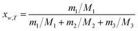
The equilibrium mole fraction solubility of hymecromone (xw,T) in neat solvents and the three binary solvent mixtures are obtained with eqn (1), and the initial compositions of binary solvent mixtures (w) are calculated with eqn (2) and (3).
| |
 | (1) |
| |
 | (2) |
| |
 | (3) |
here
m1 represents the mass of hymecromone,
m2 represents the mass of DMF, and
m3 represents the mass of methanol, ethanol, or
n-propanol, respectively.
M1,
M2 and
M3 are the corresponding molar mass.
Analysis method
The concentration of hymecromone was analyzed by the Agilent-1260 high-performance liquid chromatography (HPLC). The chromatographic column was a reverse phase column with a type of unimicro Kromasil C18, 5 μm (250 mm × 4.6 mm), which temperature was kept at 303 K. The wavelength of the UV detector was set to 322 nm.32,33 Pure methanol was used as mobile phase with the flow rate of 0.8 ml min−1. Each analysis was carried out three times, and the average value of three measurements was considered as the last value of the analysis. The relative standard uncertainty of the determination was estimated to be 0.026 in mole fraction.
X-ray powder diffraction
The samples hymecromone were analysed as collected without any further drying. They were identified by X-ray powder diffraction (XPRD) carried out on a HaoYuan DX-2700B (HaoYuan, China) instrument. The samples were determined by Cu Kα radiation (λ = 1.54184 nm), and the tube voltage and current were set at 40 kV and 30 mA, respectively. The data were collected at room temperature from 10° to 80° (2-theta) at a scan speed of 6 deg min−1 under atmospheric pressure.
Results and discussion
X-ray powder diffraction analysis
In order to demonstrate the existence of the polymorph transformation of hymecromone during the mutual solubility determination, the equilibrium solid phase is collected and analyzed by XRD. The patterns of the raw material and the solids crystallized in neat solvents and solvent mixtures are plotted in Fig. S2 of ESI.† It is confirmed by XRD pattern that all the XRD patterns of solid phase of hymecromone in equilibrium with its solution have the same characteristic peaks with the raw material. Whilst the presence of amorphous phases cannot be ruled out it can be concluded that there is possible no polymorph transformation during the entire experiment.
Solubility data
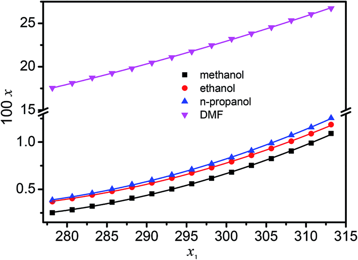
The determined mole fraction solubility (x) of hymecromone in methanol, ethanol, n-propanol and DMF within the temperature range from (278.15 to 313.15) K are presented in Tables S1–S3 of ESI,† and shown graphically in Fig. 1. It can be seen from the Fig. 1 that, for a certain neat solvent, the solubility of hymecromone increases with increasing temperature. At the fixed temperature, the mole fraction solubility of hymecromone is larger in DMF than in the alcohols. The mole fraction solubilities of hymecromone in different solvents decrease based the following order: DMF > n-propanol > ethanol > methanol. For example, at 298.15 K, the solubilities of hymecromone are 0.6170 × 10² in methanol, 0.7290 × 10² in ethanol, 0.7704 × 10² in n-propanol and 22.46 × 10² in DMF. However it is not possible to determine which solvent is suitable for the purification of hymecromone, because the solubility of the by-product 4,4′-dimethylcoumarin-7,6-α-pyrone is not known at present. This work is undertaken in our lab.
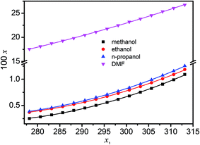 |
| | Fig. 1 Solubility (x) of hymecromone in mole fraction in neat organic solvents at different temperature: ■, methanol; ●, ethanol; ▲, n-propanol; ▼, DMF. The errors bars are smaller than the point size. | |
For the systems of hymecromone + alcohol, the mole fraction solubility is largest in n-propanol and lowest in methanol. The polarities of solvents seem to be a significant factor to affect the solubility of hymecromone in the selected alcohols. On the other hand, the DMF molecule has large dipole moments due to –NH– group, and may therefore give strong non-specific dipole–dipole interactions with hymecromone.34 It forms H-bonds with electron donor sites. These H-bonds with the solvent molecules have also a direct effect on the solubility. The solubilities of hymecromone are larger in DMF than in the other solvents. This case is obviously due to the formation of H-bonds between the N–H groups of DMF and (one of) the free electron pairs of the oxygen atoms in hymecromone molecules. Generally, it is too complicated to elucidate the solubility behavior presented in Tables S1–S3† based on a single reason. This behavior may be due to many factors, e.g., solute–solvent interactions, solvent–solvent interactions and molecular shapes and sizes and so on.
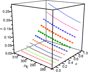
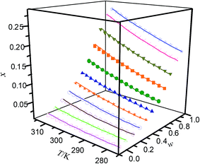
The determined mole fraction solubilities of hymecromone in binary solvent mixtures of (DMF + methanol), (DMF + ethanol) and (DMF + n-propanol) are also presented in Tables S1–S3 of ESI,† respectively. Furthermore, the relationship between the mole fraction solubility and temperature and solvent composition are shown graphically in Fig. 2–4. It can be seen from Tables S1–S3† that, for the studied solvent mixtures, the hymecromone solubility is a function of temperature and solvent composition. It increases with increasing temperature and mass fraction of DMF for the binary systems of (DMF + methanol), (DMF + ethanol) and (DMF + n-propanol), and the maximum solubility of hymecromone is observed in neat DMF.
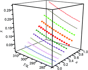 |
| | Fig. 2 Mole fraction solubility (x) of hymecromone in DMF (w) + methanol (1 − w) mixed solutions with various mass fractions at different temperatures: w, mass fraction of DMF; ☆, w = 1; ×, w = 0.8999; ▼, w = 0.7998; ■, w = 0.6969; ●, w = 0.5940; ▲, w = 0.4968; ★, w = 0.3995; ○, w = 0.2996; ◇, w = 0.1997; △, w = 0.0999; □, w = 0; —, calculated curves by the Jouyban–Acree model. The errors bars are smaller than the point size. | |
 |
| | Fig. 3 Mole fraction solubility (x) of hymecromone in DMF (w) + ethanol (1 − w) mixed solutions with various mass fractions at different temperatures: w, mass fraction of DMF; ☆, w = 1; ×, w = 0.9000; ▼, w = 0.8000; ■, w = 6998; ●, w = 0.5997; ▲, w = 0.4999; ★, w = 0.4002; ○, w = 3001; ◇, w = 0.1999; △, w = 0.0999; □, w = 0; —, calculated curves by the Jouyban–Acree model. The errors bars are smaller than the point size. | |
 |
| | Fig. 4 Mole fraction solubility (x) of hymecromone in DMF (w) + n-propanol (1 − w) mixed solutions with various mass fractions at different temperatures: w, mass fraction of DMF; ☆, w = 1; ×, w = 0.8995; ▼, w = 0.7990; ■, w = 6999; ●, w = 0.6008; ▲, w = 0.5001; ★, w = 0.3993; ○, w = 0.2995; ◇, w = 0.1997; △, w = 0.0999; □, w = 0; —, calculated curves by the Jouyban–Acree model. The errors bars are smaller than the point size. | |
Solubility modelling
Many models have been used to correlate the solubility of a solid in mixed solvent in previous publications. In this work, three models are employed to correlate the solubility of hymecromone in binary solvent mixtures of (DMF + methanol), (DMF + ethanol), and (DMF + n-propanol) at different temperatures, which correspond to Jouyban–Acree model,35 a combination of the Jouyban–Acree model with van't Hoff equation36,37 and a combination of the Jouyban–Acree model with modified Apelblat equation.36,37
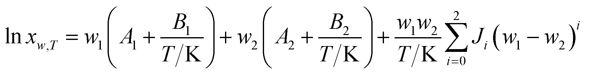
Jouyban–Acree model. The Jouyban–Acree model can offer accurate mathematical description for the dependence of solute solubility on both temperature and solvent composition for binary and ternary mixed solvents.35 It is expressed as eqn (4).| |
 | (4) |
where xw,T denotes the mole fraction solubility of solute in solvent mixtures at absolute temperature T in kelvin; w1 and w2 are the mass fraction of solvents 1 (DMF) and 2 (methanol, ethanol, and n-propanol) in the absence of the solute (hymecromone), respectively; x1,T and x2,T are the solute solubility in mole fraction in neat solvent; and Ji are the Jouyban–Acree model parameters.
van't Hoff–Jouyban–Acree model. The van't Hoff equation is an ideal model, which is described as| |
 | (5) |
Combining eqn (4) and (5), the van't Hoff–Jouyban–Acree model can be derived36,37 and expressed as eqn (6).
| |
 | (6) |
Modified Apelblat–Jouyban–Acree model. The modified Apelblat equation is a semi-empirical model having three parameters. It may be employed to describe a nonlinear relationship between solubility (ln![[thin space (1/6-em)]](https://www.rsc.org/images/entities/char_2009.gif) xT) in neat solvent and reciprocal of absolute temperature (1/T) and is described as
xT) in neat solvent and reciprocal of absolute temperature (1/T) and is described as| |
 | (7) |
where A, B, and C are equation parameters; and also xT is the mole fraction solubility of hymecromone in studied neat solvents at absolute temperature T.By substituting eqn (7) into (4), the modified Apelblat–Jouyban–Acree model can be obtained as eqn (8).36,37
| |
 | (8) |
The experimental solubility values of hymecromone in (DMF + methanol), (DMF + ethanol) and (DMF + n-propanol) mixtures are correlated and calculated with eqn (4), (6) and (8) with the method of non-linear regression. The objective function is described as
| |
 | (9) |
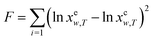
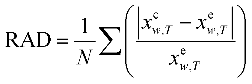
In order to show the error and evaluate the different models, the RAD and RMSD are also used, which are described as eqn (10) and (11).
| |
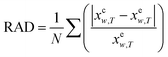 | (10) |
| |
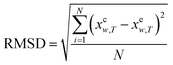 | (11) |
where
N is the number of experimental data points.
xew,T denotes the mole fraction solubility determined in this work; and
xcw,T, the mole fraction solubility calculated with corresponding solubility model.
Based on the experimental solubility data, the parameters in eqn (4), (6) and (8) are acquired by using nonlinear least-squares method with Mathcad software. The obtained values of model parameters are listed in Table S4 of ESI,† together with the RAD and the RMSD values. The solubilities of hymecromone in the three binary mixtures of (DMF + methanol), (DMF + ethanol), and (DMF + n-propanol) are evaluated based on the regressed parameters' values. The calculated solubilities by using the Jouyban–Acree model are plotted in Fig. 2–4. Table S4 of ESI† shows that for the selected binary solvent mixtures, the maximum value of relative average deviation (RAD) between the calculated and experimental values is 0.51%, which is obtained with the van't Hoff–Jouyban–Acree model for the system of (DMF + n-propanol). Besides, the RMSD values are no greater than 4.42 × 10⁻⁴. Comparison with the other three models, the values of RAD and RMSD obtained with the Jouyban–Acree model are relative small. On the whole, the three models can all be employed to correlate the solubility of hymecromone in the binary mixtures of (DMF + methanol), (DMF + ethanol) and (DMF + n-propanol) at all initial composition ranges.
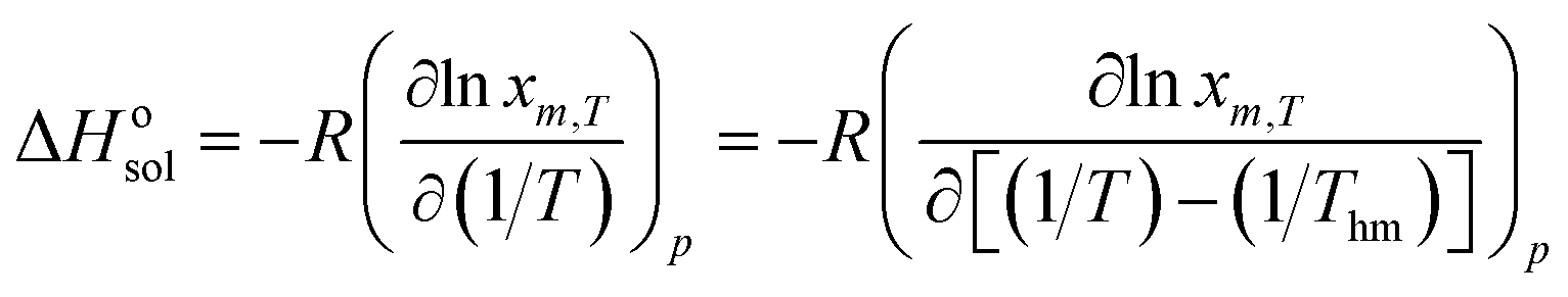
Dissolution properties for the dissolution
Thermodynamic properties of solute dissolved in solvent mixtures can provide important information regarding the dissolution process. The standard dissolution enthalpy (ΔHosol) for dissolution process of hymecromone in solvent mixtures can be obtained from the famous van't Hoff analysis.38| |
 | (12) |
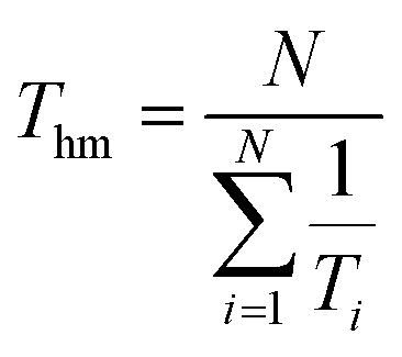
here R is the universal gas constant having a value of 8.314 J K−1 mol−1. Thm is the mean harmonic temperature which may be obtained via eqn (13).| |
 | (13) |
The values of ΔHosol be obtained from the slope of the curves of lnxm,T vs. (1/T−1/Thm). Fig. S3–S5 of ESI† present the curves of lnxm,T ∼ (1/T−1/Thm) for hymecromone dissolved in the binary mixed solvents of (DMF + methanol), (DMF + ethanol) and (DMF + n-propanol). The dissolution standard enthalpies of hymecromone in (DMF + methanol), (DMF + ethanol) and (DMF + n-propanol) are computed from eqn (12). The calculated values in the studied mixed solutions are tabulated in Table S5 of ESI.† It can be found from Table S5† that the values of standard molar enthalpy of dissolution are all positive, which show that the dissolution process of hymecromone in the three binary solvent solutions is endothermic, and the entropy is the driving force for the dissolution process.
Activity coefficients
The ideal solubility of solid hymecromone (xid) is calculated by using eqn (14).39,40| |
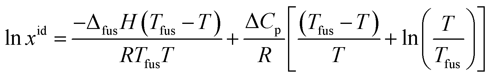
 | (14) |
where ΔfusH is the fusion enthalpy at fusion temperature Tfus. ΔCp is the difference between the molar heat capacity of the crystalline solid form and that of the hypothetical super-cooled liquid form. It has been generally assumed that ΔCp may be set approximately as the entropy of fusion (ΔfusS).40–42 The reasons for this hypothesis have already been discussed in the ref. 43.
The melting temperature, melting enthalpy and melting entropy for hymecromone can be found in ref. 44, which are 460.7 K, 29.14 kJ mol−1 and 63.42 J (K mol)−1, respectively. For the calculation of xidl values of solid hymecromone, all the parameters of eqn (14) are known now. Therefore, these values were calculated using eqn (14) and resulting values are presented in Tables S1–S3 of ESI.† The activity coefficients (γ3) of solid hymecromone in different neat solvents and solvent mixtures are calculated using eqn (15) from the respective ideal and experimental solubility data presented in Tables S1–S3 of ESI.†39–41
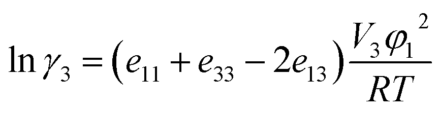
The calculated values of γ3 for solid hymecromone are presented in Tables S6–S8 of ESI.† These values are a measure of the deviation observed in real solution processes from the ideal solution processes. In alcohol-rich mixtures the γ3 values are slightly higher in DMF + methanol mixtures than in DMF + ethanol and DMF + n-propanol mixtures but a little different can be observed in DMF-rich mixtures. A rough estimate of solute–solvent intermolecular interactions can be made from γ3 values by considering the following expression:40,45
| |
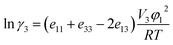 | (16) |
where subscript 1 stands for the solvent (in the present case, the DMF + methanol, DMF + ethanol or DMF +
n-propanol mixtures); and 3, solute hymecromone. Thus,
e11,
e33 and
e13 represent the solvent–solvent, solute–solute and solvent–solute interaction energies, respectively;
V3 is the molar volume of the supercooled liquid solute; and finally,
φ1 is the volume fraction of the solvent. The term
V3φ12/
RT may be considered almost constant in mixtures. In this way,
γ3 will depend mainly on
e11,
e33 and
e13.
40,45 The
e11 and
e33 terms are unfavorable for the drug solution processes, whereas the
e13 term favors these processes. Normally, the contribution of the
e33 term could be considered as constant in all the mixtures studied.
The following analysis can be made in a qualitative approach based on the energetic quantities and magnitudes described in the eqn (16). The term e11 is highest in neat alcohol and is smallest in DMF. Alcohol and alcohol-rich mixtures having larger γ3 values would imply high e11 and low e13 values. On the other hand, for the three solvent mixture in intermediate composition and DMF-rich mixtures or neat DMF (exhibiting a γ3 value <1), the e11 values are relatively low and the e13 values should be relatively high. Accordingly, the solvation of hymecromone should be higher in DMF-rich mixtures. In alcohol and alcohol-rich mixtures the γ3 values are dependent upon temperature, diminishing with increasing temperature.
Preferential solvation of hymecromone
The inverse Kirkwood–Buff integrals (IKBI) method is useful for evaluating the preferential solvation of nonelectrolyte in binary solvent mixtures, describing the local solvent composition around the solute in comparison with the global mixtures composition.23–25 This treatment depends on the values of the standard molar Gibbs energies of transfer of the solute from neat alcohol to the DMF (1) + alcohol (2) solvent mixtures and the excess molar Gibbs energy of mixing for the binary mixtures. As it has well been indicated in the literatures,23–25,46–49 preferential solvation studies provide valuable information regarding molecular interactions and the solvent distribution surrounding a solute molecule dissolved in solvent mixtures. It allows analyzing the local environment around the solute molecules describing the local fraction of the solvent components in the surrounding of the solute.
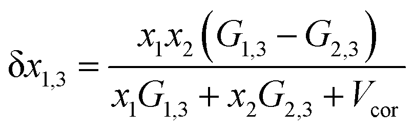
In binary co-solvent systems such as DMF (1) + methanol (2), DMF (1) + ethanol (2) and DMF (1) + n-propanol (2) mixtures, the preferential solvation parameter of hymecromone (compound 3) by the DMF (compound 1) is defined according to the following equation:23–25,46–49
| | |
δx1,3 = xL1,3 − x1 = −δx2,3
| (17) |
where
xL1,3 is the local mole fraction of the DMF in the environment near to the solute (solvation sphere) and
x1 is the mole fraction of the DMF used in the bulk solvent mixture. The δ
x1,3 parameter represents the excess or deficiency of MDF in the DMF mixture in the local region. When the solute is preferentially solvated by DMF (1), δ
x1,3 > 0; while δ
x1,3 is <0, the solute is said to be preferentially solvated by solvent (2). Nevertheless, when |δ
x1,3| < 0.01, the preferential solvation process is negligible, but if
xL1,3 ≈ 1, then complete solvation of the solute is performed by the DMF. The required parameter δ
x1,3 in DMF systems can be obtained from the inverse Kirkwood–Buff integrals (IKBI) for the individual solvent components analyzed according to some thermodynamic quantities as shown in the following equations:
23–25,46–49| |
 | (18) |
with,
| |
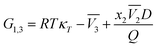 | (19) |
| |
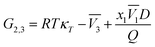 | (20) |
| |
 | (21) |
In these equations, κT is the isothermal compressibility of the DMF (1) + methanol (2), DMF (1) + ethanol (2) and DMF (1) + n-propanol (2) solvent mixtures (in GPa−1). The dependence of κT on composition is not known for a lot of the systems investigated. On the other hand, due to the small contribution of RTκT to the inverse Kirkwood–Buff integral, the dependence of κT on composition will be calculated approximated considering additive behavior from individual isothermal compressibilities of components according to the eqn (22).24,25,46–49
| | |
κT = x1κoT,1 + x2κoT,2
| (22) |
here
xi is the volume fraction of component
i in the mixture and
κoT,i is the isothermal compressibility of the neat solvent
i. The values of
RTκT in different binary DMF (1) + methanol (2), DMF (1) + ethanol (2) and DMF (1) +
n-propanol (2) mixtures are calculated using
eqn (22) with the
κoT,i values 0.653, 1.248, 1.153 and 1.025 GPa
−1 for DMF, methanol, ethanol and
n-propanol, respectively.
50
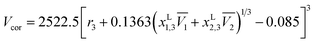
In eqn (19)–(21),  and
and  are the partial molar volumes of the solvents in the mixtures (in cm3 mol−1); similarly,
  is the partial molar volume of hymecromone in these mixtures. Because no partial molar volume of hymecromone (3) in these mixtures are reported in the literature, in this work this property is considered as similar to that for the pure compound as a good approximation49 with the value 133.5 cm3 mol−1, which is calculated on the basis of the molar mass and density of hymecromone calculated using Advanced Chemistry Development (ACD/Labs) Software V11.02 (© 1994–2017 ACD/Labs). Thus, the molecular radius of hymecromone in eqn (13) is calculated by means of eqn (23)
| |
 | (23) |
here
r3 is molecular radius of hymecromone, and
NAv is the Avogadro's number.
The partial molar volumes of both solvents in the mixtures can be calculated based on the eqn (24) and (25) from the reported density values of the DMF (1) + alcohol (2) mixtures at the studied temperatures under study by Yang for DMF + methanol and DMF + ethanol mixtures51 and by Páez for DMF + n-propanol mixtures.52
| |
 | (24) |
| |
 | (25) |
In these equations V is the molar volume of the mixtures calculated as V =(x1M1 + x2M2)/ρ. Here, M1 is 32.04 g mol−1 for methanol, 46.07 g mol−1 for ethanol, 60.10 g mol−1 for n-propanol and M2 is 73.1 g mol−1 for DMF.
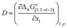
In eqn (19) and (20), the function D (eqn (26)) is the derivative of the standard molar Gibbs energies of transfer of solute from neat methanol, ethanol and n-propanol to DMF (1) + alcohol (2) mixtures with respect to the DMF composition (in kJ mol−1). The function Q (eqn (27)) involves the second derivative of the excess molar Gibbs energy of mixing of the two solvents (GExc1+2) with respect to the methanol, ethanol and n-propanol proportion in the mixtures (in kJ mol−1).23–25,46–49
| |
 | (26) |
| |
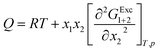 | (27) |
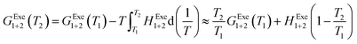
In order to calculate the Q values, the excess molar Gibbs energies of mixing GExc1+2 are needed. Nevertheless, these values are reported at not 298.15 K, but 313.15 K for DMF (1) + methanol (2) and DMF (1) + ethanol (2) mixtures,24 and 353.15 K for DMF (1) + n-propanol (2) mixtures.53 In this way, it is necessary to compute these values at the other temperatures required. GExc1+2 values (J mol−1) at 313.15 K are calculated according eqn (28) and (29) for the DMF (1) + methanol (2) and DMF (1) + ethanol (2) mixtures, respectively, as reported by Marcus.24 The GExc1+2 values (J mol−1) at 353.15 K are calculated in terms of the isothermal vapor + liquid equilibrium data for DMF (1) + n-propanol (2) mixtures,53 and regressed to a regular forth degree polynomial as a function of mole fraction of DMF, which are described as eqn (30). On the other hand, the GExc1+2 values at other temperatures are calculated using eqn (31), where HExc1+2 is the excess molar enthalpy of the DMF mixtures, T1 is 313.15 K for DMF (1) + methanol (2) and DMF (1) + ethanol (2) mixtures and 353.15 K for DMF (1) + n-propanol (2), and T2 is the temperature under consideration. HExc1+2 values for DMF (1) + methanol (2) and DMF (1) + ethanol (2) mixtures (expressed as eqn (32) and (33)) is taken from ref. 24; and for DMF (1) + n-propanol (2) mixtures, taken from ref. 54, and also regressed to a regular forth degree polynomial as a function of mole fraction of DMF expressed as eqn (34). The respective values are considered varying in 0.05 in mole fraction of DMF.
| | |
GExc1+2 = x1(1 − x1)[−1264 + 67(1 − 2x1)]
| (28) |
| | |
GExc1+2 = x1(1 − x1)[−506 + 85(1 − 2x1) + 34(1 − 2x1)2 + 27(1 − 2x1)3]
| (29) |
| | |
GExc1+2 = −0.0184 − 1.414 × 103x1 + 1.714 × 103x12 − 344.90x13 + 45.168x14
| (30) |
| |
 | (31) |
| | |
HExc1+2 = x1(1 − x1)[−428 + 47(1 − 2x1) − 126(1 − 2x1)2]
| (32) |
| | |
HExc1+2 = x1(1 − x1)[1612 − 447(1 − 2x1) − 292(1 − 2x1)2]
| (33) |
| | |
HExc1+2 = −0.624 + 2.412 × 103x1 − 1.176 × 103x12 − 16.683x13 − 1.219 × 103x14
| (34) |
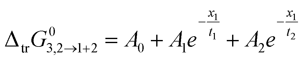
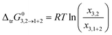
The standard molar Gibbs energy of transfer of hymecromone from neat methanol (2), ethanol (2) and n-propanol (2) to DMF (1) + methanol (2), DMF (1) + ethanol (2) and DMF (1) + n-propanol (2) mixtures is computed from the solubility data using eqn (35).
| |
 | (35) |
The values of ΔtrG03,2→1+2 are correlated with eqn (36) for DMF (1) + methanol (2) and DMF (1) + ethanol (2) mixtures, and with eqn (37) for DMF (1) + n-propanol (2) mixtures. Fig. S6 of ESI† shows the Gibbs energy of transfer behavior at different temperatures, whereas these values are presented in Tables S9 and S10 of ESI.† The obtained equation coefficients are tabulated in Table S11 of ESI.†
| |
 | (36) |
| | |
ΔtrG03,2→1+2 = a + bx1 + cx12 + dx13 + ex14 + fx15
| (37) |
Therefore, the values of D are obtained from the first derivative of eqn (36) and (37) solved according to the DMF mixture composition varying by 0.05 in mole fraction of DMF. The attained D values are presented in Tables S12 and S13 of ESI.† In addition, the calculated values of G1,3 and G2,3 are shown in Tables S14–S16 of ESI.† It can be seen that the G1,3 and G2,3 values are negative in all cases. This behavior indicates that hymecromone exhibits affinity for both solvents in the DMF (1) + methanol (2), DMF (1) + ethanol (2) and DMF (1) + n-propanol mixtures.
Definitive correlation volume depends on the local mole fractions around the solute, so it requires iteration. This iteration is done by replacing δx1,3 and Vcor in the eqn (17), (18) and (21) to recalculate xL1,3 until a non-variant value of Vcor is obtained. The acquired values of correlation volume Vcor and δx1,3 are presented in Tables S17–S19 of ESI† for DMF (1) + methanol (2), DMF (1) + ethanol (2) and DMF (1) + n-propanol (2) solvent mixtures, respectively. In addition, the dependence of δx1,3 values on DMF composition in mole fraction is shown graphically in Fig. 5. It demonstrates that the values of δx1,3 vary non-linearly with the DMF (1) proportion in all the solvent mixtures. According to Fig. 5, addition of DMF makes negative the δx1,3 values of hymecromone (3) from the neat methanol, ethanol and n-propanol to the mixture with composition x1 = 0.35 for DMF (1) + methanol (2), x1 = 0.43 for DMF (1) + ethanol (2) and x1 = 0.50 for DMF (1) + n-propanol (2) systems. Maximum negative values are attained in the mixture x1 = 0.05 with δx1,3 = −2.335 × 10⁻² to −2.621 × 10⁻² for DMF (1) + methanol (2), x1 = 0.15 with δx1,3 = −1.991 × 10⁻² to −2.312 × 10⁻² for DMF (1) + ethanol (2), and x1 = 0.15 with δx1,3 = −2.304 × 10⁻² to −2.705 × 10⁻² for DMF (1) + n-propanol (2), respectively. Probably the structuring of methanol, ethanol and n-propanol molecules around the nonpolar aromatic group of hymecromone contributes to lowering of the net δx1,3 to negative values in these methanol, ethanol or n-propanol-rich mixtures.
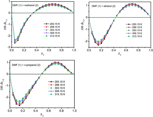 |
| | Fig. 5 δx1,3 values of hymecromone (3) from alcohol (2) to DMF (1) + methanol (2), DMF (1) + ethanol (2) and DMF (1) + n-propanol (2) mixtures at several temperatures. | |
In the DMF (1) + methanol (2) mixture with composition 0.35 < x1 < 1.00, DMF (1) + ethanol (2) mixture with composition 0.43 < x1 < 1.00, and DMF (1) + n-propanol (2) mixture with composition 0.50 < x1 < 1.00, the local mole fractions of DMF are higher than those of the mixtures and therefore the δx1,3 values are positive, which indicates that hymecromone is preferentially solvated by the DMF. The DMF action to increase the solute solubility may be associated to the breaking of the ordered structure of methanol, ethanol and n-propanol around the nonpolar moieties of hymecromone which increases the solvation of this solute exhibiting maximum value in x1 = 0.65 with δx1,3 = 0.648 × 10⁻² to 0.805 × 10⁻² for DMF (1) + methanol (2), x1 = 0.70 with δx1,3 = 0.992 × 10⁻² to 1.154 × 10⁻² for DMF (1) + ethanol (2), and x1 = 0.70 with δx1,3 = 0.869 × 10⁻² to 1.026 × 10⁻² for DMF (1) + n-propanol (2).
On the basis of a structural and functional group analysis, hymecromone can act as a Lewis acid in solution due to the ability of the acidic hydrogen atom in its –OH (Fig. S1 of ESI†) to establish hydrogen bonds with proton-acceptor functional groups of the solvents (oxygen atoms or nitrogen groups in DMF). In addition, hymecromone can act as a Lewis base because of the free electron pairs in oxygen atoms of ![[double bond, length as m-dash]](https://www.rsc.org/images/entities/char_e001.gif) O and –O– (Fig. S1 of ESI†), which interact with acidic hydrogen atoms of methanol, ethanol or n-propanol. Based on the preferential solvation results, it is conjecturable that in the regions (δx1,3 > 0) of 0.35 < x1 < 1.00 for DMF (1) + methanol (2) mixtures, 0.43 < x1 < 1.00 for DMF (1) + ethanol (2) mixtures, and 0.50 < x1 < 1.00 for DMF (1) + n-propanol (2) mixtures, hymecromone is acting as a Lewis acid with DMF molecules, even when this organic solvent is less basic than ethanol or n-propanol, as described by the Kamlet–Taft hydrogen bond acceptor parameters, i.e. β = 0.69 for DMF, β = 0.66 for methanol, β = 0.75 for ethanol, and 0.90 for n-propanol,50,55,56 respectively; while in the region of 0 < x1 < 0.35 for DMF (1) + methanol (2) mixtures, 0 < x1 < 0.43 for DMF (1) + ethanol (2) mixtures, and 0 < x1 < 0.50 for DMF (1) + n-propanol (2) mixtures, where hymecromone is preferentially solvated by methanol, ethanol or n-propanol, hymecromone is acting mainly as a Lewis base in front to methanol, ethanol or n-propanol because these solvents are more acidic than DMF molecules as described by the Kamlet–Taft hydrogen bond donor parameters, i.e. α = 0 for DMF, 0.990 for methanol, 0.850 for ethanol, and 0.766 for n-propanol, respectively.56,57
O and –O– (Fig. S1 of ESI†), which interact with acidic hydrogen atoms of methanol, ethanol or n-propanol. Based on the preferential solvation results, it is conjecturable that in the regions (δx1,3 > 0) of 0.35 < x1 < 1.00 for DMF (1) + methanol (2) mixtures, 0.43 < x1 < 1.00 for DMF (1) + ethanol (2) mixtures, and 0.50 < x1 < 1.00 for DMF (1) + n-propanol (2) mixtures, hymecromone is acting as a Lewis acid with DMF molecules, even when this organic solvent is less basic than ethanol or n-propanol, as described by the Kamlet–Taft hydrogen bond acceptor parameters, i.e. β = 0.69 for DMF, β = 0.66 for methanol, β = 0.75 for ethanol, and 0.90 for n-propanol,50,55,56 respectively; while in the region of 0 < x1 < 0.35 for DMF (1) + methanol (2) mixtures, 0 < x1 < 0.43 for DMF (1) + ethanol (2) mixtures, and 0 < x1 < 0.50 for DMF (1) + n-propanol (2) mixtures, where hymecromone is preferentially solvated by methanol, ethanol or n-propanol, hymecromone is acting mainly as a Lewis base in front to methanol, ethanol or n-propanol because these solvents are more acidic than DMF molecules as described by the Kamlet–Taft hydrogen bond donor parameters, i.e. α = 0 for DMF, 0.990 for methanol, 0.850 for ethanol, and 0.766 for n-propanol, respectively.56,57
Conclusion
The solubility of hymecromone in neat solvents of DMF, methanol, ethanol and n-propanol and three binary mixed solvents of (DMF + methanol), (DMF + ethanol) and (DMF + n-propanol) with various composition were acquired experimentally at temperature range from (278.15 to 313.15) K by using the isothermal dissolution equilibrium method under 101.1 kPa. For the three binary solvent mixtures, the mole fraction solubility of hymecromone increased with the increase in temperature and the mass fraction of DMF. The solubility data were correlated with the Jouyban–Acree model, van't Hoff–Jouyban–Acree model and Apelblat–Jouyban–Acree model. The values of RAD and RMSD were no greater than 0.51% and 4.42 × 10⁻⁴, respectively. The standard enthalpies for dissolution of hymecromone in the three mixed solvents were all positive, which showed that the dissolution process was endothermic. The solute–solvent intermolecular interactions were discussed in a qualitative approach. Quantitative values for the local mole fraction of methanol (ethanol or n-propanol) and DMF around the hymecromone were derived based on the IKBI method applied to the solubility data. Hymecromone was preferentially solvated by alcohol in alcohol-rich mixtures, and preferentially solvated by DMF in DMF-rich mixtures. At the same temperature, the preferential solvation magnitude of hymecromone by DMF was highest in ethanol mixtures, followed by n-propanol mixtures, and finally, by methanol mixtures. It is noteworthy that the solubility data presented in this work contribute to expansion of the physicochemical information about the solubility of drugs in binary solvent mixtures.
Conflicts of interest
There are no conflicts to declare.
Acknowledgements
This work was supported by the Science and Technology Research Key Project of the Education Department of Jiangsu Province (Project number: SJCX17_0621) and the Practice Innovation Project of Jiangsu Province for Post Graduate Students (Project number: XKYCX17_039). The authors would like to express their gratitude for the Priority Academic Program Development of Jiangsu Higher Education Institutions.
References
- J. Prausnitz and F. Tavares, AIChE J., 2004, 50, 739–761 CrossRef CAS.
- A. Jouyban, Handbook of solubility data for pharmaceuticals, CRC Press, BocaRaton, FL, 2010 Search PubMed.
- J. T. Rubino, Co-solvents and cosolvency, in Encyclopedia of pharmaceutical technology, 3, ed. J. Swarbrick and J. C. Boylan, Marcel Dekker, New York, NY, 1988 Search PubMed.
- H. Nakazawa, S. Yoshihara, D. Kudo, H. Morohashi, I. Kakizaki, K. Takagaki and M. Sasaki, Cancer Chemother. Pharmacol., 2006, 57, 165–170 CrossRef CAS PubMed.
- V. B. Lokeshwar, L. E. Lopez, D. Munoz, A. Chi, S. P. Shirodkar, S. D. Lokeshwar, D. O. Escudero, N. Dhir and N. Altman, Cancer Res., 2010, 70, 2613–2623 CrossRef CAS PubMed.
- A. Abate, V. Dimartino, P. Spina, P. L. Costa, C. Lombardo, A. Santini, M. del Piano and P. Alimonti, Drugs Exp. Clin. Res., 2001, 27, 223–231 CAS.
- K. Pritsch, S. Raidl, E. Marksteiner, H. Blaschke, R. Agerer, M. Schloter and A. Hartmann, J. Microbiol. Methods, 2004, 58, 233–241 CrossRef CAS PubMed.
- H. Zhi, J. Wang, S. Wang and Y. Wei, J. Spectrosc., 2013, 2013, 177–202 Search PubMed.
- S. Z. Zhang, CN Patent 101,712,811, May 26 2010.
- M. S. A. Abdel-Mottaleb, B. A. El-Sayed, M. M. Abo-Aly and M. Y. El-Kady, J. Photochem. Photobiol., A, 1989, 46, 379–390 CrossRef CAS.
- K. M. Khan, Z. S. Saify, S. Hayat, M. Z. Khan, F. Noor, T. Makhmoor, M. I. Choudhary, Zia-Ullah and S. Perveen, J. Chem. Soc. Pak., 2002, 24, 226–231 CAS.
- C. Gutiérrez-Sánchez, V. Calvino-Casilda, E. Pérez-Mayoral, R. M. Martín-Aranda, A. J. López-Peinado, M. Bejblová and J. čejka, Catal. Lett., 2009, 128, 318–322 CrossRef.
- S. Chachula, M. Fiks, R. Harasym and M. Trebacz, PL Patent 161,691, July 30 1993.
- H. Jozwiak, S. Kotlicki, W. Pietrzak and P. Guzicki, PL Patent 129,772, June 30 1984.
- A. J. Spiegel and M. M. Noseworthy, J. Pharm. Sci., 1963, 52, 917–927 CrossRef CAS PubMed.
- P. B. Rathi and V. K. Mourya, Indian J. Pharm. Sci., 2012, 74, 254–258 CrossRef CAS PubMed.
- B. Chen, Y. Du and H. Wang, Electrophoresis, 2010, 31, 371–377 CrossRef CAS PubMed.
- A. J. Thote and R. B. Gupta, Nanomedicine, 2005, 1, 85–90 CrossRef CAS PubMed.
- Y. Kazakevich and R. Lobrutto, HPLC for pharmaceutical scientists, John Wiley &Sons, Inc., Hoboken, NJ, 2007 Search PubMed.
- A. Jouyban, J. Shokri, M. Barzegar-Jalali, D. Hassanzadeh, W. E. Acree Jr, T. Ghafourian and A. Nokhodchi, J. Chem. Eng. Data, 2009, 54, 2142–2145 CrossRef CAS.
- S. H. Yalkowsky and Y. He, Handbook of aqueous solubility data, CRC Press, Boca Raton, 2003 Search PubMed.
- D. R. Delgado and F. Martínez, J. Solution Chem., 2014, 43, 836–852 CrossRef CAS.
- Y. Marcus, Preferential solvation in mixed solvents, in Fluctuation theory of solutions: Applications in
chemistry, chemical engineering, and biophysics, P. E. Smith, E. Matteoli and J. P. O'Connell, CRC Press, Boca Raton (FL), 2013 Search PubMed.
- Y. Marcus, Solvent mixtures: properties and selective solvation, Marcel Dekker, Inc., New York, 2002 Search PubMed.
- Y. Marcus, Pharm. Anal. Acta, 2017 DOI:10.4172/2153-2435.1000537.
- S. Han, L. Meng, C. B. Du, J. Xu, C. Cheng, J. Wang and H. K. Zhao, J. Chem. Eng. Data, 2016, 61, 2525–2535 CrossRef CAS.
- C. Cheng, Y. Cong, C. B. Du, J. Wang, G. B. Yao and H. K. Zhao, J. Chem. Thermodyn., 2016, 101, 372–379 CrossRef CAS.
- J. Wang, R. J. Xu and A. L. Xu, J. Chem. Thermodyn., 2017, 106, 132–144 CrossRef CAS.
- A. L. Xu, R. J. Xu and J. Wang, J. Chem. Thermodyn., 2016, 102, 188–198 CrossRef CAS.
- J. Wang, A. L. Xu and R. J. Xu, J. Chem. Thermodyn., 2017, 108, 45–58 CrossRef CAS.
- G. B. Yao, Z. X. Xia and Z. H. Li, J. Chem. Thermodyn., 2017, 105, 187–197 CrossRef CAS.
- L. Zhang and J. Zhu, Tradit. Chin. Drug Res. Clin. Pharmacol., 2006, 17, 222–224 CAS.
- M. Nakatama, M. Hiraoka, A. Matsuo, S. Hayashi and S. Ganno, Nippon Kagaku Kaishi, 1975, 96–99 CrossRef CAS.
- F. Huyskens, H. Morissen and P. Huyskens, J. Mol. Struct., 1998, 441, 17–25 CrossRef CAS.
- S. H. Eghrary, R. Zarghami, F. Martinez and A. Jouyban, J. Chem. Eng. Data, 2012, 57, 1544–1550 CrossRef CAS.
- A. Jouyban, M. A. A. Fakhree and W. E. Acree Jr, J. Chem. Eng. Data, 2012, 57, 1344–1346 CrossRef CAS.
- S. Vahdati, A. Shayanfar, J. Hanaee, F. Martínez, W. E. Acree Jr and A. Jouyban, Ind. Eng. Chem. Res., 2013, 52, 16630–16636 CrossRef CAS.
- N. J. Adel, M. Chokri and A. Arbi, J. Chem. Thermodyn., 2012, 55, 75–78 CrossRef.
- M. A. Ruidiaz, D. R. Delgado, F. Martínez and Y. Marcus, Fluid Phase Equilib., 2010, 299, 259–265 CrossRef CAS.
- F. Shakeel, S. Alshehri, M. A. Ibrahim, E. M. Elzayat, M. A. Altamimi, K. Mohsin, F. K. Alanazi and I. A. Alsarra, J. Mol. Liq., 2017, 234, 73–80 CrossRef CAS.
- Y. J. Manrique, D. P. Pacheco and F. Martínez, J. Solution Chem., 2008, 37, 165–181 CrossRef CAS.
- D. M. Aragón, A. Sosnik and F. Martínez, J. Solution Chem., 2009, 38, 1493–1503 CrossRef.
- S. H. Neau and G. L. Flynn, Pharm. Res., 1990, 7, 1157–1162 CrossRef CAS.
- X. Zhang, W. Huang, F. Tan, G. Xu and Z. Wu, Chin. Sci. Bull., 1989, 34, 1844–1845 CAS.
- A. Kristl and G. Vesnaver, J. Chem. Soc., Faraday Trans., 1995, 91, 995–998 RSC.
- Z. J. Cárdenas, D. M. Jiménez, D. R. Delgado, O. A. Almanza, A. Jouyban, F. Martínez and W. E. Acree Jr, J. Chem. Thermodyn., 2017, 108, 26–37 CrossRef.
- M. Jabbari, N. Khosravi, M. Feizabadi and D. Ajloo, RSC Adv., 2017, 7, 14776–14789 RSC.
- H. F. Tooski, M. Jabbari and A. Farajtabar, J. Solution Chem., 2016, 45, 1701–1714 CrossRef CAS.
- A. Jouyban, W. E. Acree Jr and F. Martínez, J. Mol. Liq., 2016, 224, 502–506 CrossRef CAS.
- Y. Marcus, The properties of solvents, John Wiley & Sons, Chichester, 1998 Search PubMed.
- C. S. Yang, Y. Sun, Y. F. He and P. S. Ma, J. Chem. Eng. Data, 2008, 53, 293–297 CrossRef CAS.
- M. S. Páez, M. K. Vergara and P. D. Cantero, Rev. Colomb. Quim., 2012, 41, 75–88 Search PubMed.
- C. M. Wang, H. R. Li, L. H. Zhu and S. J. Han, Fluid Phase Equilib., 2001, 189, 119–127 CrossRef CAS.
- H. Iloukhani and H. A. Zarei, J. Chem. Eng. Data, 2002, 47, 195–197 CrossRef CAS.
- M. J. Kamlet and R. W. Taft, J. Am. Chem. Soc., 1976, 98, 377–383 CrossRef CAS.
- A. Duereh, Y. Sato, R. L. Smith and H. Inomata, ACS Sustainable Chem. Eng., 2015, 3, 1881–1889 CrossRef CAS.
- R. W. Taft and M. J. Kamlet, J. Am. Chem. Soc., 1976, 98, 2886–2894 CrossRef CAS.
Footnote |
| † Electronic supplementary information (ESI) available. See DOI: 10.1039/c7ra07587a |
|
| This journal is © The Royal Society of Chemistry 2017 |
Click here to see how this site uses Cookies. View our privacy policy here. 
 Open Access Article
 This Open Access Article is licensed under a
  *b
*b


 and
and  are the partial molar volumes of the solvents in the mixtures (in cm3 mol−1); similarly,
  is the partial molar volume of hymecromone in these mixtures. Because no partial molar volume of hymecromone (3) in these mixtures are reported in the literature, in this work this property is considered as similar to that for the pure compound as a good approximation49 with the value 133.5 cm3 mol−1, which is calculated on the basis of the molar mass and density of hymecromone calculated using Advanced Chemistry Development (ACD/Labs) Software V11.02 (© 1994–2017 ACD/Labs). Thus, the molecular radius of hymecromone in eqn (13) is calculated by means of eqn (23)