
 Open Access Article
 This Open Access Article is licensed under a Creative Commons Attribution-Non Commercial 3.0 Unported Licence
Estimating contaminant source in chemical industry park using UAV-based monitoring platform, artificial neural network and atmospheric dispersion simulation
Sihang Qiu a,
Bin Chen*a,
Rongxiao Wanga,
Zhengqiu Zhua,
Yuan Wangb and
Xiaogang Qiua
a,
Bin Chen*a,
Rongxiao Wanga,
Zhengqiu Zhua,
Yuan Wangb and
Xiaogang Qiua
aCollege of Information System and Management, National University of Defense Technology, Changsha 410073, China. E-mail: nudtcb9372@gmail.com
bCollege of Territorial Resources and Tourism, Anhui Normal University, Wuhu 241003, China
First published on 15th August 2017
Abstract
Airborne contaminants emitted from chemical industry parks can pose a potential threat to the environment. Therefore, using the data obtained from concentration-monitoring of the contaminant to find the source is of high importance. Most previous source estimation methods collect meteorological parameters and concentration measurements from static sensors. However, some meteorological parameters such as atmospheric stability and cloud cover are difficult to measure precisely. Furthermore, installing only several static sensors does not provide enough sampling data. In this paper, a novel approach is proposed to find the location of an emission source as well as its release rate in a chemical industry park. An unmanned aerial vehicle (UAV) monitoring platform is applied to sample sufficient and high-quality concentration data. Afterwards, an artificial neural network (ANN) trained by an atmospheric dispersion simulation tool is used to locate and quantify the emission source from candidate solutions, bypassing data on the atmospheric stability and other hard-to-obtain meteorological parameters. A numerical simulation with different conditions is implemented to test the accuracy and stability of the proposed approach. A real experiment is conducted in Shanghai to test the performance and sensitivity of this approach as well as the robustness of the monitoring platform. The results show that the approach proposed in this paper can effectively estimate the contaminant source in chemical industry parks. Both the numerical and real experiments prove that the proposed method is less sensitive to errors in meteorological data and concentration measurements than traditional source estimation methods including Bayesian inference and optimization.
1 Introduction
With industrial development, airborne contaminants have seriously influenced the health of human beings. Monitoring industrial emissions has therefore become an important issue. Locating and quantifying contaminant sources is one of the essential tasks of air contaminant monitoring and chemical industry administration.1–5 Generally, in order to support accurate source estimation, a large number of monitoring stations should be established to sample sufficient high-quality monitoring data.6 Doubtlessly, building too many monitoring stations can be prohibitively expensive, and it is also difficult to manage a large number of stations. To address this challenge, we have developed an approach based on an unmanned aerial vehicle (UAV) monitoring platform, an artificial neural network (ANN) and an atmospheric dispersion simulation tool to find the optimal (most likely) atmospheric dispersion source.Generally, measurements of contaminants are obtained by static monitoring stations. However, static monitoring stations are usually not densely distributed enough to sample high-quality data containing useful information from the contaminant plume. In this case, it is difficult to estimate the emission source from the data collected from these monitoring stations even when they are equipped with high resolution sensors. As a result, researchers have attempted to use aircraft to obtain high-quality air concentration measurements of contaminants.6–14 For example, an aircraft was used for monitoring nitrogen emissions from point sources.9 A previous study also demonstrated a method of source estimation using remote aircraft.8 In addition, White et al. proposed a monitoring network based on UAV sensors.12,13 Sanada and Torii analyzed the radioactive pollutant concentration via an unmanned helicopter after the Fukushima Dai-ichi nuclear power plant accident.11 UAV platforms can also be applied for predicting the PM2.5 concentration,14 contaminant plumes and volcanic plumes.7,10 The use of UAV platforms therefore allows many problems in traditional monitoring methods using static sensors to be addressed.
An important application of concentration measurements is using them to locate and quantify the dispersion source of contaminants. In the past few years, many methods and tools have been used to find contaminant sources.15 Most estimation methods are based on Bayesian inference or optimization.6 With Bayesian inference, the dispersion source can be estimated by calculating the posterior function. The Markov Chain Monte Carlo (MCMC) algorithm is a useful tool for posterior function calculation and source estimation.3,8,16–18 Some advanced filter or optimization methods such as particle filter,19–21 EnKF,22 and PSO23,24 are also widely used in source estimation problems of chemical or nuclear power plants. However, the accuracies of traditional methods including Bayesian inference and optimization largely depend on the error of the model input and the accuracy of the forward dispersion modelling that is used in backward calculation. Furthermore, some input parameters such as atmospheric stability are quite difficult to measure and quantify. Therefore, methods such as using pre-determined scenarios for decision-making and bypassing the hard-to-obtain parameters have been proposed by researchers.25–28 These methods are able to estimate the source using neural networks or support vector machines without input data of certain complex parameters because a large number of pre-determined scenarios have already been applied for training and fitting. For example, a previous study estimated the release rate of a dispersion source via an ANN and optical sensor.28 Wang et al. bypassed the source term and used the integration of an ANN, gas detectors and PHAST to predict gas dispersion.27 The high accuracy of that study demonstrates that ANNs could be a useful tool for pollution forecasting and risk analysis. Moreover, an ANN was also applied for forecasting PM2.5 pollution and atmospheric dispersion of biological matter.29,30 Although ANNs have been extensively used in dispersion prediction, few researchers have applied an ANN in source location or quantification.
In this paper, a new approach is presented that is able to find the optimal emission source from candidate solutions using the measured data from a UAV. In order to generate high-quality training data for the ANN, an atmospheric dispersion simulation tool is used because the training input data are impossible to control in a real chemical industry park. The simulation tool uses the ANN to correct the traditional Gaussian diffusion model. The approach is then verified by numerical and real experiments. This approach can address the difficulties caused by the use of complex meteorological parameters as inputs. It is extremely insensible to measurement noise. Furthermore, the features of the ANN also make this novel approach more accurate than traditional methods. The experimental results show that the proposed source estimation method based on an ANN and a UAV is a useful and appropriate option for the management of a chemical industry park.
2 Methods
2.1 Remote monitoring system based on UAV platform
Conventional source estimation methods usually use concentration data from static monitoring stations. Therefore, the accuracy of the estimation results largely depends on the distribution and the number of monitoring stations. Generally, the more extensively and densely the monitoring stations are distributed, the more possible it is to identify the source correctly. Insufficient monitoring stations may cause large errors, especially when the contaminant plume does not pass directly over enough sensors. Measurements sampled near the central axis of the plume are more important because they provide more information on the features of the plume. We denote the measurements taken near the central axis “dominant data”. This study uses a remote monitoring system based on a UAV platform to obtain the dominant data together with the corresponding location information with the aim of overcoming the disadvantages of static monitoring stations. This monitoring system is highly mobile, which significantly increases the probability of successfully finding the emission source.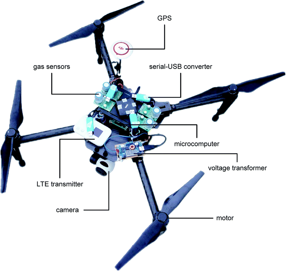 | ||
| Fig. 1 Air concentration monitoring system based on UAV platform. | ||
Furthermore, planning a flight route is a complex task because many conditions, such as the capacity of the battery, potential barriers to movement, electromagnetic interference and the weather, must be considered. A well designed flight route can greatly improve the accuracy of source estimation. In this paper, we will not discuss the flight route planning in detail since the focus is the method of locating and quantifying the contaminant source.
2.2 Source estimation using ANN
Artificial neural networks can be used for fitting or classifying complex non-linear systems. Conventional source estimation methods are mostly based on Bayesian theory or optimization. They estimate the source term via calculating the posterior probability distribution or optimizing a cost function. These two methods are useful when no candidate solutions are available. However, in industry parks, it is already known which emission points are the possible sources of contaminants. Therefore, we can restrict the search for the real source to these potential emission points (candidate solutions), which means that the source location problem can be regarded as a classification problem. Highly accurate results can be obtained if the structure of the ANN is well designed.In terms of traditional methods including Bayesian inference and optimization, it is clear that the inaccuracy in their results is mainly brought about by the errors in the input parameters. Clearly, some input parameters are impossible to directly measure using sensors. Therefore, to bypass these parameters, we use an atmospheric dispersion simulation tool to generate a sufficient number of pre-determined scenarios to cover all possible situations, and then use these scenarios to train the ANN. In Section 4, the experimental results show that the source estimation method based on the ANN is quite insensitive to these parameters.
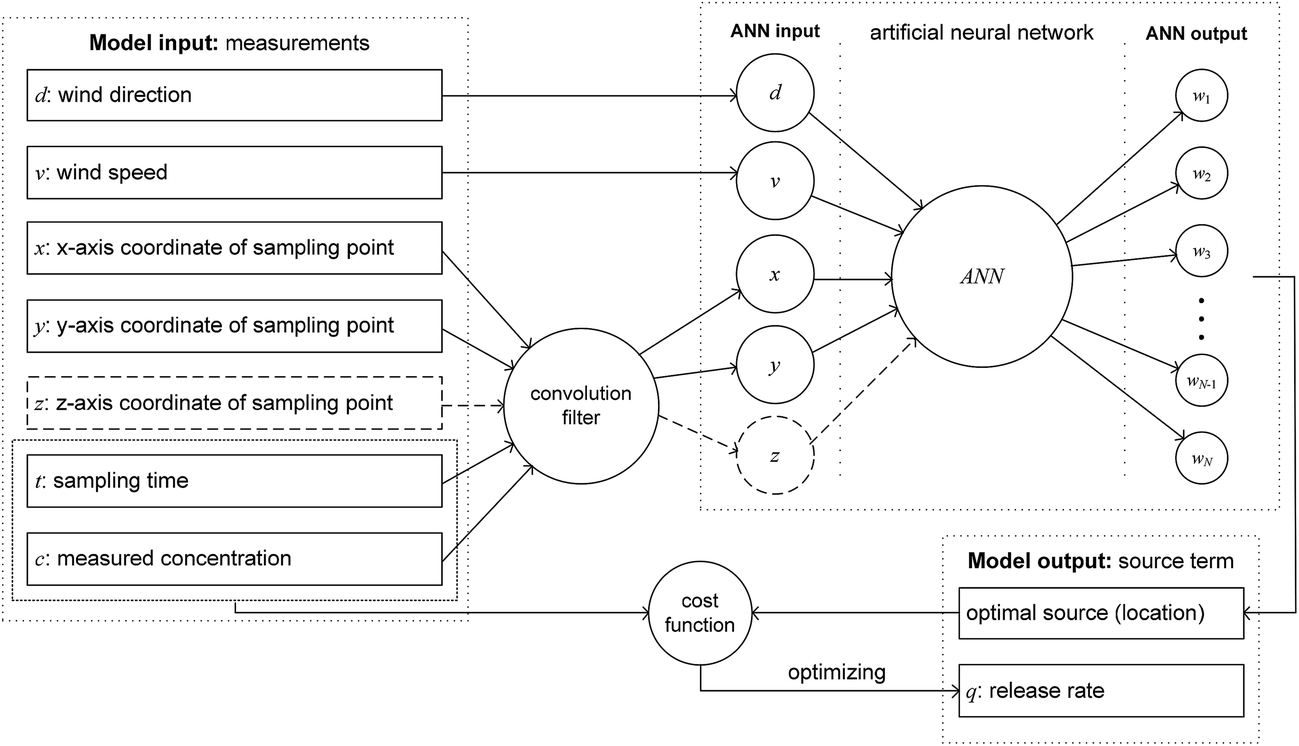 | ||
| Fig. 2 Mechanism of source estimation model. | ||
The ANN used in this study is a typical neural network with a single hidden layer. The number of neurons in the hidden layer depends on the number of candidate sources. In terms of the input and output of the ANN, the input includes: (1) a three-dimensional set {x,y,z} whose elements are the x-axis coordinate x, y-axis coordinate y, z-axis coordinate z of the sampling location of the dominant data; (2) wind speed v; and (3) wind direction d. In order to ensure the high quality of the sampling data and simplify the model, the aircraft usually moves at a constant height. In this case, we do not need to consider the parameter z. As for the output of the ANN, we denote the number of candidate sources {θi = (xi,yi,zi)}Ni=1 as N. Therefore, the output is an N-dimensional set output = {wi}Ni=1 that represents the weight of all candidates. The ith element wi represents the weight of the candidate source θi. A higher weight wi represents that the corresponding candidate θi is more likely to be the real emission source. If the real emission source is θp and the input is {x,y,z,d,v}, the expression of the output is shown as follows:
| Output = {wi|wi = δ[i − p]log10[f(θ,x,y,z,d,v) + 1],i ∈ Z,1 ≤ i ≤ N}, | (1) |
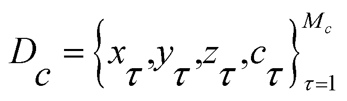 , where Mc means the number of elements in Dc.
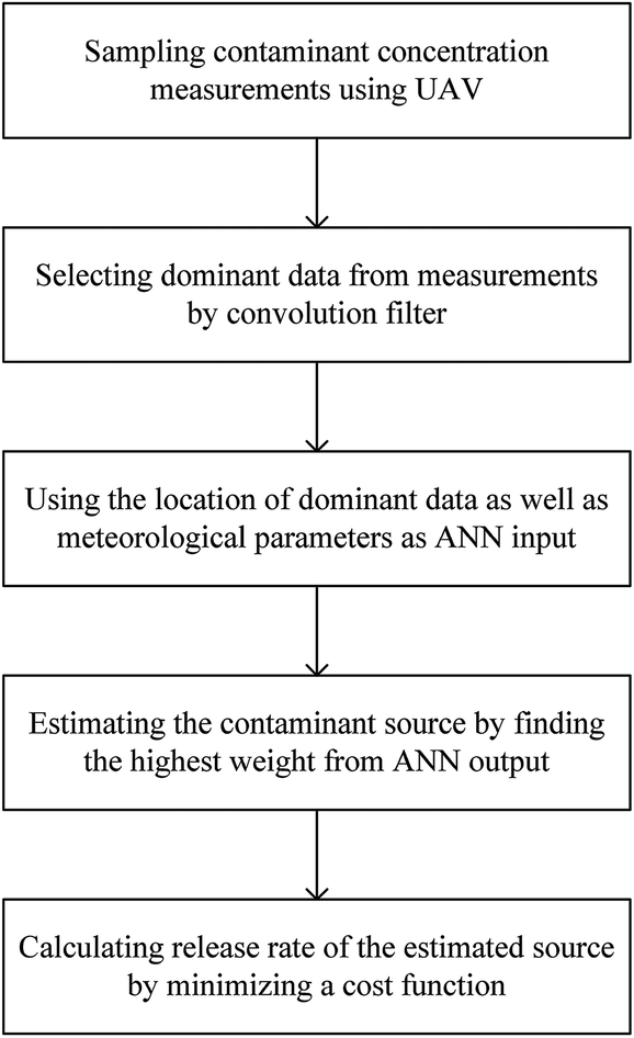 | ||
| Fig. 3 Process of source estimation. | ||
As a result, in the source estimation process, the input of the ANN is 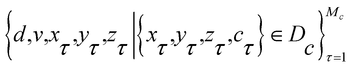 . Therefore, the output of the ANN is
 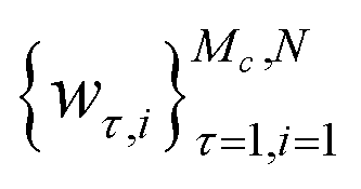 , where wτ,i means the weight of candidate source θi if the ANN input is {d,v,xτ,yτ,zτ}. However, each element in the input set may imply a different contaminant source. In order to address this problem, all the elements in the ANN output set are summed via the following equation:
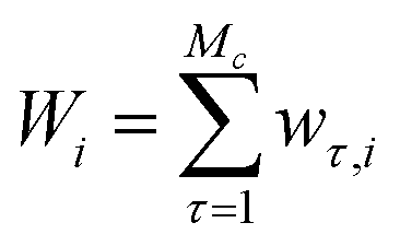 | (2) |
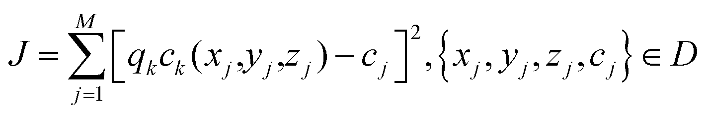 | (3) |
This cost function can be solved by various methods such as the least squares algorithm and gradient descent. By solving it, the complete source term including location and release rate is successfully obtained.
2.3 Contaminant atmospheric dispersion simulation and ANN training
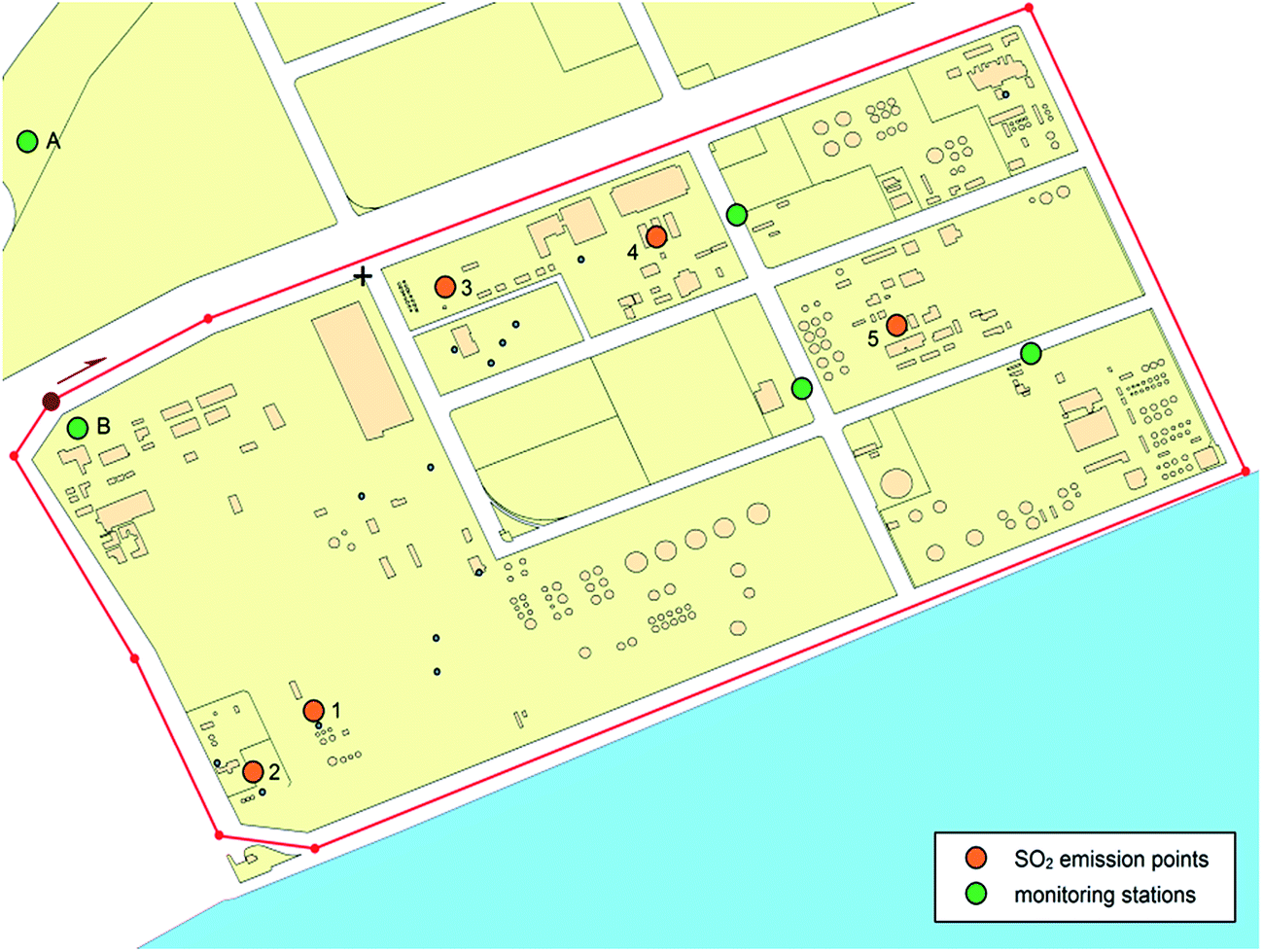 | ||
| Fig. 4 Map of experimental area. | ||
| No. | X | Y | Height | Explanation | Contaminants |
|---|---|---|---|---|---|
| 1 | −132.575 | −1317.63 | 50 | Waste incinerator for acrylonitrile (AN) | SO2, NOx, VOC, NH3 |
| 2 | −302.901 | −1483.42 | 68 | Chimney of sulfuric acid recovery (SAR) system | SO2, NOx, vitriol fog |
| 3 | 267.1415 | 0.359916 | 27 | Furnace no. 1 | SO2, PM2.5/PM10 |
| 4 | 861.3643 | 147.0462 | 27 | Furnace no. 2 | SO2, PM2.5/PM10 |
| 5 | 1532.017 | −142.542 | 30 | Hazardous waste incinerator | CO, SO2, NOx, PM2.5/PM10, HF, HCl, dioxin |
To simulate a contaminant dispersion scenario, several factors must be considered: emission source θi, meteorological parameters (wind direction d and wind speed v) and environmental conditions (atmospheric stability and terrain type over which the gas diffuses).
KD-ADSS is applied to model atmospheric dispersion.24 KD-ADSS is an atmospheric dispersion simulation tool based on neural networks and a Gaussian diffusion model. It uses neural networks to calibrate the accuracy of the traditional Gaussian model. From the input parameters shown in Table 2 it generates an output, which is the concentration value at the point of interest. This simulation tool has also been validated by the commercial software PHAST, the Indianapolis field study and a study of the Fukushima Dai-ichi nuclear accident. Thus, the concentration at sampling point (x,y,z) can be calculated by this simulation tool. The calculation of concentration data at each sampling point in the simulation can be illustrated by the function f(θ,x,y,z,d,v).
| Input symbol | Meaning |
|---|---|
| q | Release rate of emission source |
| W | Wind field. KD-ADSS also contains a wind field generation tool. |
| H | Height of emission source |
| Dx | Downwind distance of the interest point |
| Dy | Crosswind distance of the interest point |
| z | Height of the interest point |
| σy | Gaussian diffusion coefficient of y-axis |
| σz | Gaussian diffusion coefficient of z-axis |
| vs | Deposition/rise velocity |
| Other parameters concerning radionuclide | This case does not need these parameters |
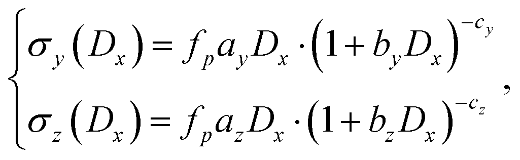
For the Gaussian diffusion coefficients σy and σz, their expressions are:33
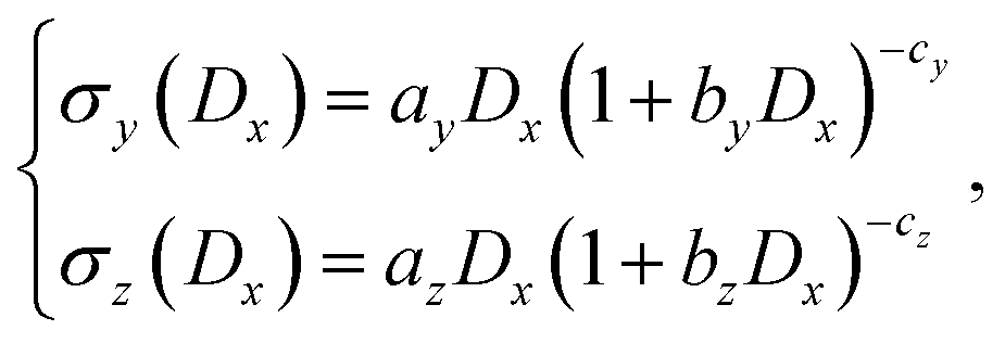 | (4) |
| Terrain | Class of atmospheric stability | ay | by | cy | az | bz | cz |
|---|---|---|---|---|---|---|---|
| Urban | A and B | 0.32 | 0.0004 | −0.5 | 0.24 | 0.001 | −0.5 |
| C | 0.22 | 0.0004 | −0.5 | 0.2 | 0 | −0.5 | |
| D | 0.16 | 0.0004 | −0.5 | 0.14 | 0.0003 | −0.5 | |
| E and F | 0.11 | 0.0004 | −0.5 | 0.08 | 0.0015 | −0.5 | |
| Open country | A | 0.22 | 0.0001 | −0.5 | 0.2 | 0 | −0.5 |
| B | 0.16 | 0.0001 | −0.5 | 0.12 | 0 | −0.5 | |
| C | 0.11 | 0.0001 | −0.5 | 0.08 | 0.0002 | −0.5 | |
| D | 0.08 | 0.0001 | −0.5 | 0.06 | 0.0015 | −0.5 | |
| E | 0.06 | 0.0001 | −0.5 | 0.03 | 0.0003 | −1 | |
| F | 0.04 | 0.0001 | −0.5 | 0.16 | 0.0003 | −1 |
The training data of the ANN are generated by following workflow:
(1) Define the range of the training area (ranges of x, y and z);
(2) Define all possible atmospheric stabilities and terrains;
(3) Define the range of the ANN input parameters;
(4) Randomly generate sampling points in the training area;
(5) Use atmospheric dispersion models to calculate the ANN output;
(6) Generate input and target data for training and validation sets.
In each scenario, as can be seen in Table 4, the release rates q of all possible emission sources vary from 0 to 5 g s−1. The wind speed v varies from 0 to 5 m s−1. The wind direction satisfies that d ∈ {x|0 < x ≤ 360,x ∈ Z}. In order to cover a wider range of environmental conditions, ten different typical combinations of diffusion coefficients are selected to simulate the dispersion process (shown in Table 3). Table 3 indicates the relationship between diffusion coefficients and atmospheric stability according to Carrascal et al.33 After using these scenarios to simulate the atmospheric dispersion process, we can then obtain the numerical concentrations measured at sampling points randomly distributed in [xmin,xmax] and [ymin,ymax]. Moreover, we assume that the UAV platform moves at a constant height h and the number of sampling points is Ts. According to Section 2.2.1, we have four or five input ANN parameters. Because the flight height is a constant value (50 m), it is not necessary to consider the input parameter z in Fig. 2. Therefore, the input layer of the ANN has four neurons. Furthermore, the number of neurons in the output layer equals the number of candidate sources since it is a classification ANN. It can be seen that there are only five candidate SO2 emission sources in Table 1, so the output layer has five neurons. Because the detailed training procedure is beyond the research scope of this paper, the ANN will be directly trained by the MATLAB neural network toolbox.34
| Parameter | Explanation | Value |
|---|---|---|
| d | Wind direction (degree) | 1–360 with step 1 |
| v | Wind speed (m s−1) | 1–5 with step 2 |
| q | Release rate (g s−1) | 1–5 with step 2 |
| ay,by,cy | Parameters of σy | See Table 3 |
| az,bz,cz | Parameters of σz | See Table 3 |
| xmin | Lower bound of training area x-axis (m) | −2000 |
| xmax | Upper bound of training area x-axis (m) | 2000 |
| ymin | Lower bound of training area y-axis (m) | −1000 |
| ymax | Upper bound of training area y-axis (m) | 3000 |
| h | Flight altitude (m) | 50 |
| Ts | Number of sampling point for each release | 100 |
As shown in Table 4, we have 360 × 3 × 3 × 10 = 32![[thin space (1/6-em)]](https://www.rsc.org/images/entities/char_2009.gif) 400 different virtual scenarios. Since each scenario has 100 sampling points, we can obtain 32400 × 100 = 3240000 sets of data, 75% of which are for training and 25% of which are for validation. The average correct rate (ACR) of the training data is 83.05% and that of the validation data is 82.09%. Furthermore, the comparison between the ANN output and training/validation results is shown in Fig. 5. As can be seen from the figure, the ANN output (weight of optimal source) closely matches the training targets and validation targets, the mean square errors (MSE) of which are 0.089 and 0.123 respectively.
400 different virtual scenarios. Since each scenario has 100 sampling points, we can obtain 32400 × 100 = 3240000 sets of data, 75% of which are for training and 25% of which are for validation. The average correct rate (ACR) of the training data is 83.05% and that of the validation data is 82.09%. Furthermore, the comparison between the ANN output and training/validation results is shown in Fig. 5. As can be seen from the figure, the ANN output (weight of optimal source) closely matches the training targets and validation targets, the mean square errors (MSE) of which are 0.089 and 0.123 respectively.
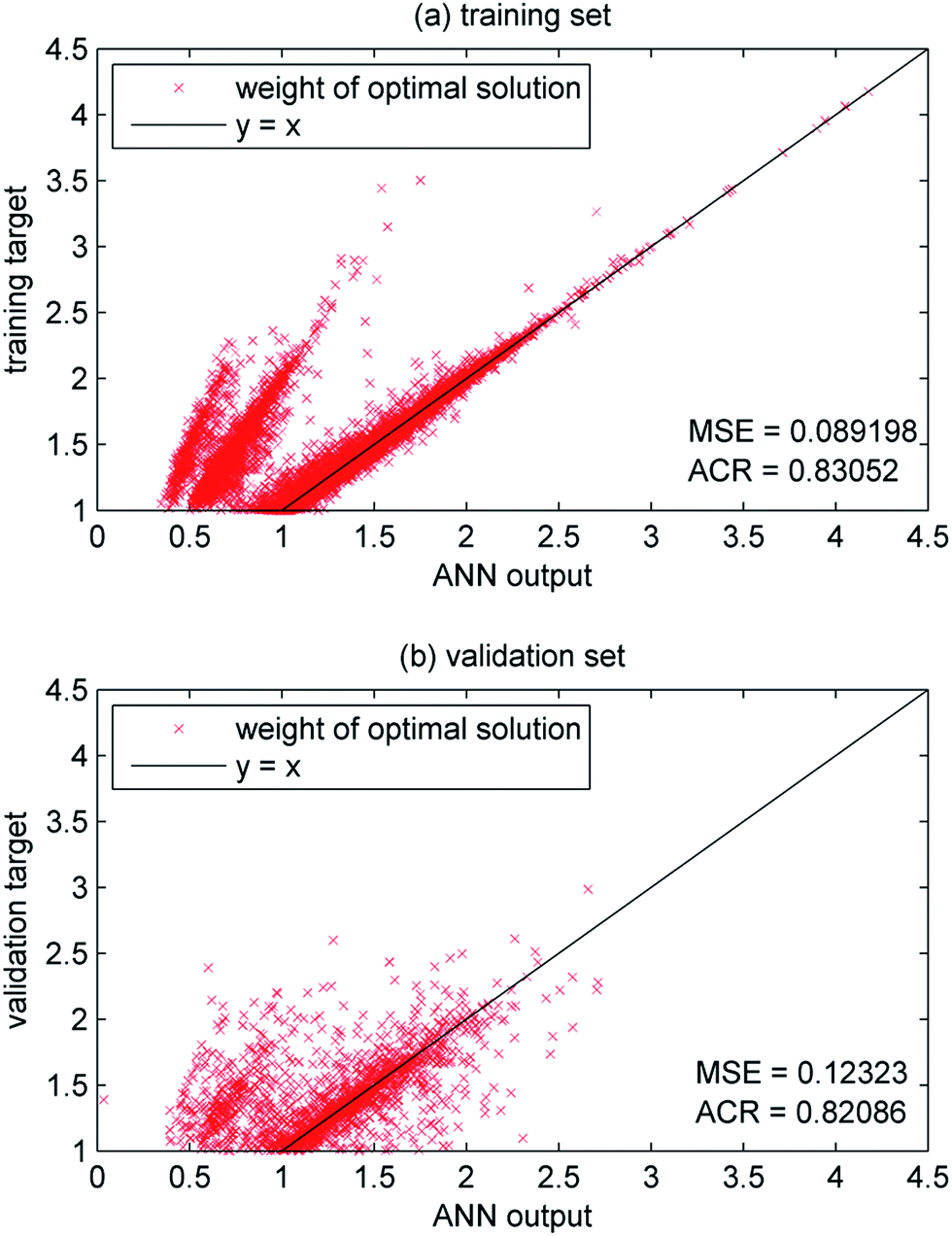 | ||
| Fig. 5 Comparison of ANN output and training/validation target. | ||
3 Experimental
3.1 Numerical experiment
A simulated numerical experiment is quite appropriate for testing the performances of most features of the proposed approach, because it is easier to set the parameters or variables in numerical experiments. In the numerical experiment, we analyse the performance of the ANN based source estimation method. Furthermore, the source estimation methods based on Bayesian inference and optimization are also used for comparison.The source estimation method based on Bayesian inference is quite simple in this experiment because there are only five candidate sources. Thus, it is unnecessary to use a posterior distribution sampling algorithm (such as MCMC) in this experiment. After calculating the posterior probabilities of the five potential sources, the candidate source with the highest posterior probability is considered as the optimal solution.
In the optimization method, the cost function is defined as follows:
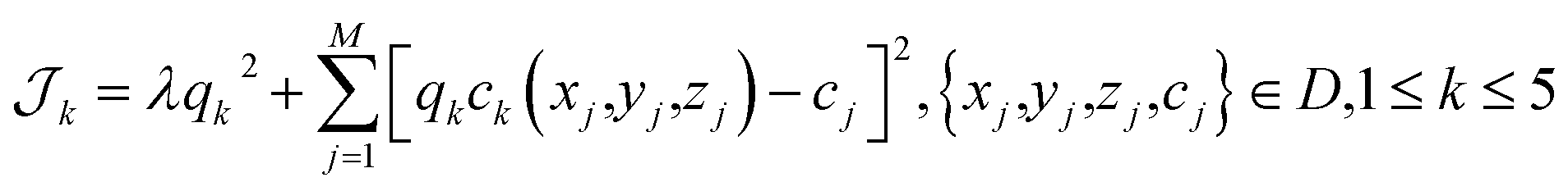 | (5) |
 . These cost functions can be minimized by Tikhonov regularization through adjusting the variable qk. The candidate source with the minimum value of the cost function is the estimated emission source.
The numerical experiment requires these three methods to estimate the SO2 emission source using concentration data generated by the KD-ADSS simulation tool. In order to test the accuracy and stability of the source estimation approaches, the wind direction varies from 0 to 360° for all test cases. The wind speed is 3.7 m s−1 and the release rate is 4.1 g s−1. To test the effect of environmental conditions, the diffusion coefficients σy and σz also vary during the test. Their expressions are as follows:
 | (6) |
Noise sources are added into the concentration measurements, wind direction, and diffusion coefficient in each test case to test the stability of the proposed method. The noise sources follow Gaussian distributions N(0,σ2). For the concentration noise ec, the equation of its deviation σc is σc = fcc, where c is the value of the measured concentration and fc is the noise coefficient, which increases from 0 to 0.5. For the wind direction noise ed, its deviation σd increases from 0 to 30. The noise of the diffusion coefficient follows a simple Gaussian distribution whose deviation is 0.1σx or 0.1σy. All the control variables in the numerical experiment are shown in Table 5.
| Control variable | Range |
|---|---|
| Wind direction d | 0 to 360 (deg) |
| Concentration noise coefficient fc | 0 to 0.5 |
| Wind direction noise coefficient (deviation) σd | 0 to 30 (deg) |
| Atmospheric stability noise coefficient fp | 1 to 4 |
The flight route of the UAV is shown in Fig. 4, in which the moving velocity remains steady at 10 m s−1. The sensors sample the concentration data once per second. After using the simulation tool to calculate the SO2 concentrations of each scenario, the neural network, Bayesian inference and optimization methods are applied to test their performances.
3.2 Real experiment
After obtaining permission from the committee of the chemical industry park, a real experiment was conducted on 27th May, 2016 in Shanghai. This experiment used ZE-03 SO2 sensors produced by Weisheng Inc. This real experiment was conducted in the same location introduced in Section 2.3. The aircraft took off and moved around the chemical industry park. When the aircraft arrived at the south-west corner, we found that the concentration of SO2 increased rapidly and soon reached its peak. At this location, the aircraft was manually controlled to turn around through the SO2 plume several times to sample sufficient data. According to our observation and investigation, the chimney of the sulfuric acid recovery (SAR) system was the only location from which SO2 gas was emitted during this time. As a result, we could be sure that the chimney of the SAR system was the emission source that caused the increase of the SO2 concentration. In addition, noise was added to the concentration and wind data to test the stability of the models.4 Results and discussions
4.1 Results of numerical experiment
The source estimation approach is applied in each test case of the numerical experiment and the results are presented in Fig. 6. These figures show the ACR of the ANN, Bayesian inference (maximum posterior probability) and optimization (minimum cost function). Fig. 6(a) shows the relationship between the ACR and wind direction d when d increases from 0 to 360°. The other parameters are: fc = 0.1, σd = 5, and fp = 1. As can be seen in this figure, the ACR curves of the ANN, Bayesian inference and optimization have similar trends. The ACR of the ANN (77.38%) is clearly higher than that of Bayesian inference (74.56%) and optimization (72.17%). When the wind direction satisfies that d ∈ (120,180)∪(300,360), the correct rates of these three methods are quite high (nearly 100%). However, when the wind direction d is not in this range, the correct rates of ANN, Bayesian inference and optimization fluctuate between approximately 50–90%, 40–90% and 20–90% respectively. Therefore, the performance of the ANN is better than Bayesian inference and optimization. It is worth mentioning that some candidate sources may generate very similar measurements in some directions. Thus, the tested methods may therefore mistakenly identify the wrong source, which is also the reason for some obvious errors appearing in the ANN training results in Fig. 5. To address this problem, turning the aircraft around several times to sample more data or re-designing a more effective flight route may improve the results.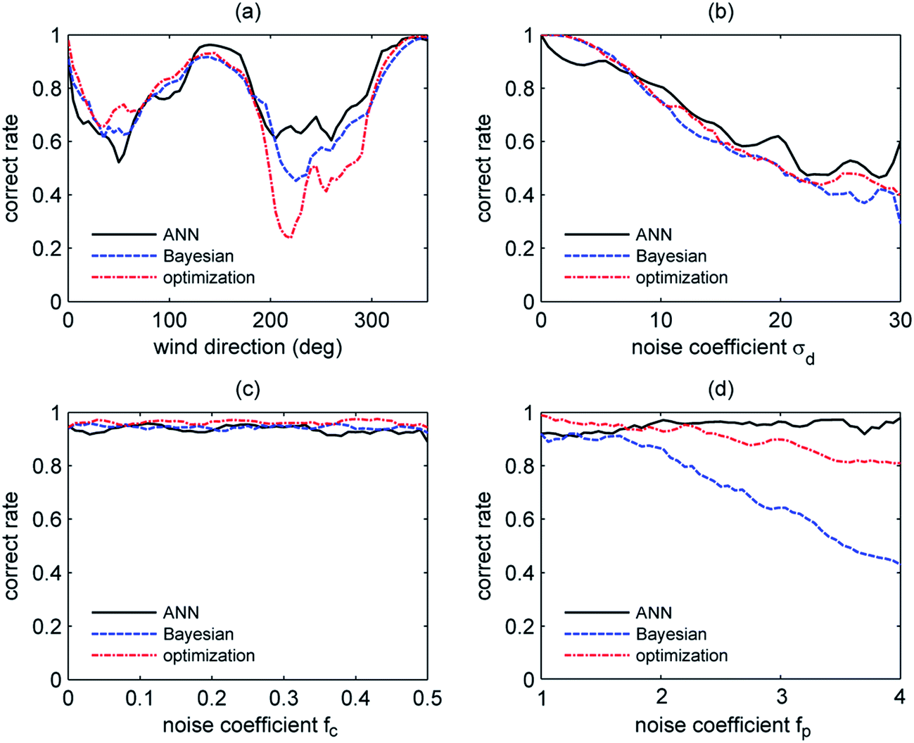 | ||
| Fig. 6 Results of numerical experiment: (a) Effect of wind direction d. (b) Effect of noise deviation of wind direction σd. (c) Effect of noise coefficient of concentration fc. (d) Effect of atmospheric stability coefficient fp. | ||
Fig. 6(b) shows the effect of the noise deviation of wind direction σd when d = 0, fc = 0.1 and fp = 1. As we can see in this figure, when σd is less than 5, the correct rates of Bayesian inference and optimization remain stable at very high accuracy, while that of the ANN experiences a slight decrease. σd when σd is larger than 5, the ACR of the ANN becomes higher than the other two methods. All three methods drop to around 40% with the maximum noise coefficient. Therefore, all three methods are relatively sensitive when noise is added into the wind direction. Consequently, the accuracy of source estimation heavily depends on the accuracy of the meteorological parameters.
Fig. 6(c) illustrates the ACR as a function of the concentration noise coefficient fc when d = 0, σd = 5 and fp = 1. Clearly, the concentration noise has almost no influence on the accuracies of all three methods. The correct rates of the ANN, Bayesian inference and optimization remain stable at around 90%. Therefore, all three source estimation methods are quite stable when noise is added into the concentration data.
In terms of the atmospheric stability coefficient fp, Fig. 6(d) indicates the relationship between fp and the accuracy when d = 0, fc = 1, and σd = 5. The purpose of this case is to test the stability of the source estimation approaches when the environmental conditions (especially atmospheric stability) vary. In the atmospheric dispersion model, Gaussian diffusion coefficients are used for describing the atmosphere stability. Therefore, we use eqn (5) to set a series of test cases with different atmospheric stabilities. fp = 1 represents the atmospheric condition of class D in open country. fp = 4 represents that the atmosphere is extremely unstable. As we can see in Fig. 6(d), the estimation approach based on the ANN is quite robust when the atmospheric stability varies. However, the accuracy of Bayesian inference significantly decreases during this test, dropping to only 40% when fp = 4. The optimization method also shows a downward trend, finally falling to 80%.
Therefore, noise sources in both wind direction and concentration have similar effects on these three methods with the accuracy of the ANN being slightly higher. When it comes to atmospheric stability, the advantage of the ANN becomes much more obvious. The most important reason that we use the ANN is to bypass the effect of atmospheric stability. The experimental results show that the ANN can effectively meet our requirement.
To further analyze the features of the proposed approach, we test the performances of the source estimation methods as a function of atmospheric stability in all possible wind directions when d = 0, σd = 5 and fc = 0.1 (presented in Fig. 7). It is clear that the performance of the ANN remains good in different atmospheric stabilities at all times, while the accuracy of Bayesian inference becomes significantly lower if the atmosphere becomes unstable. Because of the penalty term in the cost function, the correct rate of optimization drops by at most 40% and its performance is slightly better than Bayesian inference.
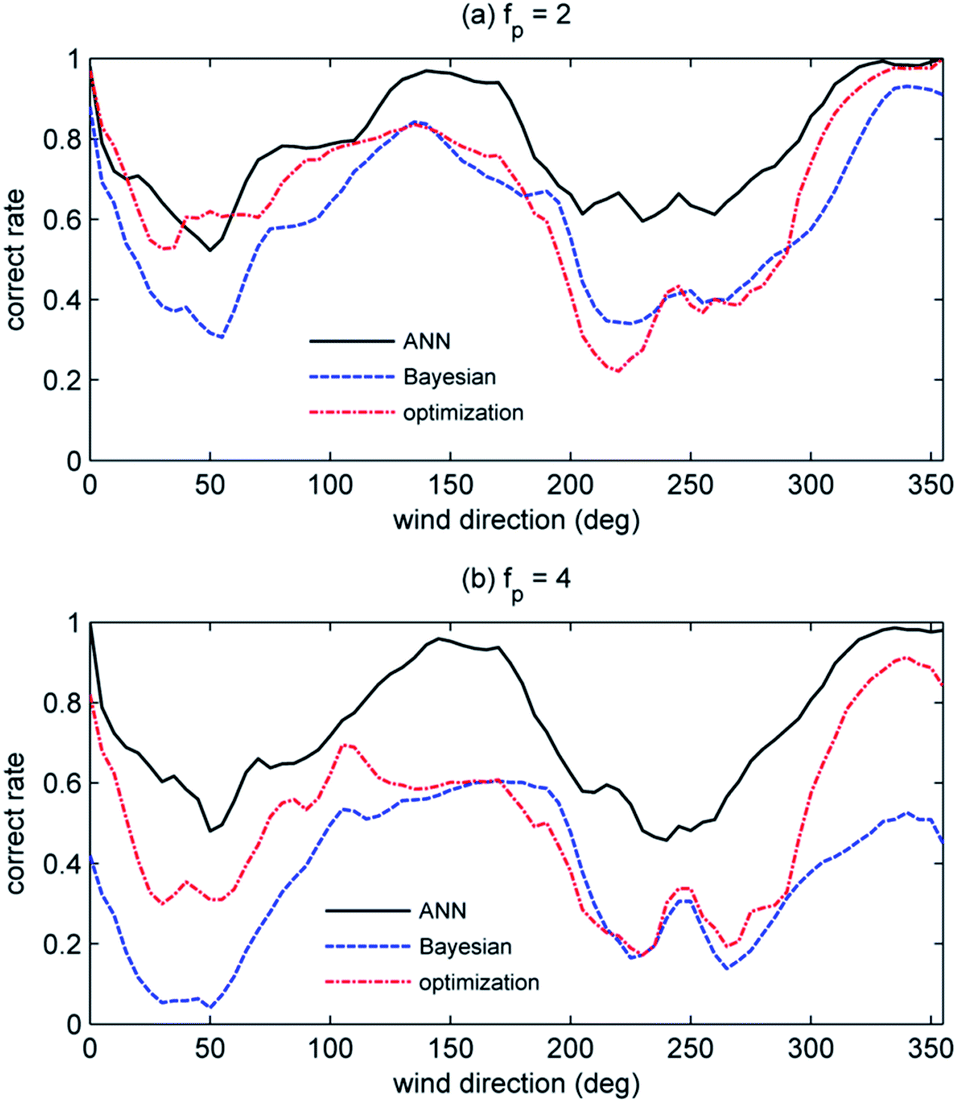 | ||
| Fig. 7 Correct rate of ANN, Bayesian inference and optimization when (a) fp = 2 and (b) fp = 4. | ||
Generally, the atmospheric stability is very difficult to quantify, while other parameters such as wind direction and concentration can be easily measured. Therefore, determining the precise atmospheric stability as well as the diffusion coefficient is a troubling issue in traditional methods like Bayesian inference and optimization. Fortunately, the source estimation approach based on an ANN can address this problem effectively, which makes it highly promising in real applications.
4.2 Results of real experiment
The measurements of the real experiment are shown in Fig. 8. When the aircraft arrived at the south-west corner, the measured concentration dramatically increased. Therefore, the aircraft was manually controlled to fly forwards and backwards over the south-west corner several times in order to sample sufficient dominant data. Fig. 8(a) represents the measured concentrations sampled by the UAV platform. As we can see in this figure, the aircraft spent most of its time flying around the south-west corner (data no. 300 to no. 1200) and the highest concentration reached almost 16 mg m−3.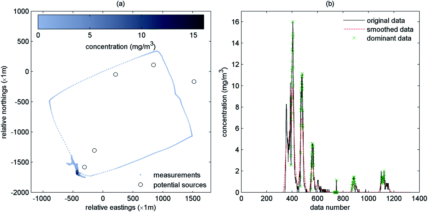 | ||
| Fig. 8 The SO2 measurements of the real experiment: (a) Flight route and measured concentration are shown as a scatter plot. (b) Original concentration data, smoothed data, and selected dominant data. | ||
Via the method introduced in Section 2.2, the original measurements are smoothed by a linear average filter. Thus, the dominant data are then selected according to the proposed method in Section 2.2. The smoothed SO2 concentration data and dominant data are displayed in Fig. 8(b) together with the original data. According to Fig. 8(b), the dominant data contain six dominant subsets. The average wind directions and wind speeds of all dominant subsets are presented in Table 6. Thus, the trained ANN is applied to calculate the output from these data (shown in Fig. 9). All of these input subsets result in the same conclusion – “chimney of SAR system” is the estimated emission source according to the sum of each output.
| Dominant subset ID | Average wind direction (deg) | Average wind speed (m s−1) |
|---|---|---|
| 1 | 81.7 | 1.9 |
| 2 | 90.5 | 3.4 |
| 3 | 85.3 | 4.2 |
| 4 | 103.7 | 4.4 |
| 5 | 105.5 | 1.7 |
| 6 | 102.8 | 2.9 |
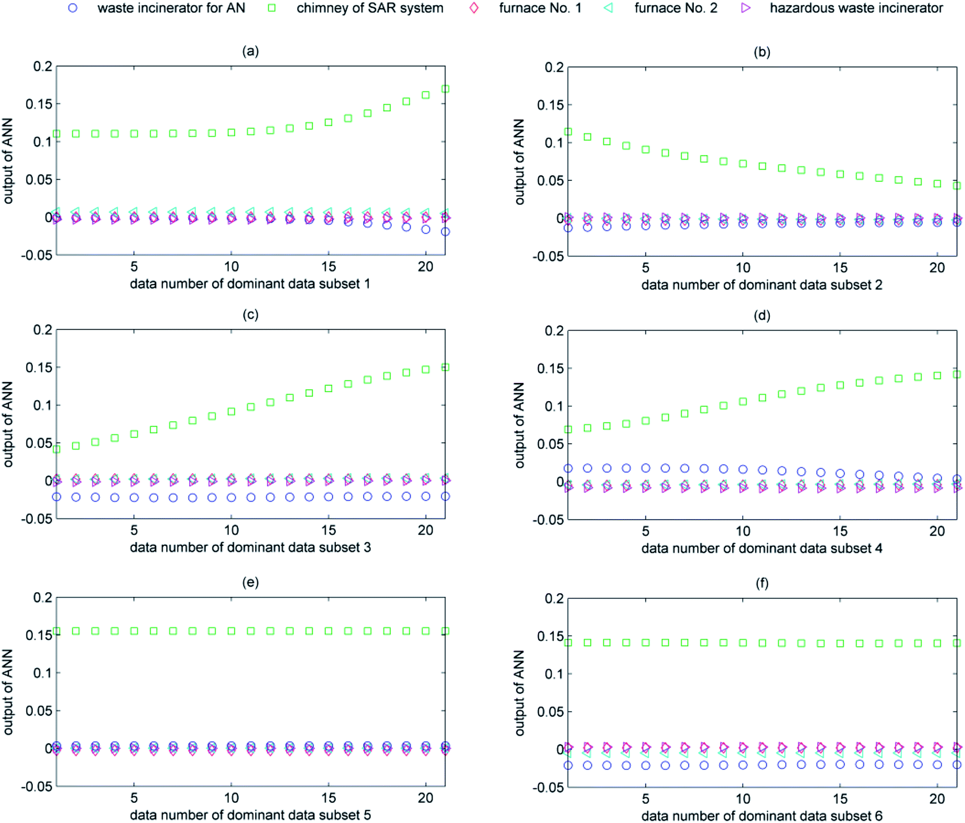 | ||
| Fig. 9 The neural network output of six dominant subsets. | ||
To test the sensitivity in real situations, virtual noises are added into the input variables to study the resulting uncertainty of the output. Because atmospheric stability is quite difficult to measure, we only test the sensitivity of the proposed method to changes in wind direction, wind speed and concentration. The virtual noises include wind direction noise ed, wind speed noise ev and concentration noise ec, following the normal distributions ed ∼ N(0,σd), ev ∼ N(0,σv) and ec ∼ N(0,fcc) respectively. The effect of wind direction is shown in Fig. 10 when σv = 1 and fc = 0.1. As can be seen from the figure, if the deviation of wind direction satisfies σd ≤ 12°, the accuracy is quite high and the ACR remains stable at almost 100%. If σd > 12°, the ACR begins to decline gradually, decreasing to around 50% when σd reaches 30°. We can therefore conclude that the stability of the proposed method with respect to wind direction is acceptable in practice. In terms of wind speed, the sensitivity analysis result shows that the ACR remains unchanged at 100% when the deviation of wind speed noise varies from 0 to 3 m s−1. For the uncertainty in concentration, we find it is unnecessary to plot its sensitivity analysis result because the ACR is always 100% when the noise coefficient of concentration satisfies that 0 ≤ fc ≤ 0.5. In practice, fc = 0.5 is a fairly high concentration noise, which is not common in real sensors. Therefore, the proposed method is extremely insensitive to concentration noise. This confirms that the use of low-price sensors on the UAV platform is acceptable for source term estimation.
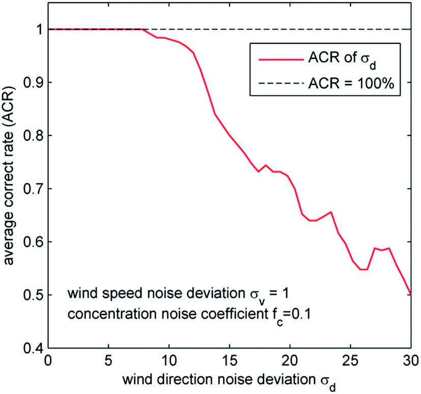 | ||
| Fig. 10 Sensitivity analysis result of wind direction. | ||
5 Discussions
As mentioned in Section 4.1, the accuracy of the source estimation methods may be low in some wind directions. For example, when wind direction d = 15°, the trends of the SO2 air concentration measurements generated by the waste incinerator for acrylonitrile, the chimney of the SAR system, and Furnace no. 1 are quite similar. All of them reach their concentration peaks in the south-west corner. Because the SO2 gas plumes of these potential sources are overlapped at the south-west corner when d = 15°, it is difficult to identify exactly which of them emits the contaminant. To settle this problem, we suggest to re-plan the flight route to sample dominant data containing more useful information. An effective flight route can avoid ambiguity of identification. For example, Fig. 11 shows an alternative flight route of the UAV platform and Fig. 12 shows its identification results. Clearly, changing the original flight route can greatly improve the accuracy (the mean correct rate is 87.64%).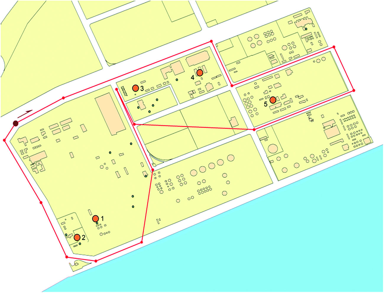 | ||
| Fig. 11 An alternative, improved flight route for contaminant concentration sampling. | ||
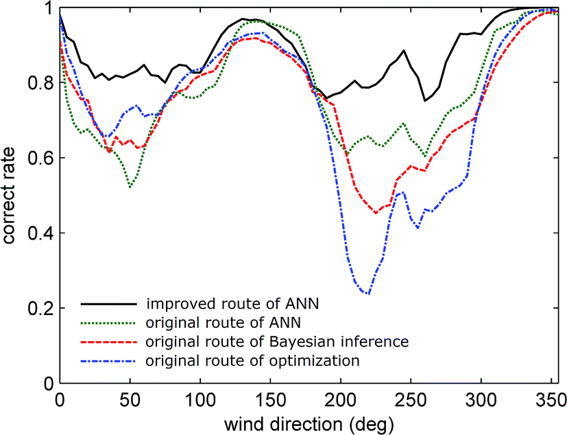 | ||
| Fig. 12 Source estimation results of ANN, Bayesian inference, optimization and ANN with the improved route. | ||
However, planning the flight route is a complex task, and is not the focus of our current research work. Furthermore, the flight route also has some restrictions. For example, some facilities may be too dangerous for the aircraft to fly over them. Therefore, designing an effective flight route is an important but challenging task.
The numerical experiment compares the ANN-based source estimation approach with methods based on Bayesian inference and optimization. The source estimation approach based on the ANN is more stable in changing environmental conditions. The ACR of this approach demonstrates almost no change (as shown in Fig. 7) when the atmospheric stability coefficient is changed from 1 to 4 (stable to unstable). Atmospheric stability and other complex meteorological parameters that are used in Bayesian inference and optimization cannot be precisely measured. However, the ANN-based approach is able to bypass these parameters. In terms of the effect of wind direction, the ACR of the ANN-based approach (77.38%) is higher than those of Bayesian inference and optimization (74.56% and 72.17% respectively) because it has been trained on pre-determined scenarios. In the training set, the ACR of the ANN is 83.05%, and the ACR in the validation set is only slightly lower (82.08%). A well-trained ANN is the basis of accurate inverse calculation, which makes the ANN-based approach the optimal option for source estimation in chemical industry parks. The weak point of the ANN is that the investigation area must be pre-determined, because the source estimation approach based on the ANN needs a large number of training data sampled from this area. Moreover, the number of candidate sources cannot be too large and the ANN cannot identify multiple sources, which are disadvantages that it shares with other traditional methods. However, in chemical industry parks, it is easy to obtain detailed information of the scenario and candidate sources, which means that the ANN method is quite suitable for daily monitoring and management of chemical industry parks.
The real experiment implemented the source estimation method using real SO2 concentration data. The proposed approach was also verified by the observed and investigated results. Because of the flexibility of the UAV platform, the remote monitoring system was able to sample data containing useful information. The experimental results show that the ACR concerning wind direction is quite high when the error deviation is less than around 12°. Furthermore, the presence of noise in the wind speed and concentration data has almost no influence on the accuracy: the ACR remains at 100% at all times when these noise sources vary within realistic ranges. Although the resolution and accuracy of the sensors installed on the UAV platform (ppb or ppm level) were much lower than those of static sensors (ppt or ppb level), the proposed method was acceptably insensitive to the measurement errors. Consequently, the real experiment illustrates the advantages of the source estimation approach based on an ANN and a UAV platform and demonstrates that this approach can be successfully applied in a real chemical industry park.
6 Conclusion
This paper proposed an approach for estimating a contaminant dispersion source based on a UAV platform, an ANN and an atmospheric dispersion simulation tool. Using a UAV platform can overcome the limitations of static sensors and allow the sampling of high-quality concentration data containing important spatial information. Using an ANN can bypass the need for complex parameters and mechanisms of backward calculation and provide stability when the environmental conditions change dramatically. Because this platform is insensitive to noise added into the concentration measurements, it is feasible to install gas sensors that are relatively inaccurate but lightweight. However, noise in the wind direction data can significantly influence the final accuracy. The meteorological data should therefore be of high accuracy and precision, in agreement with the conclusions of previous studies. Furthermore, planning an effective flight route is an important measure to promote the accuracy of source estimation.The approach proposed in this paper had a positive impact in practice. A more advanced monitoring system is now under development. The gas sensors have been upgraded to the μg m−3 level. In addition, Raspberry Pi has been replaced by a stable micro-controller. In terms of the source estimation approach, the current version is only appropriate for single-source identification. Therefore, a multi-source identification algorithm will be investigated in the future.
Conflicts of interest
There are no conflicts to declare.Acknowledgements
This study is supported by National Key Research & Development (R&D) Plan of China under Grant No. 2017YFC0803300, the National Natural Science Foundation of China under Grant No. 71673292 & 61503402, Guangdong Key Laboratory for Big Data Analysis and Simulation of Public Opinion and Shanghai Special Foundation of Software and Integrated Circuit under Grant No. 150312.References
- Y.-S. Chung, S.-H. Kim, J.-H. Moon, Y.-J. Kim, J.-M. Lim and J.-H. Lee, J. Radioanal. Nucl. Chem., 2006, 267, 35–48 CrossRef CAS.
- G. Katata, M. Chino, T. Kobayashi, H. Terada, M. Ota, H. Nagai, M. Kajino, R. Draxler, M. C. Hort, A. Malo, T. Torii and Y. Sanada, Atmos. Chem. Phys., 2015, 15, 1029–1070 Search PubMed.
- A. Keats, E. Yee and F.-S. Lien, Atmos. Environ., 2007, 41, 465–479 CrossRef CAS.
- E. Lushi and J. M. Stockie, Atmos. Environ., 2010, 44, 1097–1107 CrossRef CAS.
- V. Winiarek, J. Vira, M. Bocquet, M. Sofiev and O. Saunier, Atmos. Environ., 2011, 45, 2944–2955 CrossRef CAS.
- M. Hutchinson, H. Oh and W.-H. Chen, Inform. Fusion, 2017, 36, 130–148 CrossRef.
- N. A. Gatsonis, M. A. Demetriou and T. Egorova, 2015 IEEE International Symposium on Technologies for Homeland Security (HST), 2015, pp. 1–6 Search PubMed.
- B. Hirst, P. Jonathan, F. González del Cueto, D. Randell and O. Kosut, Atmos. Environ., 2013, 74, 141–158 CrossRef CAS.
- M. L. Melamed, S. Solomon, J. S. Daniel, A. O. Langford, R. W. Portmann, T. B. Ryerson, J. D. K. Nicks and S. A. McKeen, J. Environ. Monit., 2003, 5, 29–34 RSC.
- T. Mori, T. Hashimoto, A. Terada, M. Yoshimoto, R. Kazahaya, H. Shinohara and R. Tanaka, Earth, Planets Space, 2016, 68, 1–18 CrossRef.
- Y. Sanada and T. Torii, J. Environ. Radioact., 2015, 139, 294–299 CrossRef CAS PubMed.
- A. Sinha, A. Tsourdos and B. White, IFAC Proceedings Volumes, 2009, 42, 7–12 CrossRef.
- B. White, A. Tsourdos, I. Ashokaraj, S. Subchan and R. Zbikowski, in AIAA Guidance, Navigation and Control Conference and Exhibit, American Institute of Aeronautics and Astronautics, 2007, DOI:10.2514/6.2007-6761.
- Z.-R. Peng, D. Wang, Z. Wang, Y. Gao and S. Lu, Atmos. Environ., 2015, 123, 357–369 CrossRef CAS.
- S. K. Rao, Atmos. Environ., 2007, 41, 6964–6973 CrossRef.
- M. Borysiewicz, A. Wawrzynczak and P. Kopka, Foundations of Computing and Decision Sciences, 2012, 37, 253 CrossRef.
- E. Yee, presented in part at the Chemical and Biological Sensing VIII, ed. W. Fountain Augustus III, Proceedings of the SPIE, 2007 Search PubMed.
- L. Tierney, Ann. Statist., 1994, 22, 1701–1728 CrossRef.
- T. M. Chin and A. J. Mariano, J. Atmos. Ocean. Tech., 2010, 27, 371–384 CrossRef.
- A. Wawrzynczak, P. Kopka and M. Borysiewicz, presented in part at the Parallel Processing and Applied Mathematics: 10th International Conference, Berlin, Heidelberg, 2014, pp. 407–417 Search PubMed.
- Y. Zhang and L. Wang, Advanced Technology in Teaching: Selected papers from the 2012 International Conference on Teaching and Computational Science (ICTCS 2012), 2013, pp. 517–523, DOI:10.1007/978-3-642-29458-7_76.
- X. L. Zhang, G. F. Su, H. Y. Yuan, J. G. Chen and Q. Y. Huang, J. Hazard. Mater., 2014, 280, 143–155 CrossRef CAS PubMed.
- D. Ma, S. Wang and Z. Zhang, Atmos. Environ., 2014, 94, 637–646 CrossRef CAS.
- S. Qiu, B. Chen, Z. Zhu, Y. Wang and X. Qiu, J. Radioanal. Nucl. Chem., 2016, 1–14, DOI:10.1007/s10967-016-4941-z.
- V. M. Krasnopolsky and H. Schiller, Neural Networks, 2003, 16, 321–334 CrossRef PubMed.
- V. Vukovic, P. C. Tabares-Velasco and J. Srebric, J. Air Waste Manage. Assoc., 2010, 60, 1034–1048 CAS.
- B. Wang, B. Chen and J. Zhao, J. Hazard. Mater., 2015, 300, 433–442 CrossRef CAS PubMed.
- W. So, J. Koo, D. Shin and E. S. Yoon, Comput.-Aided Chem. Eng., 2010, 28, 199–204 CAS.
- K. Akahane, S. Yonai, S. Fukuda, N. Miyahara, H. Yasuda, K. Iwaoka, M. Matsumoto, A. Fukumura and M. Akashi, Environmentalist, 2012, 32, 136–143 CrossRef.
- X. Feng, Q. Li, Y. Zhu, J. Hou, L. Jin and J. Wang, Atmos. Environ., 2015, 107, 118–128 CrossRef CAS.
- DJI. Inc., Matrice 100-Specifications, http://wiki.dji.com/en/index.php/Matrice_100-Specifications, accessed 11 August, 2016.
- Raspberry PI, Raspberry Pi 2 Model B, http://www.raspberrypi.org/products/raspberry-pi-2-model-b/.
- M. D. Carrascal, M. Puigcerver and P. Puig, Theor. Appl. Climatol., 1993, 48, 147–157 CrossRef.
- MATLAB, Version 7.11.0, The MathWorks Inc., Natick, Massachusetts, 2010 Search PubMed.
| This journal is © The Royal Society of Chemistry 2017 |