
 Open Access Article
 This Open Access Article is licensed under a
 Creative Commons Attribution 3.0 Unported Licence
Study on the fractal characteristics of rock in the prediction of rockburst
Li Mo-xiao *,
Song Ying-hua* and
Zhang Guang*
*,
Song Ying-hua* and
Zhang Guang*
Wuhan University of Technology, Wuhan, China. E-mail: lmx@whut.edu.cn; song6688c@163.com; gzhang58@163.com
First published on 5th September 2017
Abstract
In order to strengthen the forecasting of rockburst in underground engineering, the fractal characteristics of the rockburst proneness of rock were studied in this paper. The fractal characteristics of rock surface and acoustic emission were analyzed based on four types of rocks by uniaxial compression testing. The changes in fractal characteristics among the different types of rock were compared by calculating the geometric dimension and acoustic emission dimension. Results showed that the rock with stronger rockburst proneness had more intensive failure in the loading process.
1. Introduction
With the great progress of social economy, underground engineering has gradually been developed more and more deeply. On this background, rockburst has become one of the major geological disasters limiting the development of underground engineering. Rockburst is a nonlinear dynamic phenomenon in which a rock mass releases energy extremely rapidly along the excavation free face.1 Rockburst is a complicated problem and there is neither a set of mature theories on its prediction nor comprehensive understanding of the cause of its formation. Some scholars believe that rockburst is a unique property of the rock itself, which is inherently determined by the rock's physical condition.2 This research was conducted from the angle of rockburst proneness. In the course of the study, theory based on the traditional Euclidean space suffered limitations to a certain extent. In 1987, Xie Heping began to use the fractal characteristics of rock in his doctoral thesis, and carried out further studies on the application of fractal theory in rock mechanics in 1988–2003, with concentration on the fractal dimension of rock fracture, and the relationship between fractal characteristics and damage and energy dissipation of burst fracture. Then, fractal geometry was introduced to the analysis of rock damage and fracture, including microscopic fracture of rock, macroscopic fracture dynamic expansion and fragmentation distribution of rock mass.3,4 The acoustic emission (AE) phenomenon in the process of failure also shows fractal characteristics. The change of fractal dimension of rock during the deformation process was in concert with its stress state, and mechanical, physical and chemical properties.5 In addition, some scholars believe that rockburst is the result of internal crack propagation; therefore the rockburst mechanism can be further understood by studying the development of cracks during the rock failure process. The fractal theory is an important method to study the development of cracks. More and more scholars use the fractal method to study rockburst. However, as it has been a short time since fractal theory was used in the study of rock mechanics, and no systematic theoretical basis has been formulated, it is difficult to study the rockburst mechanism. In such context, it is of great significance to study rockburst proneness based on fractal characteristics and predict rockburst by establishing a corresponding index. In this paper, uniaxial compression experiments were carried out based on 4 different rocks, namely marble, granite, hornstone and skarn. The changes of a rock's surface fractal dimension and AE dimension were studied by determining and analyzing the surface characteristic of rock before and after testing. Based on this, the relationship between fractal characteristics and rockburst proneness was studied. The mechanism of rock with rockburst proneness is the key problem to be urgently addressed for underground engineering disaster prevention.2. Experiment on rockburst proneness
In order to study the surface fractal characteristics of different rocks, uniaxial compression testing was conducted using marble, granite, hornstone and skarn. Each sample used in the experiment is a conventional standard cylinder with a size of Ø 50 mm × 100 mm. In this experiment we used burst energy index and elastic deformation energy index to measure the strength of rockburst proneness.6,7 Uniaxial compression testing was conducted using an MTS815.04-type rock mechanics test system developed by Wuhan Institute of Rock and Soil Mechanics, Chinese Academy of Sciences. The equipment is shown in Fig. 1. The value of each rockburst proneness index of each rock was calculated by using MATLAB. The results are shown in Table 1. | ||
| Fig. 1 Rock mechanics and AE test systems. | ||
| Sample | σc/MPa | E/104 MPa | ν | Wcf | Wet | |
|---|---|---|---|---|---|---|
| a σc—uniaxial compression strength; E—elastic modulus; ν—Poisson ratio; Wcf—burst energy index; Wet—elastic deformation energy index. | ||||||
| Marble | DH4 | 54.74 | 3.37 | 0.12 | 1.50 | — |
| DH5 | 53.15 | 4.05 | 0.20 | 1.32 | — | |
| DH8 | 54.84 | 4.19 | 0.17 | 1.06 | — | |
| DH6 | 92.32 | 7.31 | 0.15 | — | 1.91 | |
| DH9 | 83.62 | 7.12 | 0.16 | — | 1.72 | |
| Granite | HB1 | 117.18 | 4.19 | 0.14 | 2.31 | — |
| HB2 | 311.24 | 4.64 | 0.22 | 3.00 | — | |
| HB4 | 189.20 | 4.07 | 0.16 | 1.71 | — | |
| HB6 | 151.34 | 3.78 | 0.42 | — | 6.15 | |
| HB7 | 245.60 | 4.27 | 0.16 | — | 6.17 | |
| Hornstone | JY3 | 109.86 | 7.52 | 0.21 | 1.10 | — |
| JY4 | 84.18 | 10.65 | 0.17 | 2.00 | — | |
| JY8 | 125.61 | 7.84 | 0.15 | — | 5.21 | |
| Skarn | X3 | 97.38 | 0.95 | 0.15 | — | 2.16 |
| X4 | 113.99 | 6.21 | 0.07 | 1.22 | — | |
| X6 | 98.26 | 5.84 | 0.18 | — | 2.17 | |
| X8 | 146.95 | 7.95 | 0.15 | 1.42 | — | |
| X10 | 85.98 | 8.19 | 0.14 | 1.37 | — | |
The strength of rockburst proneness of the four rocks from Table 1 can be arranged in the order: granite > hornstone > skarn > marble.
3. The analysis of rock surface fractal characteristics under uniaxial compression
3.1 The extraction of the surface fractal characteristics of rock
We must take pictures of the four rocks before and after testing. In order to obtain surface features of rock before and after the test, as far as possible, we must adopt a professional digital camera. The pictures we take should have high image definition and uniform brightness, without large areas of shadow. The camera lens should be adjusted perpendicularly to the sample surface to avoid image deformation. In order to ensure the consistency of the images before and after the test, we should place the specimens and camera in the same position.8 During data analysis, we should select pictures at the same position before and after testing to analyze the surface fractal feature, and the selected picture after testing should contain at least one crack. Then, the selected pictures were processed by MATLAB software. Here below we take the analysis process of the marble sample as an example.First, we selected a 64 × 64 pixel of rock surface image at the same position before and after testing, wherein the image after testing contains one crack at least, as shown in Fig. 2. To eliminate unwanted information from the picture and facilitate software calculations, the image after extraction was converted into a binary image after adjustment and noise reduction, so that the fractal dimension can be calculated by MATLAB8.0. The specific operations are show in Fig. 3.
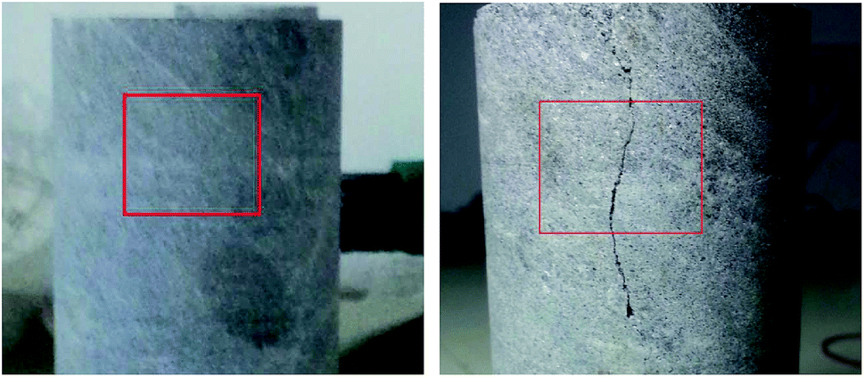 | ||
| Fig. 2 The position of surface feature extraction before and after testing of marble. | ||
 | ||
| Fig. 3 The processing of images after extraction. | ||
3.2 The calculation of fractal dimension of rock before and after testing
Fractal dimension is at the core of fractal theory, which overcomes the limitation of traditional Euclidean geometry. At present, the common method of calculating the fractal dimension is the box counting dimension, also known as box dimension. The calculation formula of box dimension is as follows:
 | (1) |
Specific calculation steps are as follows:
(1) Conduct binarization of images and obtain a binarization data matrix which can be analyzed.
(2) Partition the resulting data matrix into several blocks, guaranteeing the number of rows and number of columns of each block are both k. The number of blocks containing 1 (or 0) is denoted as W(k), k = 1, 2, 4, …, 2i, so the number of boxes is W(1), W(2), W(4),…, W(2i).
(3) Fit the data points (log![[thin space (1/6-em)]](https://www.rsc.org/images/entities/char_2009.gif) K, logW(k), k = 1, 2, 4, …, 2i) with a straight line by the least squares method. The negative value D of the slope of the resulting line is the physical dimension of the image.
K, logW(k), k = 1, 2, 4, …, 2i) with a straight line by the least squares method. The negative value D of the slope of the resulting line is the physical dimension of the image.
The images in Fig. 3 are divided by 2 × 2 pixels block, 3 × 3 pixels block,…, 64 × 64 pixels block. W is the number of non-empty square partitions in the graph, and r is measurement scale (the scale of the block). The dimension can be determined by the linear regression of W and r in the double logarithmic coordinate. The value of the dimension is the absolute value of the slope of the line fitting. Calculation results are shown in Fig. 4.
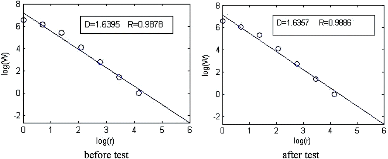 | ||
| Fig. 4 Calculating results of fractal dimension of marble. | ||
Fig. 4 shows that the correlation coefficients of surface fractal dimension fitting of marble before and after testing are generally over 0.98, suggesting that the surface of the rock has fractal characteristics. The above steps were repeated to calculate the dimensions of the other rocks, and the results are shown in Table 2.
| Type | Number | Dimension before test | Dimension after test | Change of dimension | ||
|---|---|---|---|---|---|---|
| Dimension | Average | Dimension | Average | |||
| Marble | DH5 | 1.6391 | 1.6380 | 1.6357 | 1.6450 | 0.0070 |
| DH6 | 1.6538 | 1.6986 | ||||
| DH8 | 1.5998 | 1.5896 | ||||
| DH9 | 1.6590 | 1.6560 | ||||
| Granite | HB6 | 1.6190 | 1.6231 | 1.6611 | 1.6552 | 0.0321 |
| HB7 | 1.6271 | 1.6492 | ||||
| Hornstone | JY4 | 1.6759 | 1.6587 | 1.6540 | 1.6664 | 0.0077 |
| JY8 | 1.6414 | 1.6787 | ||||
| Skarn | X3 | 1.5756 | 1.6272 | 1.6091 | 1.6470 | 0.0198 |
| X6 | 1.6305 | 1.6058 | ||||
| X10 | 1.6756 | 1.6945 | ||||
Table 2 shows that the surface fractal dimensions of the four rocks are all increased after testing. The increase for granite is about 2% and that for skarn is about 1%. The increases for marble and hornstone are both below 1%. The strength of rockburst proneness of the four rocks can be ranked in order as: granite > skarn > hornstone > marble. According to the result, it can be known that the rock of stronger rockburst proneness has a bigger change of dimension between before and after testing. The dimension after testing is bigger than that before testing for the four kinds of rocks. That is because cracks are generated during the uniaxial compressive test, and surface fractal characteristic of a sample will become more complex, leading to a bigger fractal dimension. The rock with stronger rockburst proneness has more intensive failure in the loading process, and its crack morphology is more complex, and thus its change of dimension during the test is bigger. Given all that, the change of dimension during uniaxial compression can be used to judge the strength of rockburst proneness of rock.
4. The characteristics of AE correlation dimension of rock with rockburst proneness
It has been found that the AE parameters of rock also show fractal features. The changes of the four rocks' AE parameters were analyzed by calculating the correlation dimension of time series of AE counts.4.1 G-P method for correlation dimension
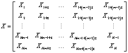
Correlation dimension is calculated by using G-P algorithm. The estimated value of real dimension of the attractor is the correlation dimension of the algorithm.9 The specific calculation steps are as follows, where X is a time series of n:| X = {x1, x2, …, xn} | (2) |
A phase space is constructed according to formula (2). The length of the space is Nm and its dimension is m, wherein m < n. m is defined as the dimension of the reconstructed phase space. The reconstructed phase space is:
 | (3) |
The associated integral function is as follows:
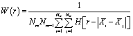 | (4) |
 ; R—observation scale.
Distance between two vectors:
 | (5) |
| C(r) ∝ rD | (6) |
 | (7) |
The scale line of lnr − lnW(r) is the curve of which the vertical coordinate is lnW(r) and horizontal coordinate is lnr. Correlation dimension of time series is the slope of the straight line in the scale-free region of the curve.
4.2 Calculation of AE correlation dimension
The AE signal of rock is generally a one-dimensional time series, which is extremely irregular and complex, with unpredictable and nonlinear characteristics. Correlation dimension is sensitive to the data properties with different AE signals of rock, so that the results will be different.10 In addition, due to the difference in the role of external force, AE signals will be different. Nevertheless, as the statistical regularity of internal defects of materials and activity law of AE belong to one statistical law, there must be some kind of connection between the two.11 Based on the analysis of the count and AE energy during the test, AE fractal features of the four rocks under uniaxial compression were obtained.Due to the large data size in the calculation of correlation dimension, we decided to deal with the calculation with the help of MATLAB. The steps used are as follows:
(1) Determine embedding dimension M and then reconstruct phase space.
(2) Write a command to calculate xi − xj; then we can determine the value of r by using the formula.
(3) The calculation of W(r): write a program according to the Heaviside function to find out the value of  .
.
(4) Fit the resulting points (log(W), log(r)). The fitting results showed that the points were linear, suggesting that the absolute value of the slope of the line is D.
4.3 Analysis of AE correlation dimension of rock with rockburst proneness
The AE correlation dimensions of the four rocks were calculated with the above method. The AE counts and energy parameters of each rock were processed by unary linear regression. The correlation coefficients were more than 0.98, suggesting that the AE parameter series had fractal characteristics and self-similarity in the time domain. The value of AE fractal dimension (D) changed with the stress level, indicating the systematic evolution of rock materials and damage mechanics of rock. Therefore, it can be used to describe the rock mechanics behavior and damage of internal structure.It was found that the correlation dimensions of AE counts of the four rocks at peak strength or before failure were both reduced no matter whether under continuous loading or unloading conditions. The correlation dimensions of AE counts of each specimen are summarized in Table 3.
| Type | Number | Loading mode | Correlation dimension | Average | Reduction of dimension | Average |
|---|---|---|---|---|---|---|
| Marble | DH4 | Continuous loading | 2.6328 | 2.3763 | 0.2786 | 0.2350 |
| DH8 | Continuous loading | 2.8224 | 0.3156 | |||
| DH6 | Unloading | 1.7501 | 0.3442 | |||
| DH9 | Unloading | 2.2999 | 0.0015 | |||
| Granite | HB1 | Continuous loading | 2.4141 | 2.3108 | 1.3499 | 1.0436 |
| HB2 | Continuous loading | 1.8463 | 0.9523 | |||
| HB4 | Continuous loading | 2.1971 | 1.2228 | |||
| HB6 | Unloading | 2.6649 | 1.1044 | |||
| HB7 | Unloading | 2.2731 | 0.7199 | |||
| Hornstone | JY3 | Continuous loading | 2.4652 | 2.2821 | 0.3867 | 0.3039 |
| JY4 | Continuous loading | 2.2609 | 0.4359 | |||
| JY8 | Unloading | 2.2011 | 0.1965 | |||
| Skarn | X4 | Continuous loading | 2.0979 | 2.4867 | 1.0407 | 0.6690 |
| X8 | Continuous loading | 2.6791 | 0.6956 | |||
| X10 | Continuous loading | 2.7703 | 0.1869 | |||
| X3 | Unloading | 2.5583 | 0.2435 | |||
| X6 | Unloading | 2.3568 | 0.6961 |
It can be concluded that the larger the rockburst proneness of a rock, the larger the reduction of AE count correlation dimension of the rock, as shown in Fig. 5. The degree of dimension reduction of the four rocks can be ranked in the order granite > skarn > hornstone > marble. In this way, the degree of dimension reduction of rock is proportional to its rockburst proneness. A rock shows great rockburst proneness when its reduction of dimension is over 40%. Therefore, the reduction of dimension can be regarded as a reference index of rockburst tendency.
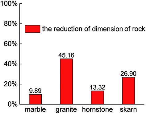 | ||
| Fig. 5 The fractal dimension reduction percentages of four kinds of rocks. | ||
5. Characteristics of AE b-value of rock with rockburst proneness
Ishimoto first proposed the b-value to characterize the relationship between magnitude and frequency of earthquakes in 1993. Then, Gutenberg and other scholars further developed it into practical use. Previously, the b-value was only used in the field of seismic studies. However, it has now been extended to various fields.12 Many scholars considered AE events as earthquake activity or microquakes in the rock damage process, and analyzed the change of b-value under different loading conditions, in order to find out the failure precursor of rock for predicting the rock mass dynamic disaster.13 There is a certain relationship between the fractal characteristics of AE and the change of b-value. The b-value reflects the change of the average intensity and stress of the rock at different times, as well as the scale expansion of microcracks in rock to a certain degree.145.1 AE b-value calculation model
|
logN = a − bm
| (8) |
There are two statistical methods for calculating N according to the particular application, i.e. cumulative frequency and differential frequency.
In cumulative frequency, N is the number of earthquakes (magnitude greater than or equal to m) that have occurred in a certain area. Therefore, such a method is suitable for the prediction of earthquakes occurring in a certain area (magnitude ≥ m).
In differential frequency, N is the number of earthquakes of magnitude range within (m − Δm/2, m + Δm/2). Δm is the magnitude interval which varies with actual situation. This method has good effect in the analysis and interpretation of an earthquake that has already occurred.
This relationship is widely used because of its invariant scale of power exponential function. It can be used to analyze the AE characteristics in the process of rock failure by only replacing the “earthquake” event with AE event.
 | (9) |
lgAi) is the sum of the amplitudes of all the AE events, Ai is the amplitude, ni is the energy of an AE event of which the amplitude is equal to Ai, Am is the minimum amplitude of calculated object, n is the total number of AE events used to calculate the b-value, and e is the base of natural logarithm.155.2 Analysis of AE b-value of rock with rockburst proneness
According to the time series of AE amplitude during uniaxial compression experiments, the b-values of the four rocks in different stages of uniaxial compression testing were calculated by MATLAB. Then the AE b-values of the four rocks under different loading modes were analyzed.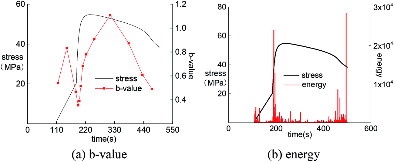 | ||
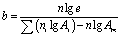
| Fig. 6 Curves of AE b-value and the energy of marble under continuous loading. | ||
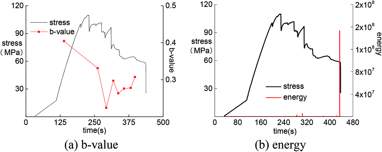
Under load–unload condition (Fig. 7), AE b-value of marble specimen increases along with the decrease of stress during unloading until reaching the loading start point. During the reload process, AE b-value decreases with the increase of stress, reaching the lowest point at peak intensity, before remaining stable. The sudden release of energy before the peak indicates the significant decrease of b-value, and the energy release at stress mutation point after peak is decreased according to the b-value curve.
 | ||
| Fig. 7 Curves of AE b-value and the energy of marble under load–unload condition. | ||
 | ||
| Fig. 8 Curves of AE b-value and the energy of granite under continuous loading condition. | ||
Under load–unload condition (Fig. 9), the b-value of granite keeps decreasing during the period from unloading to reloading to 80% of peak intensity. At 80% of the peak intensity, there is a sudden decline of b-value, and there is an even larger decline of b-value when approaching the peak strength, which corresponds to the AE energy curve. The b-value of the specimen is decreased obviously in production before the peak strength, indicating the formation of through cracks and release of energy.
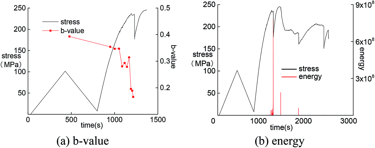 | ||
| Fig. 9 Curves of AE b-value and the energy of granite under load–unload condition. | ||
 | ||
| Fig. 10 Curves of AE b-value and the energy of hornstone under continuous loading condition. | ||
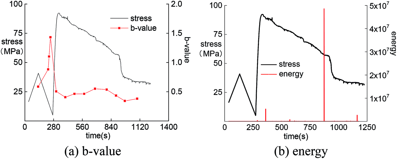
In the process of unloading, the b-value decreases with decreasing stress, wherein the decreasing ranges of the two are similar (Fig. 11). After that in the loading process, the b-value increases firstly and then decreases greatly. After keeping stable for a period, there is a sharp decrease of b-value when approaching the peak strength. This variation process is consistent with the AE energy curve.
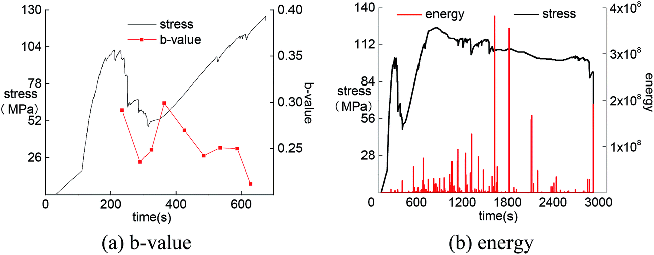 | ||
| Fig. 11 Curves of AE b-value and the energy of hornstone under load–unload condition. | ||
No matter whether under continuous loading or load–unload condition, the b-value always decreases during the period from failure occurrence to the peak strength, which further verifies that the b-value can represent the change in the internal structure of rock.
 | ||
| Fig. 12 Curves of AE b-value and the energy of skarn under continuous loading condition. | ||
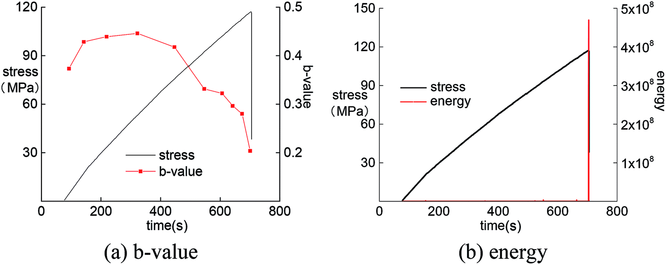
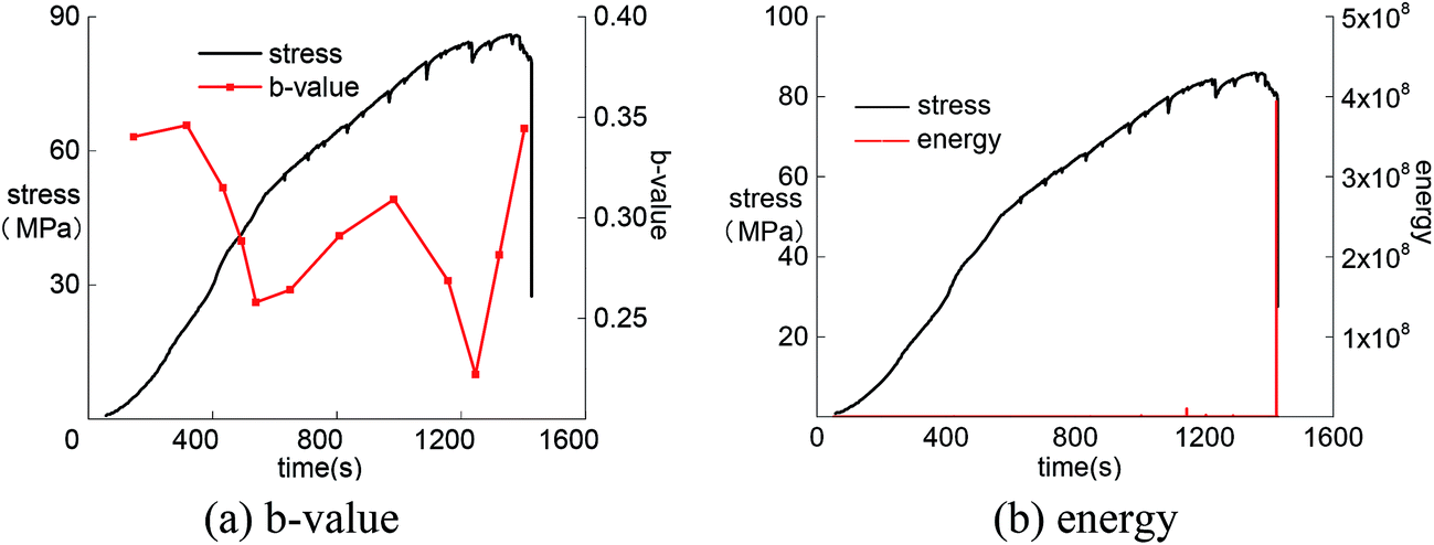
The b-value of skarn under load–unload remains stable at initial loading, and also features a drop before the peak (Fig. 13). After that, there is increase–decrease trend when the reload exceeds the original level, and there is a sharp decrease at the peak intensity, which corresponds to crack propagation and release of internal energy.
 | ||
| Fig. 13 Curves of AE b-value and the energy of skarn under load–unload condition. | ||
By analyzing the change of AE b-value of the four rocks, the reduction of the b-value reveals the release of energy within the specimen. Therefore, the internal damage of rock can be judged by the changing trend of the AE b-value. The AE b-value was generally stable in the early stage but then featured dramatic changes before failure at the peak strength. This means that the growth of microcracks in the early stage is not obvious. With the accumulation of internal energy, the rock was eventually destroyed, releasing a large amount of energy. The b-value can be used as a reference index for evaluation of rockburst proneness.
6. Conclusions
(1) The surface fractal dimension after uniaxial compression is larger than that before testing for the four kinds of rocks. The rock with stronger rockburst proneness had more intensive failure in the loading process and its crack morphology was more complex. The change of dimension during uniaxial compression can be used to judge the strength of rockburst proneness of rock. In this paper, when the change of dimension was over 0.03, the rock had stronger rockburst proneness.(2) No matter whether under continuous loading or load–unload condition, the AE count correlation dimensions of the four rocks were all decreased before failure, but the dimension changes of the four rocks were different. The change of dimension can be ranked as follows: granite > skarn > hornstone > marble. The change was proportional to the rockburst proneness. The rockburst proneness was greater when the change of correlation dimensions exceeded 40%.
(3) AE b-values of the four rocks all declined before failure, which indicates that the specimen released a lot of energy; in other words, propagation and coalescence of microcracks. When sample failure occurred at peak stress, i.e. there was no damage in the post peak, the b-value generally remained stable in the early stage and only changed acutely before failure. This means the internal expansion of microcracks in rock was not obvious in the early stage; with rock energy accumulation, much energy was generated when failure occurred. The b-value can be used as a reference index for evaluating the rockburst tendency.
Rockburst is still a key and difficult problem in the rock research field, and the occurrence mechanism is still the primary problem faced by researchers in the mechanics of rockburst. An effective way to study rockburst proneness is via the physical properties of rock itself. By doing so, we can not only make a breakthrough in the occurrence mechanism of rockburst, but also the research findings can be applied to the prediction of rockburst.
Conflicts of interest
There are no conflicts to declare.Acknowledgements
This article was supported by the Specialized Research Fund for the Doctoral College (no. 20120143110005) and Natural Science Foundation of Hubei (no. 2016CFB467).References
- H. Manchao, M. Jinli, L. Dejian and W. Chunguang, Experimental study on rockburst processes of granite specimen at great depth, Chin. J. Rock Mech. Eng., 2007, 26(5), 865–876 Search PubMed.
- N. G. W. Cook, The basic mechanics of rockbursts, J. South. Afr. Inst. Min. Metall., 1966, 66(1), 56–70 Search PubMed.
- H. Xie, Fractal nature on damage evolution of rock materials, in Proc. 2nd Int. Symp. On Min. Sci. & Tech., CUMT, 1991, pp. 697–704 Search PubMed.
- Y. Shunmin and T. Huiming, Fractal structure characteristics of active faults, J. China Univ. Geosci., 1995, 20(1), 58–62 Search PubMed.
- Y. Guangming, L. Aiwu and P. Yongzhan, et al., Advance and prospect in research of evolution of fractal characteristics of rock mass caused by underground mining, Chin. J. Rock Mech. Eng., 2004, 23(sup2), 4674–4678 Search PubMed.
- S. P. Singh, Bursting energy release index, Rock. Mech. Rock. Eng., 1988, 21(1), 149–155 CrossRef.
- Y. Wu and W. Zhang, Evaluation of the bursting proneness of coal by means of its failure duration. Rock-bursts and seismicity in mines, ed. S. J. Gibowicz and S. Lasocki, Balkema, Rotterdam, 1997, pp. 285–288 Search PubMed.
- N. Duxian, Z. Wenqu and W. Youwei, Fractal Dimension Study of Calculating Method, Microcomputer Development, 2004, 14(9), 17–22 Search PubMed.
- P. Grassberger and I. Procaccia, Characterization of Strange Attractors, Phys. Rev. Lett., 1983, 50(5), 346–349 CrossRef.
- H. Yang, H. Ye and G. Wang, Application of Correlation Dimension Analysis Method in Transport Pipelines Leak Identification, Accepted by 16th IFAC Symposium on Fault Detection, Supervision and Safety of Technical Processes, Beijing, August, 2006 Search PubMed.
- C. Yong and Y. Xiaohong, Acoustic emission during deformation of rock samples, Acta Geophys. Sin., 1986, 27(4), 504–512 Search PubMed.
- Z. Zhengwen, M. Jin and L. Liqiang, et al., Dynamic features and significance of AE b-value during rock fracture propagation, Seismology and Geology, 1995, 17(1), 7–11 Search PubMed.
- L. Xiaojun, L. Guangqi and L. Huamin, Identification of the predictive information of rockmass failure based on the law of b-value change of acoustic emission events and its deficiency, J. Henan Polytech. Univ., Nat. Sci., 2010, 29(5), 663–666 Search PubMed.
- Q. Lin, Y. Tao, H. Bolin, et al., Temporal and spatial scanning of seismic frequency and magnitude relation, Seismological Press, Beijing, 1979, pp. 37–43 Search PubMed.
- Y. Xiangang, L. Shulin and T. Haiyan, et al., Study on strength fractal features of acoustic emission in process of rock failure, Chin. J. Rock Mech. Eng., 2005, 24(19), 3512–3516 Search PubMed.
| This journal is © The Royal Society of Chemistry 2017 |