DOI:
10.1039/C7RA03883F
(Paper)
RSC Adv., 2017,
7, 29200-29211
Transmembrane region prediction by using sequence-derived features and machine learning methods†
Received
5th April 2017
, Accepted 29th May 2017
First published on 5th June 2017
Abstract
Membrane proteins are central to carrying out impressive biological functions. In general, accurate knowledge of transmembrane (TM) regions facilitates ab initio folding and functional annotations of membrane proteins. Therefore, large-scale locating of TM regions in membrane proteins by wet experiments is needed; however, it is hampered by practical difficulties. In this context, in silico methods for TM prediction are highly desired. Here, we present a TM region prediction method using machine learning algorithms and sequence evolutionary profiles. Hydrophobic properties were also assessed. Furthermore, a combined method using sequence evolutionary profiles and hydrophobicity measures was tested. The model was intensively trained on large datasets by means of neural network and random forest learning algorithms for TM region prediction. The proposed method can be directly applied to identify membrane proteins from proteome-wide sequences. Benchmark results suggest that our method is an attractive alternative to membrane protein prediction for real-world applications. The web server and stand-alone program of the proposed method are publicly available at http://genomics.fzu.edu.cn/nnme/index.html.
Introduction
Membrane proteins offer an enormous potential for understanding molecular mechanisms, such as signaling pathways and cell–cell communications.1 It is reported that a large portion of genes (approximately 20–30%) in various genomes encodes membrane proteins.2–4 For example, ∼1000 membrane proteins exist in the proteome (∼4200 proteins) of E. coli.5 Moreover, it is estimated that over 50% of modern drug targets are membrane proteins.6 In general, membrane proteins can be roughly divided into two main categories, i.e., α-helical and β-barrel membrane proteins.7 The α-helical membrane proteins are mostly located in the inner membrane parts of bacterial cells and are sometimes located in the outer membranes. G protein-coupled receptor (GPCR),8 also known as a seven-transmembrane domain receptor, is a classic α-helical protein. In contrast, β-barrel proteins are frequently found in the outer membranes of Gram-negative bacteria, mitochondria and chloroplasts.9,10 Currently, with the exception of one protein (PDB entry: 2J58) found in E. coli that contains an α-helical TM region, the remaining membrane proteins located in the outer membranes are β-barrel proteins.11 Based on the manner of extension across the bilayers, membrane proteins can also be grouped into two categories, namely, (1) transmembrane proteins and (2) integral monotopic proteins.12 Transmembrane proteins span the membrane either one or multiple times, while integral monotopic proteins attach to only one side of the membrane by a combination of hydrophobic, electrostatic, and other non-covalent interactions (i.e., bound only to the membrane surface).13
Compared to soluble globular proteins, fibrous proteins, and disordered proteins, direct determination of structures and functions of membrane proteins by experimental means is more lengthy and costly. Thus, accurate and effective computational methods are highly desired, especially in the current post-genomic era. Accurate prediction of TM regions of membrane proteins is crucial for correct three-dimensional (3D) structural modeling and functional annotations. A critical step for reliable 3D structure modeling of membrane proteins is the scoring of query-to-template alignments. Due to their specific physicochemical properties, TM regions are widely used in the scoring functions of specific alignment7 and ab initio14 folding algorithms for membrane proteins. Therefore, correct TM region prediction can significantly enhance the final quality of membrane protein structure models. Early efforts to predict protein TM regions can be traced back to the 1980s when Argos et al. pioneered a hydrophobicity-based algorithm.15 Indeed, some TM peptides are located in hydrophobic regions but others are not. Subsequently, several sequence fragment-based methods were proposed, which involved protein weight matrix, multiple sequence alignments and multi-layer perceptrons.16 Among them, PHDhtm was probably the first method based on the neural network model to train a TM predictor using sequence evolutionary information as input.16 Hidden Markov models (HMMs)17 were also used for TM region prediction. HMMs are usually represented by a chain of nodes corresponding to various regions of a membrane protein: helix caps, middle of the helix, regions close to the membrane, and globular domains. TMHMM18 and HMMTOP19 are two popular and effective HMM-based predictors for TM region location. Furthermore, Shen and co-workers developed a novel method called MemBrain, which uses a multiple sequence alignment matrix, an optimized evidence-theoretic k-nearest neighbor prediction algorithm, and fusion of multiple prediction window sizes.20 Meta-server based methods were also elegantly developed for TM prediction. For example, Nilsson and his co-workers established a consensus method by combining five effective programs: TMHMM,18 HMMTOP,19 Memast,21 PHDhtml,16 and TopPred.22
As clearly stated in a previous review23 as well as that described in closely related work,24,25 the following 5-step procedure was used to develop TM prediction methods: (1) benchmark dataset preparation, (2) model construction, (3) algorithm operation, (4) accuracy assessment and (5) web server or stand-alone program development. Here, we tried to construct several methods based on two directions. First, the sequence evolutionary profile information was correlated with TM regions. Second, the TM regions of membrane proteins were predicted using hydrophobicity analyses along the protein sequences. To assess the reliability of our predictors, several state-of-the-art methods were also benchmarked and compared in this work. Finally, a web server and a stand-alone program implementing our predictor were constructed.
Benchmark datasets
Due to the intrinsic difficulties in solving 3D structures of membrane proteins, the available atomic information of membrane proteins is very limited.26 Thus, we mainly relied on the Uniprot27 database, in which some TM information was determined by wet experiments and other information was manually curated by experts with the assistance of computational methods, to prepare well-characterized proteins. Here, we collected two large and comprehensive datasets to systematically examine the strength and weakness of our method. First, we directly downloaded the complete Uniprot database from the web link of ftp://ftp.uniprot.org/pub/databases/uniprot/current_release/knowledgebase/complete/uniprot_sprot.dat.gz. Second, we scanned the complete downloaded database and only selected entries for which the ‘TRANSMEM’ keyword is presented in the feature information. Third, we used the BLASTClust program in the NCBI BLAST28 package to cluster obtained membrane proteins at the cutoff of 30% sequence identity with the coverage threshold of 0.5. Fourth, we randomly selected one member from each cluster to construct a non-redundant benchmark dataset containing 7691 proteins. Because highly similar proteins are likely to share similar TM information and such ‘Easy’ targets should be removed, the identity cutoff was set to 30%. Therefore, the identity between any two proteins of the obtained dataset is equal to or less than 30%. To train machine learning-based classifiers, the TM residues were considered positive samples while non-TM residues were considered negative samples. The rate of positive and negative samples affects the performance of the trained models. The accuracy of the machine learning-based models relies on this important parameter most of the time. In general, a balanced rate of training and test samples is favored by most machine learning algorithms, especially those involving neural network and random forest algorithms. A small training dataset is easily over-fitting. Therefore, it is also important to consider constructing a training dataset of sufficient size to train well-performed models. This training dataset should be large enough. To construct balanced benchmarks, we selected proteins with P/N > 3 or N/P < 3, where P and N indicate the number of positive samples (TM residues) and negative samples (non-TM residues) as the test dataset. The remaining proteins were selected as the training dataset. The parameter selected here resulted in a training dataset with 4241 proteins (i.e., TRAIN4241 dataset) and a test dataset containing 3450 proteins (i.e., TEST3450 dataset). Taken together, we constructed training and test datasets based on the rate of positive and negative samples in this procedure. Finally, the datasets were combined and stored in a database called MeMDB.
Additionally, we also constructed a dataset relying on the SCOPe29 database (http://scop.berkeley.edu) to test the performance of membrane protein identification. First, a subset of genetic domain sequences with less than 40% identity was downloaded from the SCOPe database (version 2.06). Next, a subset containing 4473 globular proteins, which cover 7 classes, 1207 folds, 1980 superfamilies and 4473 families, was extracted from the downloaded database. Briefly, one member of each family was selected as a representative. In this procedure, membrane proteins in the SCOPe database were excluded (e.g., c.103.1.1, f.4.1.1, and j.35.1.1 families). The prepared dataset was named GLO4473. Meanwhile, the complete TEST3450 dataset, which consists of 3450 membrane proteins, was directly used. The performance of our predictor to identify membrane proteins from non-membrane proteins was tested on the GLO4473 and TEST3450 datasets. Details of all datasets used in this work are available at http://genomics.fzu.edu.cn/nnme/datasets/.
Input features and machine learning algorithms
Sequence evolutionary profiles, secondary structure and solvent accessibility. The sequence evolutionary profiles, including position-specific scoring matrix (PSSM) and position-specific frequency matrix (PSFM), were employed as input features. But most of the raw values of PSSM profiles are greater than 1 or less than −1. Therefore, we directly scaled all values of these PSSM profiles to the range of [0, 1] using the following function| |
 | (1) |
where x and y are the raw and normalized values of the input PSSM values. The normalized values, which distribute in the range of 0 and 1, were used as input for the machine learning algorithms. The normalized values are more easily learned than their corresponding raw values. In contrast, the raw values of PSFM profiles distribute in the range of [0, 1] and these values were directly used in the machine learning methods. Meanwhile, three probabilities of secondary structure and solvent accessibility values predicted by the program PSSM-2-Features30 were also utilized in the input vectors. For each residue, a sliding window (containing 2n + 1 residues) was extracted. The profile, secondary structure and solvent accessibility for each residue of the window were used as input features. The optimal parameters were determined by a grid search.
Machine learning algorithms. Here, two state-of-the-art machine learning algorithms (i.e., neural network and random forest) were used. As in our previous work,30 the Encog31 machine learning package was used to implement the neural network32 algorithm. Briefly, training was performed using the back-propagation algorithm as follows| |
 | (2) |
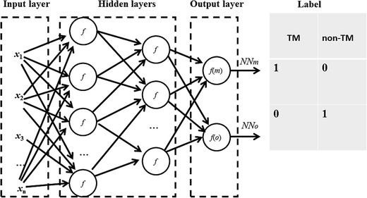
where w is the weight connecting one node of a neural network to another node, t is time step of update of weights, E is the squared error, L is the learning rate and M is the momentum. The sigmoid activation function is also used. Further description of these parameters and neural network algorithm are available at https://en.wikipedia.org/wiki/Backpropagation.28 Here, the neural network was designed with one input layer, two hidden layers, and one output layer (Fig. 1). This framework has been proven to perform well in many classification and regression problems, such as molecular dynamics simulation.33 In this framework, two nodes are set in the output layer. One node of the output layer represents the prediction probability (e.g., NNm) of a residue belonging to the TM state, while the other node (e.g., NNo) represents the probability of the residue belonging to the non-TM state. The values (1, 0) and (0, 1) are used to encode TM and non-TM residues, respectively. Again, the standard backward propagation of errors algorithm is used to optimize the weights of the neural network.32
 |
| | Fig. 1 Architecture of the neural network for TM prediction. One input layer, two hidden layers and one output layer are included in the framework. The two nodes in the output layer represent the prediction probabilities of the residues belonging to TM and non-TM states, respectively. | |
The other adopted machine learning method is random forest algorithm.34 The random forest algorithm is an ensemble algorithm that consists of many decision trees. Each decision tree gives a prediction called a vote. The final prediction is calculated by the votes in these decision trees. We used Breiman's fortran code (http://www.stat.berkeley.edu/%7Ebreiman/RandomForests) to implement the random forest framework in this work. The Intel ifort compiler was used to compile the code. The input features were the same as those used in the neural network. The methods based on the neural network and random forest algorithms were named NNME and RFME in this work. Support vector machine35 was also tested for TM prediction in this work, however, the performance is not very well (data not shown).
Propensities of TM regions for 20 amino acids
The TM propensities of 20 amino acids were calculated using a method similar to that described by Chou and Fasman36 as| |
 | (3) |
where pro(i/s) is the propensity of the ith residue in the s state (i.e., TM or non-TM states), p(i) is the frequency of the ith residue in the training sequences, and p(i/s) is the frequency of the ith residue in the s state. p(i) represents the background frequency of the ith residue and p(i/s) represents the real occurrence frequency of the ith residue in the s state. For example, there are 85![[thin space (1/6-em)]](https://www.rsc.org/images/entities/char_2009.gif) 044 Ala residues among 1
044 Ala residues among 1![[thin space (1/6-em)]](https://www.rsc.org/images/entities/char_2009.gif) 038
038![[thin space (1/6-em)]](https://www.rsc.org/images/entities/char_2009.gif) 359 residues and 45
359 residues and 45![[thin space (1/6-em)]](https://www.rsc.org/images/entities/char_2009.gif) 690 Ala residues among 457
690 Ala residues among 457![[thin space (1/6-em)]](https://www.rsc.org/images/entities/char_2009.gif) 455 TM residues. The p(i) is 85
455 TM residues. The p(i) is 85![[thin space (1/6-em)]](https://www.rsc.org/images/entities/char_2009.gif) 044/1
044/1![[thin space (1/6-em)]](https://www.rsc.org/images/entities/char_2009.gif) 038
038![[thin space (1/6-em)]](https://www.rsc.org/images/entities/char_2009.gif) 359 and the p(i/s) is 45
359 and the p(i/s) is 45![[thin space (1/6-em)]](https://www.rsc.org/images/entities/char_2009.gif) 690/457
690/457![[thin space (1/6-em)]](https://www.rsc.org/images/entities/char_2009.gif) 455. Therefore, pro(i/s) is equal to 1.219. A code implementing this algorithm by our group is publicly available at http://genomics.fzu.edu.cn/nnme/propensity/. More details of the propensity calculation are provided in ESI 1.†
455. Therefore, pro(i/s) is equal to 1.219. A code implementing this algorithm by our group is publicly available at http://genomics.fzu.edu.cn/nnme/propensity/. More details of the propensity calculation are provided in ESI 1.†
TM prediction based on the hydropathy profile
Hydropathy information was used as an alternative method of TM prediction in this work. Here, Kyte–Doolittle37 was used to calculate the hydropathy profile of amino acid sequences. Briefly, a sliding window containing 2n + 1 adjacent residues (i.e., window size equal to 2n + 1) of the fragment sequence centered at the target residue is excised from the protein sequence. Next, the average hydropathy over the segment is calculated and used as the prediction score. For residues located close to the termini, the lengths of the fragments are less than the pre-defined window size and thus shorter fragments are used to calculate the average hydropathy score (i.e., prediction score by the hydropathy predictor). We also tested the Chothia measure38 in this work. The optimal window sizes of both measures were determined by the area under the ROC39 curve in the training dataset and were set to 15.
Performance assessment measure
When the benchmark was performed on the datasets for TM region prediction, the overall performance of the heterogeneous methods was evaluated with respect to the following parameters: accuracy (Ac), sensitivity (Sn), specificity (Sp), error rate (Er), false positive rate (Fpr), false negative rate (Fnr) and Matthew correlation coefficient (Mcc). The measures of Er, Fpr and Fnr were calculated to estimate the prediction performance by various numbers of trees. The TM and non-TM residues were defined as positive and negative samples in this work. These measures were calculated as follows| |
 | (4) |
| |
 | (5) |
| |
 | (6) |
| |
 | (7) |
where tp, tn, fp and fn represent the numbers of true-positives, true-negatives, false-positives and false-negatives, respectively. It should be mentioned here that the metrics used here are suitable for single-label systems (i.e., two-class classification problems), whereas metrics for multi-label systems should refer to the some relating references.40,41 According to ref. 24, 42 and 43, eqn (4)–(7) can be rewritten as| |
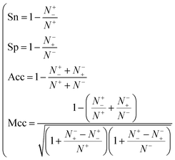 | (8) |
where N+ and N− represent the numbers of positive and negative samples. Meanwhile, N+− is the number of false-negatives and N−+ is the number of false-positives. Different expression patterns can likely deepen our understanding of the significance of these measures. Random forest is an out-of-bag algorithm. Therefore, Er, Fpr and Fnr are used to assess the prediction of random forests consisting of different numbers of trees.| |
 | (9) |
| |
 | (10) |
| |
 | (11) |
It should be mentioned that not all predictions of TM/non-TM regions are reliable. Therefore, we also used an equation similar to that proposed by Rost and Sander44 to estimate the reliable index (RI) of the prediction for each residue as follows
| | |
ReliableIndex = INT(10(|OUTm − OUTo|))
| (12) |
where OUT
m is the prediction score for a residue to be TM and OUT
o is the prediction score for the residue to be non-TM. The higher the RI score is, the more reliable prediction for the residue is. In the neural network, OUT
m and OUT
o are scores calculated in the two output nodes. Similarly, OUT
m and OUT
o are prediction probabilities for TM and non-TM in the random forest method. The reliable indexes for neural network and random forest methods were named NNRI and RFRI in this work. In addition, we simply used the ROC
45 curve, which plots the true positive rate against the false positive rate, to assess the performance for membrane protein identification. The measure of the identification of a membrane protein is simply calculated as
| |
 | (13) |
where
n is the number of residues of a target protein, and OUT
m[
i] and OUT
o[
i] are calculated for residue
i using
eqn (11).
Results and discussion
Machine learning-based predictors
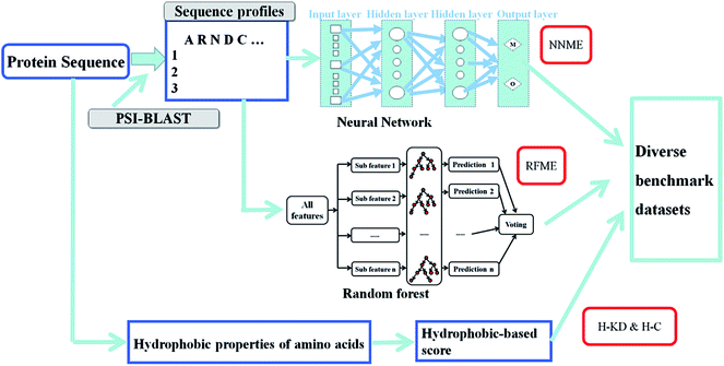
Here, we relied on both TRAIN4241 and TEST3450 datasets to assess the performance of various predictors. Fig. 2 shows the framework of the benchmark procedure. We performed the cross-validation scheme to test the predictors on the TRAIN4241 dataset. N-fold cross-validation, sub-sampling test, and independent dataset test are widely used to test the performance of prediction methods.46–48 Jackknife test is a specific type of cross-validation method.49,50 In the jackknife test, each sample is in turn singled out as an independent test and the model was constructed using the remaining samples. Considering the size of the training dataset, we used a 30-fold cross-validation procedure to benchmark our method. The TRAIN4241 dataset was divided into 30 roughly equal subsets. One subset was then used as a test dataset and the remaining 29 subsets were combined to train one or several models for TM prediction. This procedure was repeated 30 times until all subsets were tested (i.e., each subset was used as the test dataset one time). Briefly, each subset was benchmarked by the model trained by other 29 subsets to avoid over fitting. Meanwhile, random forest is an out-of-bag algorithm and the error rates of trainings were also estimated. The error rate of non-membrane regions (e.g., false-negative rate) and error rate of TM regions (e.g., false-positive rate) of the random forest method consisting of different numbers of trees were estimated. Both the neural network and random forest models were strictly benchmarked in the cross-validation procedure. In this procedure, the neural network model was intensively trained and generated the values of Ac = 0.861 and Mcc = 0.716 on the TRAIN4241 dataset (Table 1). Additionally, an independent test scheme was further used to validate the performance of the predictors. In this scheme, TEST3450 dataset was used to assess the performance of the trained models, which were intensively optimized on the complete the TRAIN4241 dataset. Further, the NNME method achieved values of Ac = 0.951 and Mcc = 0.734 on the TEST3450 dataset. Similarly, the random forest-based predictor generated values of Ac = 0.849 and Mcc = 0.691 on the TRAIN4241 in the cross-validation procedure. And the random forest-based predictor generated values of Ac = 0.944 and Mcc = 0.691 on the TEST3450 when using the models trained on the TRAIN4241. The different performance of a predictor (e.g., NNME) on the training and test datasets probably can likely be attributed to two reasons. First, the model used to benchmark the performance of the TEST3450 dataset is larger than that constructed in the cross-validation procedure. Second, the rates of positive and negative samples on the training and test dataset are differed. The rate of a dataset usually affects the prediction results. Meanwhile, it is reasonable that a predictor generates different values of accuracy on different datasets. These two predictors were constructed using features of PSSM, PSFM, secondary structure and solvent accessibility. Furthermore, we designed two variants of NNME methods (i.e., NNME-I and NNME-II) by removing the secondary structure (SS) and/or solvent accessibility (SA) information. As shown in Table 1, there was only a slight decrease in accuracy. Features of SS, SA and PSSM profiles (i.e., evolutionary information) may reflect the similar aspects of proteins and, to a limited extent, can be complementary. Moreover, the prediction accuracy obtained by using only sequence evolutionary profiles was very high, as the Mcc value of prediction was only approximately 1.5% lower when the SS and SA features were removed from the trained model. Similar results were obtained for RFME-I and RFME-II predictors. These results suggest that protein PSSM and PSFM features contribute most to the final model. Meanwhile, solvent accessibility (SA) is a one-dimensional feature, and the Pcc correlation between it and TM propensity is 0.446, suggesting only a slight correlation between SA and TM. Furthermore, most TM regions locate in α-helix and β-strand regions. Therefore, SS information is useful. However, SS information is also predicted by PSSM and PSFM features, and its contribution to the final performance may overlap with PSSM and PSFM features to some extent. It should be mentioned that the parameters of the developed methods were optimized by using a simple grid search. The optimal performance of NNME and RFME methods was obtained when the window size was set at 19. The node numbers in two hidden layers of the NNME method were 150 and 150. The number of variables to split on each node of the RFME method was set at 3. Additionally, the number of trees of the RFME method was optimized at a value of 1000. When more trees were added to the RFME method, improved performance was not obtained.
 |
| | Fig. 2 Flowchart of the benchmark procedure for membrane protein prediction. | |
Table 1 TM prediction of various methods
| Method |
Ac |
Sn |
Sp |
Mcc |
| These features were trained using the neural network (NN) and random forest (RF) algorithms, respectively. NNME-I and NNME-II are two variants of the NNME method. NNME-I and NNME-II were trained by removing secondary structure (SS) and/or solvent accessibility (SA) information from the input features. Similarly, RFME-I and RFME-II are also two variants of the RFME method, which were generated by removing the corresponding features. H-KD and H-C indicate hydropathy-based predictors by using Kyte–Doolittle and Chothia measures, respectively. The window sizes of NNME and RFME were optimized at the size of 19. |
| Benchmark results of the TRAIN4241 dataset |
| HMMTOP |
0.871 |
0.847 |
0.889 |
0.737 |
| TMHMM |
0.885 |
0.862 |
0.903 |
0.766 |
| Memsat |
0.832 |
0.826 |
0.837 |
0.659 |
| Phobius |
0.874 |
0.853 |
0.889 |
0.742 |
| MemBrain |
0.838 |
0.824 |
0.848 |
0.669 |
| (PSSM + PSFM)NNME-Ia |
0.855 |
0.848 |
9.860 |
0.705 |
| (PSSM + PSFM + SS)NNME-IIa |
0.857 |
0.847 |
0.866 |
0.710 |
| (PSSM + PSFM + SS + SA)NNMEa |
0.861 |
0.848 |
0.871 |
0.716 |
| (PSSM + PSFM)RFME-Ia |
0.845 |
0.806 |
0.873 |
0.681 |
| (PSSM + PSFM + SS)RFME-IIa |
0.845 |
0.828 |
0.857 |
0.683 |
| (PSSM + PSFM + SS + SA)RFa |
0.849 |
0.808 |
0.879 |
0.691 |
| Kyte-DoolittleH-KD |
0.810 |
0.806 |
0.813 |
0.615 |
| ChothiaH-C |
0.781 |
0.721 |
0.826 |
0.550 |
![[thin space (1/6-em)]](https://www.rsc.org/images/entities/char_2009.gif) |
| Benchmark results of the TEST3450 dataset |
| HMMTOP |
0.872 |
0.848 |
0.889 |
0.738 |
| TMHMM |
0.846 |
0.817 |
0.871 |
0.689 |
| Memsat |
0.944 |
0.721 |
0.968 |
0.684 |
| Phobius |
0.836 |
0.829 |
0.843 |
0.671 |
| MemBrain |
0.946 |
0.797 |
0.962 |
0.715 |
| (PSSM + PSFM)NNME-Ia |
0.951 |
0.784 |
0.969 |
0.734 |
| (PSSM + PSFM + SS)NNME-IIa |
0.951 |
0.783 |
0.969 |
0.731 |
| (PSSM + PSFM + SS + SA)NNMEa |
0.953 |
0.777 |
0.972 |
0.737 |
| (PSSM + PSFM)RFME-Ia |
0.941 |
0.709 |
0.966 |
0.671 |
| (PSSM + PSFM + SS)RFME-IIa |
0.942 |
0.667 |
0.975 |
0.678 |
| (PSSM + PSFM + SS + SA)RFa |
0.944 |
0.741 |
0.966 |
0.691 |
| Kyte–DoolittleH-KDa |
0.862 |
0.810 |
0.867 |
0.503 |
| ChothiaH-Ca |
0.848 |
0.718 |
0.862 |
0.435 |
![[thin space (1/6-em)]](https://www.rsc.org/images/entities/char_2009.gif) |
| Benchmark results for combined methods of the TEST3450 dataset |
| NN + RF |
0.950 |
0.785 |
0.968 |
0.729 |
| NN + hydropathy |
0.953 |
0.656 |
0.984 |
0.710 |
| NN + RF + hydropathy |
0.953 |
0.685 |
0.982 |
0.721 |
A hydropathy-based predictor
In addition to profile-based predictors, simple hydropathy-based methods were also employed for TM region prediction. Kyte–Doolittle and Chothia are two widely used hydropathy measures. The Pearson correlation coefficient (Pcc) between these two measures is 0.889 (http://genomics.fzu.edu.cn/nnme/KdcPcc.pl). Therefore, it is important to compare the TM prediction performance of the new model described herein with these two measures. The average hydropathy of a segment sequence is used to predict whether the center amino acid of the segment is TM or not. To optimize the segment size of the hydropathy-based predictor, we used the area under ROC curve (i.e., AUC score) as a main measure. The distribution of AUC scores with various window sizes is shown in Table 2. Both hydropathy-based methods of Kyte–Doolittle (H-KD predictor) and Chothia (H-C predictor) achieved optimal performance at the size of 15, and generated AUC scores of 0.898 and 0.868, respectively, on the TRAIN4241 dataset when the window size was set at this value. Additionally, H-KD and H-C predictors generated Mcc values of 0.550 and 0.435, respectively, on the TEST3450 dataset. However, the prediction accuracy was not improved when combining these two measures.
Table 2 Distribution of AUC values by H-predictors for different window sizes
| Size |
5 |
7 |
9 |
11 |
13 |
15 |
17 |
19 |
21 |
| Kyte–Doolittle |
0.851 |
0.873 |
0.887 |
0.894 |
0.897 |
0.898 |
0.896 |
0.892 |
0.887 |
| Chothia |
0.821 |
0.843 |
0.856 |
0.863 |
0.867 |
0.868 |
0.866 |
0.863 |
0.857 |
Combining different predictors
We next tested a hybrid predictor by combining the sequence profile and hydropathy-based methods with a linear equation (i.e., ScoreNNME + αScoreRFME + βScoreH). Here, ScoreNNME and ScoreRFME represent the profile-based prediction scores by the neural network and random forest-based methods, respectively. ScoreH is the prediction score generated by the hydropathy-based predictor. α and β are parameters that were optimized on the training dataset to balance different terms. In fact, sequence profile and hydrophobicity are likely complementary information. We therefore attempted to combine them to increase the prediction accuracy. A linear combination of these two methods was intensively tested in this work. However, improved accuracy was not obtained. We also directly added two predictors (i.e., NNME + H-KT and NNME + RFME), which resulted in even lower Mcc values compared to the single NNME predictor. This observation is probably because the same input features were used by the neural network and random forest-based predictors. Therefore, the complementary information between these two predictors is highly limited. (See ESI 2† for details). Meanwhile, the accuracy of the neural network-based method is already very high, and it is therefore difficult to improve it simply by using hydropathy-based information.
Propensities of 20 amino acids in TM and non-TM regions
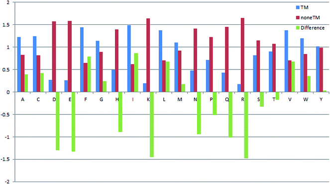
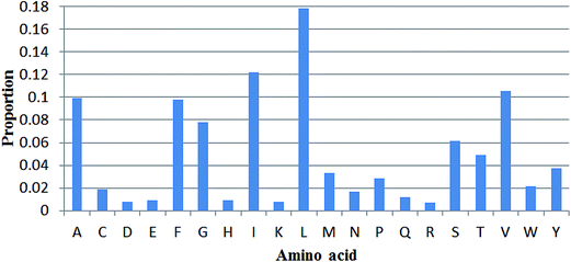
The propensities of 20 amino acids located in TM and non-TM regions are shown in Fig. 3, in which the different amino acid propensities for TM and non-TM are also given. The different values were calculated by subtracting the non-TM values from the corresponding TM values. Residues with positive scores suggest that those residues are located in the TM region and vice versa. As shown in Table 3, A(Ala), C(Cys), F(Phe), G(Gly), I(Ile), L(Leu), V(Val), and W(Trp) are more preferred in TM regions, while R(Arg), D(Asp), E(Glu), H(His), K(Lys), N(Asn), P(Pro), Q(Gln), S(Ser), and T(Thr) are more prevalent in non-TM regions. Meanwhile, M(Met) and Y(Tyr) only show subtle differences in the two regions. Interestingly, Gromiha and co-workers also developed a similar parameter for α-helix region location. The Pcc value between these two sets of parameters is 0.737, suggesting a correlation between the two sets of measures. Meanwhile, the proportion of 20 amino acids located in TM regions was also analyzed (Fig. 4). As shown in Fig. 4, R(Arg) has the least possibility while L(Leu) has the highest possibility of being located in a TM region.
 |
| | Fig. 3 Propensities of 20 amino acids located in TM and non-TM regions. | |
Table 3 Propensities of 20 amino acids located in transmembrane/non-transmembrane regions
| Amino acid |
TM |
non-TM |
Difference |
| A |
1.219 |
0.827 |
0.406 |
| C |
1.238 |
0.813 |
−0.336 |
| D |
0.271 |
1.574 |
−1.312 |
| E |
0.259 |
1.583 |
−0.392 |
| F |
1.443 |
0.651 |
0.550 |
| G |
1.136 |
0.893 |
−0.258 |
| H |
0.500 |
1.394 |
−0.119 |
| I |
1.484 |
0.619 |
−0.154 |
| K |
0.190 |
1.638 |
−0.513 |
| L |
1.377 |
0.703 |
0.456 |
| M |
1.100 |
0.921 |
−0.314 |
| N |
0.474 |
1.414 |
−0.752 |
| P |
0.713 |
1.226 |
−0.736 |
| Q |
0.430 |
1.449 |
−1.220 |
| R |
0.174 |
1.650 |
−0.971 |
| S |
0.816 |
1.145 |
−0.260 |
| T |
0.903 |
1.076 |
0.202 |
| V |
1.379 |
0.701 |
0.536 |
| W |
1.199 |
0.843 |
0.214 |
| Y |
1.019 |
0.985 |
1.019 |
 |
| | Fig. 4 Proportions of 20 amino acids located in TM regions. | |
Significance of prediction scores
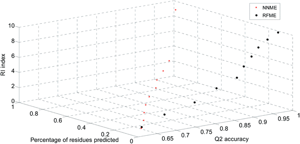
The significance of prediction scores of the developed predictors was also estimated in this work. The reliable levels of prediction scores of NNME and RFME predictors were calculated based on the TRAIN4241 dataset (Fig. 5). For the NNME predictor, there are two nodes in the output layer. The difference in prediction scores by these two nodes (i.e., reliable index defined in eqn (11)) can be used to estimate the reliable level of a prediction. Similar reliable parameters should refer to previous reports.51,52 In general, the larger the reliable index, the more significant the prediction. In our benchmark results, NNRI generated a prediction at the 99% and 95% confident levels when its values were greater than 0.90 and 0.45 (Fig. 5). Similarly, the random forest-based predictor generated a prediction at the 99% and 95% confident levels when the RFRI values were greater than 0.50 and 0.30. The number of trees is an important parameter that affects the prediction score of the random forest method. Therefore, the average errors of RFME method by combining different numbers trees were estimated (Table 4).
 |
| | Fig. 5 Reliable indices for neural network- and random forest-based predictors. | |
Table 4 Average error of the random forest-based method on 30 subsets of the TRAIN4241 dataset using the out-of-bag method
| # of trees |
Er |
Fnr |
Fpr |
| 10 |
24.33 |
15.55 |
36.72 |
| 100 |
16.32 |
12.63 |
21.84 |
| 300 |
15.43 |
12.19 |
20.34 |
| 500 |
15.25 |
12.12 |
20.02 |
| 700 |
15.18 |
12.11 |
19.88 |
| 1000 |
15.14 |
12.09 |
19.79 |
Comparison with other state-of-the-art methods
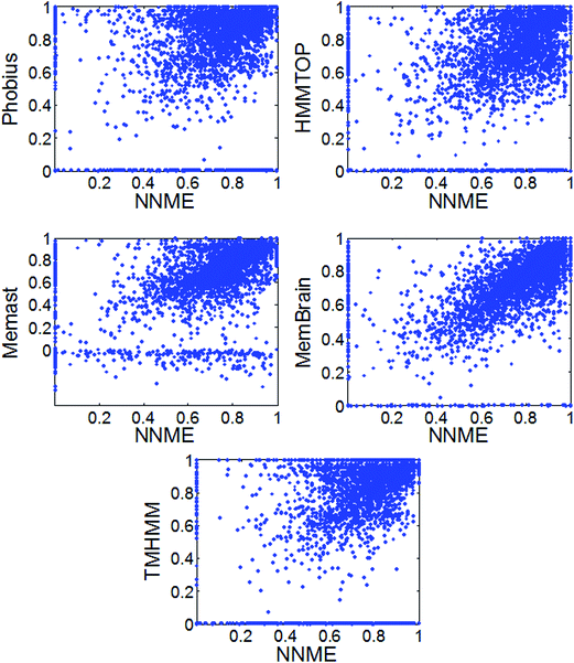
Here, the state-of-the-art methods, TMHMM,18 HMMTOP,19 Memsat,53 Phobius54 and MemBrain20 were benchmarked and compared. Local programs of TMHMM, HMMTOP, Memsat, Phobius were downloaded and sequences were directly fed into them. With respect to MemBrain, we wrote a simple Perl script and automatically submit sequences to its web server (http://www.csbio.sjtu.edu.cn/bioinf/MemBrain). As shown in Table 1, the Mcc values generated by these methods were in the range of 0.635 to 0.742 on the TEST3450 dataset. The NNME method generated an Mcc value of 0.691 on the TEST3450 dataset. Similar results were obtained on the TRAIN4241 dataset. Some of these tested proteins are likely similar to those used to train these methods. Meanwhile, the Mcc values for 3450 proteins of the TEST3450 dataset by different methods were also shown in Fig. 6. As can be seen from the figure, NNME is complementary to Phobius, TMHMM and HMMTOP (e.g., many points distribute in the upper and lower triangles of figures). But the complementarity between NNME and RFME is low (ESI 2†), which is likely because the same input features were used by these two methods. The Uniprot website describes how TM domains are annotated automatically by their sequence annotation module using TMHMM.18 Therefore, it is not surprising to learn that the Mcc value generated by TMHMM was very high. In fact, the methods tested are very suitable for genome-wide prediction. For example, a simple script can be written to submit thousands of sequences to the MemBrain20 server, which will generate highly accurate results in a very short time (approximately several seconds for a protein).
 |
| | Fig. 6 Comparison of different TM prediction methods on the TEST3450 dataset. | |
Identification of membrane proteins from large datasets
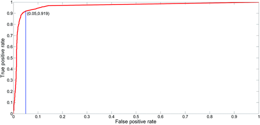
The proposed NNME predictor is very reliable for TM prediction. Therefore, it is also very interesting and useful to investigate its performance of distinguishing globular and membrane proteins. Therefore, we tested the IdenM measure, which is defined in eqn (12) to distinguish the GLO4473 and TEST3450 datasets. Proteins in the GLO4473 dataset were non-membrane proteins. The complete TEST3450 dataset, which consists of 3450 membrane proteins, was directly used. The identification model was trained on the TRAIN4241 dataset. Discrimination performance of the trained predictor was assessed by discriminating membrane proteins from non-membrane proteins. The performance of the NNME method on the identification of membrane proteins was clearly shown in Fig. 7. As can be seen from the figure, the NNME method correctly identified 91.93% of membrane proteins at a false-positive rate of 5%. To reduce the false-positives, advanced users may choose threshold values with a higher confidence level, but the number of true-positives will be reduced accordingly.
 |
| | Fig. 7 ROC curve for the identification of membrane proteins using the NNME method. | |
Sequence-based versus structure-based benchmarks
Some proteins in the Uniprot database are structurally unknown. However, structurally known proteins can provide more accurate feature information. Therefore, it is very interesting to train or benchmark these structurally known proteins. Here, all sequences in both TRAIN4241 and TEST3450 datasets were submitted to the ID mapping tool on the Uniprot website. Among them, 91 out of TRAIN4241 sequences and 213 out of TEST3450 sequences can be successfully mapped to structurally known proteins. More importantly, all of these entries were reviewed by experts (i.e., contain reviewed keywords in the annotation tables). Finally, we obtained 304 proteins that proteins can be regarded as a more reliable dataset. The entries of these 304 proteins are also publicly available at http://genomics.fzu.edu.cn/nnme/datasets. The prediction results by different methods for these 304 proteins (i.e., STR304 dataset) were shown in Table 5. It should be noted that the prediction results for these proteins of the NNME method were generated in the cross-validation procedure so that over-fitting problem can be avoided. As can be seen, slightly different results were generated on the STR304 dataset. But it is not very surprise to see it according to the fact that the size of the STR304 is much smaller than the TRAIN4241 and TEST3450 datasets. Anyway, methods tested (e.g., MemBrain) herein can generate a prediction in a very short time and are very suitable for genome-wide applications.
Table 5 TM prediction by various methods on the STR304 dataset
| Method |
Ac |
Sn |
Sp |
Mcc |
| Benchmark results of the STR309 dataset |
| HMMTOP |
0.939 |
0.715 |
0.970 |
0.707 |
| TMHMM |
0.951 |
0.737 |
0.980 |
0.759 |
| Memsat |
0.939 |
0.723 |
0.969 |
0.710 |
| Phobius |
0.954 |
0.751 |
0.982 |
0.775 |
| MemBrain |
0.936 |
0.736 |
0.963 |
0.700 |
| (PSSM + PSFM + SS + SA)NNME |
0.963 |
0.742 |
0.979 |
0.719 |
A case study of TM prediction
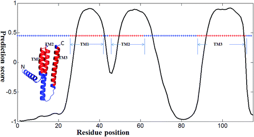
We developed several methods for TM prediction (e.g., NNME and RFME). Among them, NNME is the most reliable and it is useful if a case study for this method is clearly shown. A real application of the NNME method for TM prediction was exemplified in Fig. 8. The example is a membrane protein with a sequence length of 150 amino acids (PDB entry: 3ZE5A55). Based on the annotation from the Uniprot database (access name: P0ABN1), the membrane protein, which acts as a diacylglycerol kinase, contains three helical TM regions (TM1 spans residues 27–42, TM2 spans residues 46–62 and TM3 spans residues 89–112). The x-axis of the figure shows the sequence position and the y-axis shows the prediction score. As shown in Fig. 8, the TM regions of the protein structure are colored in red. Meanwhile, an asterisk line representing the sequence state (i.e., TM regions are colored in red and non-TM regions are colored in blue) is also embedded in the figure. The sequence of the 3ZE5A protein was directly tested using the NNME method. As can be seen, positions of amino acids 29–42, 50–65 and 93–110 were predicted as TM regions. The prediction result is reliable (Ac = 0.900), and the prediction accuracy is similar to that obtained on the TEST3450 dataset. The 3D structure of the protein was visualized using the PyMOL56 program. It should be noted that this case was used to show a realistic application of the NNME method rather than provide a performance comparison between the different methods. The prediction score and other relative results of the case are publicly available at http://genomics.fzu.edu.cn/nnme/case/.
 |
| | Fig. 8 A case study of the NNME method. The tested protein is 3ZE5A, where “3Z5E” is the Protein Data Bank entry and “A” is the chain identifier. In the 3D structure, three transmembrane regions are shown in red (i.e., TM1, TM2 and TM3). The x-axis shows the residue position of the protein and the y-axis shows the prediction value generated by the NNME method. An asterisk line indicating residue state is also shown. Red asterisks represent TM residues, while blue asterisks indicate non-TM residues. The asterisk line (i.e., 0.45) is set at the 95% confidence cutoff of NNME to predict whether a residue is TM or not. | |
Conclusions
Taken together, several membrane predictors were developed and strictly benchmarked using two non-redundant and diverse datasets in this work. The neural network-based predictor, which was trained on large-scale datasets using sequence evolutionary profiles, secondary structure and solvent accessibility as features, can significantly complement and guide experimental efforts. Furthermore, a stand-alone program implementing the NNME method was constructed, which can be directly run on local computers for high-throughput sequences. The predictor can also be used to identify membrane proteins from genome-wide sequences. The performance of our predictor mostly depends on sequence evolutionary information. If sequence evolutionary information is polluted, the accuracy of the prediction results may decrease, which is one of the pitfalls of our method. The developed method should become an easy-to-use and accurate tool in the scientific community. Although the proposed method is based on computation algorithms, we hope its development will strengthen our knowledge of the molecular mechanisms and functionalities of membrane proteins.
Acknowledgements
This work was supported by National Natural Science Foundation of China (31500673 and 31571300), Start-Up Fund of Fuzhou University (510046), and Science Development Foundation of Fuzhou University (2013-XY-17).
References
- M. S. Almen, K. J. Nordstrom, R. Fredriksson and H. B. Schioth, BMC Biol., 2009, 7, 50 CrossRef PubMed.
- M. Wistrand, L. Kall and E. L. Sonnhammer, Protein Sci., 2006, 15, 509–521 CrossRef CAS PubMed.
- K. C. Chou and H. B. Shen, PLoS One, 2010, 5, e9931 Search PubMed.
- X. Xiao, J. L. Min, P. Wang and K. C. Chou, PLoS One, 2013, 8, e72234 CAS.
- P. Marani, S. Wagner, L. Baars, P. Genevaux, J. W. de Gier, I. Nilsson, R. Casadio and G. von Heijne, Protein Sci., 2006, 15, 884–889 CrossRef CAS PubMed.
- J. P. Overington, B. Al-Lazikani and A. L. Hopkins, Nat. Rev. Drug Discovery, 2006, 5, 993–996 CrossRef CAS PubMed.
- M. Stamm, R. Staritzbichler, K. Khafizov and L. R. Forrest, Nucleic Acids Res., 2014, 42, W246–W251 CrossRef CAS PubMed.
- K. C. Chou, J. Proteome Res., 2005, 4, 1413–1418 CrossRef CAS PubMed.
- K. C. Chou and H. B. Shen, Nat. Protoc., 2008, 3, 153–162 CrossRef CAS PubMed.
- M. Remmert, D. Linke, A. N. Lupas and J. Soding, Nucleic Acids Res., 2009, 37, W446–W451 CrossRef CAS PubMed.
- C. Dong, K. Beis, J. Nesper, A. L. Brunkan-Lamontagne, B. R. Clarke, C. Whitfield and J. H. Naismith, Nature, 2006, 444, 226–229 CrossRef CAS PubMed.
- N. Sapay, Y. Guermeur and G. Deleage, BMC Bioinf., 2006, 7, 255 CrossRef PubMed.
- J. E. Johnson and R. B. Cornell, Mol. Membr. Biol., 1999, 16, 217–235 CrossRef CAS PubMed.
- V. Yarov-Yarovoy, J. Schonbrun and D. Baker, Proteins, 2006, 62, 1010–1025 CrossRef CAS PubMed.
- P. Argos, J. K. Rao and P. A. Hargrave, Eur. J. Biochem., 1982, 128, 565–575 CrossRef CAS PubMed.
- B. Rost, P. Fariselli and R. Casadio, Protein Sci., 1996, 5, 1704–1718 CrossRef CAS PubMed.
- L. Rabiner, Proc. IEEE, 1989, 77, 257–286 CrossRef.
- A. Krogh, B. Larsson, G. von Heijne and E. L. Sonnhammer, J. Mol. Biol., 2001, 305, 567–580 CrossRef CAS PubMed.
- G. E. Tusnady and I. Simon, Bioinformatics, 2001, 17, 849–850 CrossRef CAS PubMed.
- H. Shen and J. J. Chou, PLoS One, 2008, 3, e2399 Search PubMed.
- D. T. Jones, W. R. Taylor and J. M. Thornton, Biochemistry, 1994, 33, 3038–3049 CrossRef CAS PubMed.
- G. von Heijne, J. Mol. Biol., 1992, 225, 487–494 CrossRef CAS PubMed.
- K. C. Chou, J. Theor. Biol., 2011, 273, 236–247 CrossRef CAS PubMed.
- W. Chen, P. M. Feng, H. Lin and K. C. Chou, Nucleic Acids Res., 2013, 41, e68 CrossRef CAS PubMed.
- Y. Xu, X. J. Shao, L. Y. Wu, N. Y. Deng and K. C. Chou, PeerJ, 2013, 1, e171 Search PubMed.
- M. van Geest and J. S. Lolkema, Microbiol. Mol. Biol. Rev., 2000, 64, 13–33 CrossRef CAS PubMed.
- E. Boutet, D. Lieberherr, M. Tognolli, M. Schneider and A. Bairoch, Methods Mol. Biol., 2007, 406, 89–112 CAS.
- S. F. Altschul, W. Gish, W. Miller, E. W. Myers and D. J. Lipman, J. Mol. Biol., 1990, 215, 403–410 CrossRef CAS PubMed.
- N. K. Fox, S. E. Brenner and J. M. Chandonia, Nucleic Acids Res., 2014, 42, D304–D309 CrossRef CAS PubMed.
- R. Yan, X. Wang, L. Huang, F. Yan, X. Xue and W. Cai, Sci. Rep., 2015, 5, 11586 CrossRef CAS PubMed.
- J. Heaton, Introduction to Neural Networks with Java, Heaton Research, 2008, pp. 1–429 Search PubMed.
- D. E. Rumelhart, G. E. Hinton and R. J. Williams, Nature, 1986, 323, 533–536 CrossRef.
- F. Häse, S. Valleau, E. Pyzerknapp and A. Aspuruguzik, Chem. Sci., 2016, 7, 5139 RSC.
- B. Leo, Machine Learning, Kluwer Academic Publishers, 2001, vol. 45, pp. 5–32 Search PubMed.
- T. Joachims, Advances in Kernel Methods, MIT Press, 1999, pp. 14–28 Search PubMed.
- P. Y. Chou and G. D. Fasman, Adv. Enzymol. Relat. Areas Mol. Biol., 1978, 47, 45–148 CAS.
- J. Kyte and R. F. Doolittle, J. Mol. Biol., 1982, 157, 105–132 CrossRef CAS PubMed.
- C. Chothia, J. Mol. Biol., 1976, 105, 1–12 CrossRef CAS PubMed.
- K. Soreide, J. Clin. Pathol., 2009, 62, 1–5 CrossRef PubMed.
- K. C. Chou, Z. C. Wu and X. Xiao, PLoS One, 2011, 6, e18258 CAS.
- K. C. Chou, Z. C. Wu and X. Xiao, Mol. BioSyst., 2012, 8, 629–641 RSC.
- H. Lin, E. Z. Deng, H. Ding, W. Chen and K. C. Chou, Nucleic Acids Res., 2014, 42, 12961–12972 CrossRef CAS PubMed.
- S. H. Guo, E. Z. Deng, L. Q. Xu, H. Ding, H. Lin, W. Chen and K. C. Chou, Bioinformatics, 2014, 30, 1522–1529 CrossRef CAS PubMed.
- B. Rost and C. Sander, J. Mol. Biol., 1993, 232, 584–599 CrossRef CAS PubMed.
- J. A. Swets, Signal detection theory and ROC analysis in psychology and diagnostics: Collected papers, Psychology Press, 2014 Search PubMed.
- C. J. Zhang, H. Tang, W. C. Li, H. Lin, W. Chen and K. C. Chou, Oncotarget, 2016, 7, 69783–69793 Search PubMed.
- H. Yang, H. Tang, X. X. Chen, C. J. Zhang, P. P. Zhu, H. Ding, W. Chen and H. Lin, BioMed Res. Int., 2016, 2016, 5413903 Search PubMed.
- H. Ding, L. Luo and H. Lin, Protein Pept. Lett., 2009, 16, 351–355 CrossRef CAS PubMed.
- K. C. Chou and C. T. Zhang, Crit. Rev. Biochem. Mol. Biol., 1995, 30, 275–349 CrossRef CAS PubMed.
- H. Ding, W. Yang, H. Tang, P. M. Feng, J. Huang, W. Chen and H. Lin, Virol. Sin., 2016, 31, 350–352 CrossRef PubMed.
- D. T. Jones, J. Mol. Biol., 1999, 292, 195–202 CrossRef CAS PubMed.
- R. Yan, X. Wang, L. Huang, J. Lin, W. Cai and Z. Zhang, Mol. BioSyst., 2014, 2495–2504, 10.1039/c4mb00272e.
- D. T. Jones, FEBS Lett., 1998, 423, 281–285 CrossRef CAS PubMed.
- L. Kall, A. Krogh and E. L. Sonnhammer, J. Mol. Biol., 2004, 338, 1027–1036 CrossRef CAS PubMed.
- D. Li, J. A. Lyons, V. E. Pye, L. Vogeley, D. Aragao, C. P. Kenyon, S. T. Shah, C. Doherty, M. Aherne and M. Caffrey, Nature, 2013, 497, 521–524 CrossRef CAS PubMed.
- V. r. p. The PyMOL Molecular Graphics System, Schrödinger, LLC Search PubMed.
Footnote |
| † Electronic supplementary information (ESI) available. See DOI: 10.1039/c7ra03883f |
|
| This journal is © The Royal Society of Chemistry 2017 |
Click here to see how this site uses Cookies. View our privacy policy here.  Open Access Article
 *a,
Xiaofeng Wangb,
Lanqing Huanga,
Yarong Tiana and
Weiwen Caia


![[thin space (1/6-em)]](https://www.rsc.org/images/entities/char_2009.gif) 044 Ala residues among 1
044 Ala residues among 1![[thin space (1/6-em)]](https://www.rsc.org/images/entities/char_2009.gif) 038
038![[thin space (1/6-em)]](https://www.rsc.org/images/entities/char_2009.gif) 359 residues and 45
359 residues and 45![[thin space (1/6-em)]](https://www.rsc.org/images/entities/char_2009.gif) 690 Ala residues among 457
690 Ala residues among 457![[thin space (1/6-em)]](https://www.rsc.org/images/entities/char_2009.gif) 455 TM residues. The p(i) is 85
455 TM residues. The p(i) is 85![[thin space (1/6-em)]](https://www.rsc.org/images/entities/char_2009.gif) 044/1
044/1![[thin space (1/6-em)]](https://www.rsc.org/images/entities/char_2009.gif) 038
038![[thin space (1/6-em)]](https://www.rsc.org/images/entities/char_2009.gif) 359 and the p(i/s) is 45
359 and the p(i/s) is 45![[thin space (1/6-em)]](https://www.rsc.org/images/entities/char_2009.gif) 690/457
690/457![[thin space (1/6-em)]](https://www.rsc.org/images/entities/char_2009.gif) 455. Therefore, pro(i/s) is equal to 1.219. A code implementing this algorithm by our group is publicly available at http://genomics.fzu.edu.cn/nnme/propensity/. More details of the propensity calculation are provided in ESI 1.†
455. Therefore, pro(i/s) is equal to 1.219. A code implementing this algorithm by our group is publicly available at http://genomics.fzu.edu.cn/nnme/propensity/. More details of the propensity calculation are provided in ESI 1.†


![[thin space (1/6-em)]](https://www.rsc.org/images/entities/char_2009.gif)
![[thin space (1/6-em)]](https://www.rsc.org/images/entities/char_2009.gif)
