Stable sandwich structures of two-dimensional iron borides FeB_x alloy: a first-principles calculation

Abstract

Due to the complexity of the interaction between boron and 3d transition metals, stable two-dimensional (2D) iron borides FeB_x compounds have attracted tremendous attention in recent years. Combining the evolutionary algorithm with first-principles calculations, we have systematically investigated the structural stabilities and electronic properties of 2D iron borides FeB_x (x = 2–10) alloys. It is found that the multilayer iron borides FeB_x (x = 4, 6, 8, 10) are wide-band-gap semiconductors, which are more stable than the corresponding monolayers. Furthermore, the electronic and optical properties of these semiconductors may be modulated by biaxial strains, indicating their potential application for advanced blue/UV light optoelectronic devices.

---

1. Introduction

Due to their electron deficiency, boron (B) nanostructures have attracted both theoretical and experimental attention in the past decades.^1–3 Experimental observations have shown a striking evolution of B clusters as their size increases, including planar/quasi-planar structures with tetragonal/pentagonal/hexagonal defects and hollow cages.^4–12 Meanwhile, the configurations of boron clusters can be further modulated by introducing the transition metal (TM) atoms. Various planar hyper-coordinate species of TM@B_n (n = 7–10) with TM atom at the center of the boron wheel have been confirmed theoretically and experimentally, such as [FeB₈²⁻], [CoB₈⁻], [FeB₉⁻],^13,14 M@B₉⁻ (M = Ru, Rh, Ir),^14,15 and M@B₁₀⁻ (M = Ta, Nb).¹⁶ Recent progress showed that [CoB₁₆⁻]¹⁷ and [MnB₁₆⁻]¹⁸ are boron molecular drums with 16 nearest neighbor B atoms, while [CoB₁₈⁻]¹⁹ and [RhB₁₈⁻]²⁰ can be considered as the planar motifs for the metallo-borophenes.

The interaction between boron and metal atoms has a dramatic effect on the structural stabilities of B nanostructures. Theoretical calculations showed that the isolated stable two-dimensional (2D) B sheets^21,22 have been observed to form a triangular lattice with proper vacancies, while the concentration and distribution of vacancies would change with the substrate as confirmed by the recent experiments.^23–27 Various metallo-borophenes have been proposed by theoretical calculations, such as the Dirac material monolayer of TiB₂,²⁸ the sandwich structure of MoB₄,²⁹ the Li doped borophene for high capacity electrode material,³⁰ the superconducting Li–B monolayer.³¹ By means of a particle swarm optimization method combined with density functional theory (DFT) calculations,^32,33 a 2D FeB₆ and FeB₂ nano-material have been predicted to be stable, where β-FeB₆, γ-FeB₆ are identified as the semiconductors and FeB₂ exhibits the Dirac state similar to the monolayer TiB₂.

In this work, we have performed the searching of possible candidates for 2D iron borides FeB_x structures by the evolutionary algorithm combined with the first-principles calculations. Our study reveals that the sandwich structures are energetically favorable than the monolayer ones. We have found that these ground state structures are semiconductors with wide band gaps, exhibiting the potential application for transistors with high on/off ratios and optoelectronic devices in the range of blue or UV light.

2. Computational methods

Possible stable structures were searched using the ab initio evolutionary algorithm USPEX.^34–36 In these calculations, initial structures were randomly produced using plane group symmetry with a user-defined initial thickness of 2 Å, which was allowed to change during relaxation. In the ground state searching, the population size was set to be 30, and the max number of generation was maintained at 50. To get a greater coverage of potential candidates, we also constructed various B sheets with hexagonal vacancies based on the triangular lattice supercell (form 2 × 2 to 6 × 6) to screen the sandwich structures with various coverages. As the borophene (η = 1/5, 1/6) have been synthesized in the experiment,^26,27 we considered the corresponding sandwich structures of FeB₈ and FeB₁₀ (shown in the Fig. S1(g and h)†), which were used as the initial seeds to search the 2D isomers of FeB₈ and FeB₁₀ with higher stabilities by the USPEX technique.

Our first-principles calculations were based on the density functional theory implemented in the Vienna ab initio simulation package (VASP5.4.1) method.^37,38 The electron–ion interactions were described by the projector augmented wave (PAW) potentials.³⁹ To treat the exchange–correlation interaction of electrons, we chose the functional of Perdew–Burke–Ernzerh (PBE) within the generalized-gradient approximation (GGA).⁴⁰ All structures were fully relaxed until the force on each atom was smaller than 0.01 eV Å⁻¹ with the cutoff energy of 480 eV. The K-point mesh of (15 × 15 × 1) was taken to calculate the electronic structure. In addition, the hybrid functional⁴¹ HSE06 was also employed to confirm the energetic stability and the band gaps of the semiconducting structures. In order to confirm the dynamical stability of the structure, the phonon spectrums were calculated with the finite displacement method as implemented in the Phonopy code,^42,43 where the precise convergence criteria for the total energy was 10⁻⁹ eV. Thermal stability was also studied using ab initio molecular dynamics (AIMD) simulations with the temperature controlled by a Nosé heat bath scheme.⁴⁴

To explore the possibility for the experimental realization of the 2D iron borides FeB_x materials, we have calculated the formation enthalpy (H), which is defined as:

H = (E_tot − y × μ_Fe − x × μ_B)/(x + y)

where E_tot is the total energy of the 2D iron borides FeB_x structure, the μ_Fe and μ_B are the calculated chemical potentials for bulk bcc-Fe and α-B sheet,²¹ respectively, x and y represent the number of atoms for Fe and B in the unit cell. To study the thermodynamics properties of iron borides FeB_x, we consider the vibration free energies under the quasi-harmonic approximation, which can be written as⁴⁵
here E₀ is the total energy at 0 K and ω_i is the frequency of different vibrational mode.

3. Result and discussion

Combined the evolutionary algorithm search with the first-principles calculation, firstly, we confirmed that the sandwich structures of the 2D iron borides FeB_x isomers are stable than the monolayer ones in total energies. Secondly, we studied the electronic properties of these stable semiconductors, based on the HSE06 calculations. In order to explore the potential application of these 2D materials, finally, we simulated the absorption spectrum of the stable 2D sandwich semiconductors.

3.1 Geometric structures and stability of iron borides FeB_x

In agreement with the previous study, the FeB₆ (ref. 46) is a three layers structure with a thickness about 2.35 Å and the optimized lattice parametres are a = b = 3.48 Å in plane as shown in Fig. 1a. The geometric structure is formed by two boron-kagome layers sandwich a triangular Fe metal layer, just like the 2D MgB₆ superconductor.^47,48 In the energetically favorable sandwich FeB₆, the interbedded Fe atoms are adjacent to the six B atoms in the up and down B kagome layers, the inter atomic distance between the Fe and B is 2.10 Å. Compared to the sandwich of FeB₆, the reported eight-coordinate quasi-planar α-FeB₆ (ref. 32) was found to be not stable in our study, with about 3 eV higher in total energies per unit.

Fig. 1 The geometric structure of the iron borides FeB_x sandwiches. (a–d) Top view and side view for the 2D FeB_(4,6,8,10), the red dash line represent the unit cell of the corresponding 2D alloy. (e) Brillouin zone of the multilayer structure FeB_(4,6,8,10). The brown spheres, green spheres and blue spheres stand for iron and boron, respectively.

As shown in Fig. 1(b–d), the new predicted stable FeB_(4,8,10) share similar features with the FeB₆. The FeB₄ is a multilayer structure with a thickness about 4.17 Å, containing three boron layers and two Fe layers. The first and last layers are both the boron kagome-lattice with three atoms, with the parallel B chains are located in the middle shown in the black dash line square, the B–Fe bond length in the middle layer is shorter than the one in the up or down side B layers. The most stable FeB₈ is a derivative of FeB₆ sandwich, with a B honeycomb monolayer adsorbed on the kagome B layer as shown in the Fig. 1(c). Similarly, the stable 2D FeB₁₀ is the structure of FeB₆ with two additional B honeycomb monolayers on the top and bottom respectively, as both sides (up and down) of FeB₆ are the same, so the B dimer adsorbed on the both sides are equivalent, as shown in Fig. 1(d).

Table 1 shows the formation enthalpies (H) of the most stable sandwich (S) structures and monolayer (M) structures of iron borides FeB_x (x = 2–10). The negative H predicts the experimental synthesis is an exothermic reaction, which can be likely realized in the lab. Our calculation show that, only the FeB₄ may be a monolayer structure (Fig. S1(b)†), while other 2D planar candidates might be not stable since the positive H would induce the phase segregation, where there is a magnetic moment more than 1 μ_B due to the empty d orbital of Fe. Compared with the multilayer structures by USPEX, the three-layer sandwiches based on the triangular lattice supercell are found to be not stable in the phase diagram (shown in the Fig. S2†).

Table 1 The formation enthalpy of the most stable monolayer (M) FeB_x and sandwich (S) FeB_x at GGA (PBE)

FeBx	FeB2	FeB4	FeB6	FeB8	FeB10
H (eV)/M	0.073 (0.33 μB)	−0.095	0.027 (1.92 μB)	0.022 (2.02 μB)	0.028 (1.63 μB)
H (eV)/S	−0.208 (0.60 μB)	−0.324	−0.330	−0.230	−0.168

---

Furthermore, we have performed the phonon-dispersion calculation for these stable compounds, along the high symmetric points in the Brillouin zone (as shown in Fig. 2(a–d)). We find that the phonon frequency is completely positive in all the momenta space, demonstrating that all the four structures are dynamically stable. We have also examined the thermal stability for iron borides FeB_x (x = 4–10) sandwiches by performing AIMD simulations. A 4 × 4 × 1 supercell was used to reduce lattice translational constraints. The simulations were carried out with a heat bath scheme at 370 K for 8 ps with a time step of 1 fs. As shown in the Fig. S4,† the bond lengths of B–Fe (B atom in the kagome layer) have very small fluctuations around the equilibrium bond lengths during the entire simulation, indicating the thermal stability of these 2D compounds at room temperature. The vibrational free energy for the four iron borides FeB_x (x = 4, 6, 8 and 10) alloies indicating that, the iron borides FeB_x sandwiches are more stable than the corresponding monolayer ones at higher temperature (0–1000 K), as shown in the Fig. S5.†

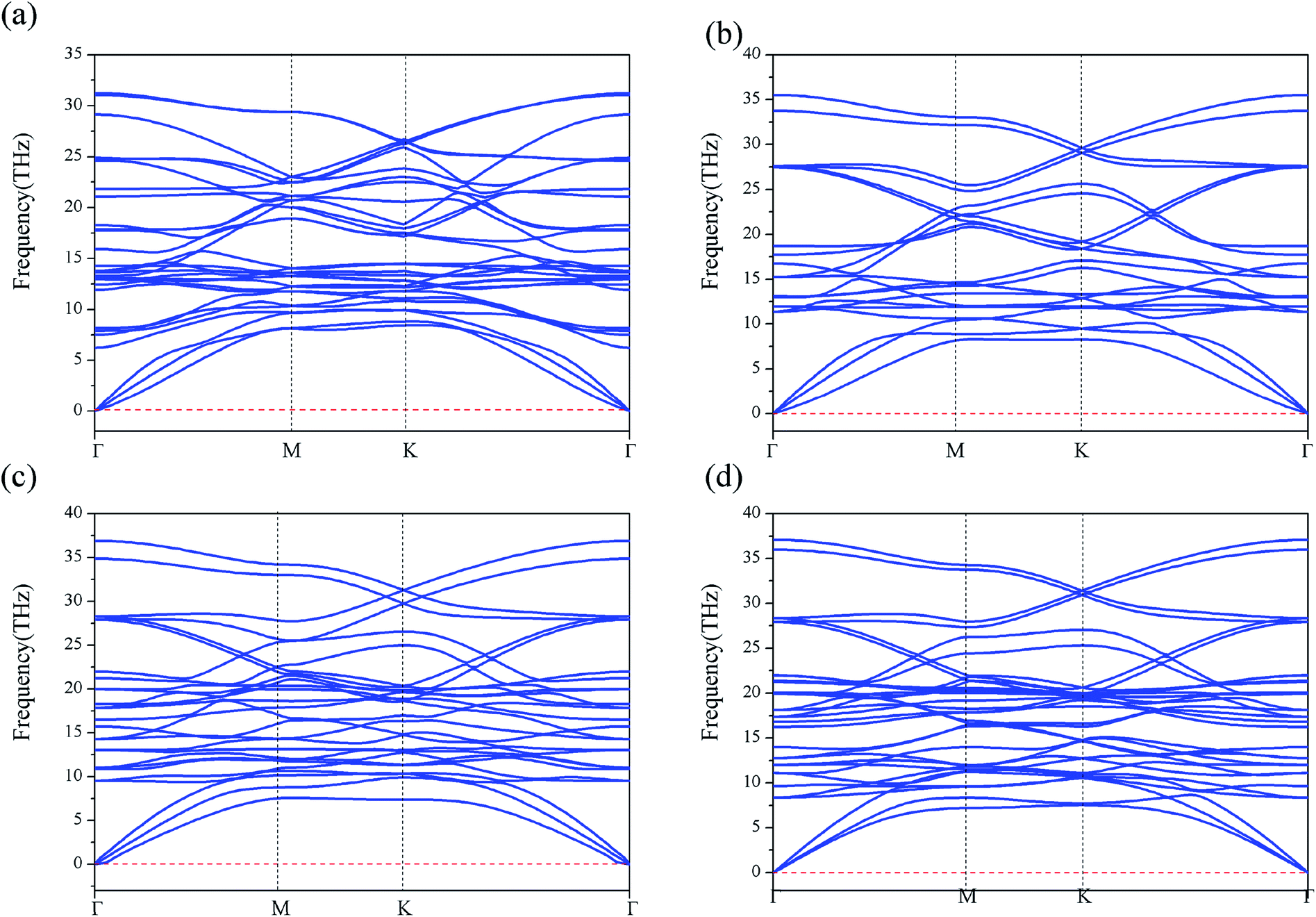Fig. 2 The phonon band dispersions for the iron borides FeB_x sandwich structures. (a–d) Represent the phonon dispersion of FeB₄, FeB₆, FeB₈ and FeB₁₀, respectively.

3.2 Electronic properties of iron borides FeB_x

In order to explore the electronic properties of iron borides FeB_x, we calculated the electronic band structure of these compounds by the PBE functional. We compared the band structures of PBE with/without SOC and found that SOC effect could be ignored since it had little impact to the band structure of iron borides FeB_x. As the PBE functionals are known to underestimate the bandgap of semiconductors, we applied the HSE06 as the exchange–correlation functional to obtain the accurate bandgaps of these compounds.

As shown in the Fig. 3a, the HSE06 calculated bandgap is 3.36 eV for FeB₆. According to the band structures shown in Fig. S6,† all these semiconductors own indirect bandgaps, 2.36, 3.51, 3.44 eV for FeB₄, FeB₈, FeB₁₀, respectively. With the D_6h symmetry of FeB₆ sandwich, the Fe 3d orbitals split into E_1g(d_xy, d_x²−y²), E_2g(d_xz, d_yz), A_1g(d_z²) in the triangular lattice, while the s, p orbitals of B in the kagome lattice are tend to form the in-plane sp² hybridize orbital and the out-of-plane p_z orbital. Using the WANNIER90 package^49,50 with these projection orbitals, we fit a tight-binding (TB) Hamiltonian with maximally localized Wannier functions to the bands calculated by the first-principles method (red dash line in Fig. 3a), indicating the dominant contributions of these orbitals to the electronic properties for FeB₆. The valence-band maximum (VBM) is along the K–Γ direction, and the conduction-band minimum (CBM) of FeB₆ occurs along the M–K direction. Insight in the PDOS of FeB₆ in Fig. 3b, the states near the Fermi level have contributions from the d_z² orbital of Fe and p_z orbital of B. While, the p_z orbital of B and (d_xz + d_yz) orbital of Fe dominate the states of VBM and CBM, which can be viewed from the charge distribution of VBM and CBM in Fig. 3c. The B crystal field increases the splitting of Fe 3d orbitals, and the PDOS indicates the strong hybridization between B p_z orbital and Fe d_z², d_xz + d_yz orbital. Note that the isolated bilayer B kagome lattice and Fe triangular lattice are both metallic, while the interactions between the Fe 3d orbital and B p_z orbital induce the semiconducting in these stable 2D sandwich structures.

Fig. 3 The electronic properties of FeB₆ sandwich. (a) Electronic band structure of FeB₆, the blue solid line represents the PBE band, the red dash line represents the Wannier interpolated band, the orange dash line represents the HSE06 band. (b) Total and partial densities of states (PDOS) of FeB₆ sandwich at HSE06 level. (c) Charge distribution of VBM and CBM for the FeB₆ sandwich at HSE06 level. The energy zero is set at the VBM for (a) and (b).

To understand the stabilities of these 2D materials, we studied the electron localization function (ELF) to gain a deep analysis of the unique bonding characteristics, as the ELF can present good description of electron localization in solids, which can help to highlight the bond distributions between B–B, B–Fe atoms. As shown in Fig. 4(a–d), the electrons are widely distributed around B atoms. The whole boron networks are covered by the delocalized electrons gas, with the charge transfer from Fe to boron. The isolated B monolayer on the surface of FeB₈ and FeB₁₀ lead to an intensive electron distributions as shown in the side view of Fig. 4(c and d). According to the Bader charge analysis method, it is found that each Fe atom transfers 0.192 e to the adjacent B atoms in the FeB₄ thin film. In the multilayers FeB_(6,8,10), the charge transfers are 0.236 e, 0.312 e, 0.332 e respectively, due to the electron deficiency of B kagome frame and moderate electronegativity of Fe.

Fig. 4 Isosurfaces of electron localization function (ELF) plotted with 60% of the peak amplitude value for the FeB_x sandwiches (HSE06). (a–d) Top and side view of the ELF maps for FeB_(4,6,8,10), the color from red to blue in the side view indicating accumulation and depletion of electrons.

3.3 Optical properties and vibrational mode

Here we have studied the absorption spectra of iron borides FeB_x sandwiches semiconductors with the HSE06 functional to explore the potential application in optoelectronic devices. First, the frequency-dependent dielectric function ε(ω) = ε₁(ω) + iε₂(ω) is calculated, and then the absorption coefficient as a function of photon energy is evaluated according to the following expression.^51,52

As shown in Fig. 5a, the large bandgap semiconductor corresponds to a blueshift absorption spectra, compared to 2D semiconductors black phosphorus⁵³ and MoS₂.⁵⁴ For potential application in real systems, the 2D semiconductors should be grown on a flexible substrate, where the strain effect would inevitably be considered due to the lattice constant mismatch. Here we simulated the strain effect for FeB₆ (the most stable semiconductor in the phase diagram). Negative and positive values of σ stand for compression and elongation, respectively. As the bandgap are tunable by the strain effect, here we calculated the HSE06 bandgap as a function of σ, shown in Fig. 5b inset with a reasonable strain ranging form −5% to 5%. The bandgap of FeB₆ sandwich would be effectively modulated with the biaxial strain, from 1.6 eV to 3.5 eV. As shown in Fig. 5b, the absorption spectra of FeB₆ without strain is located in the ultraviolet region. Under compression, the absorption spectra are blueshifted, while there are redshift with the tensile strain. The other three semiconductors presented a similar phenomenon shown in the Fig. S7.† The optical properties can be effectively modulated by changing of bandgap with the various biaxial strain, where the tensile strain will reduce the gap and result in the absorption of photo energy at the blue-purple light region, indicating a promising for efficient thin film ultrathin solar-cell applications.

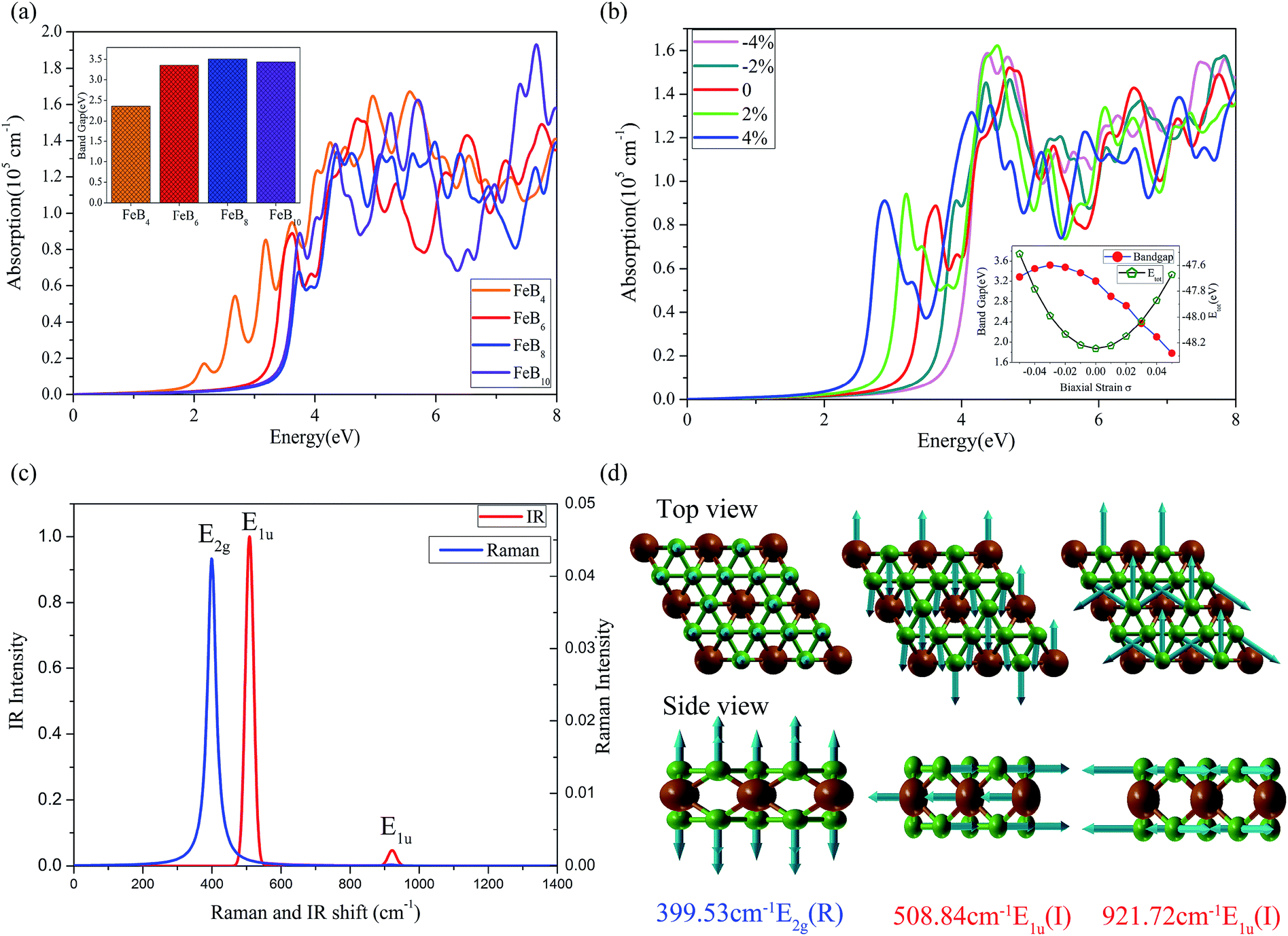Fig. 5 The optical properties (HSE06) and vibrational mode for the stable semiconductors. (a) The absorption spectra of 2D FeB_x (x = 4, 6, 8, 10) sandwiches. (b) Strain induced change of the absorption spectra of 2D FeB₆, inset represents the band gap and total energy of FeB₆ as a function of biaxial strain σ. (c) The simulated Raman and IR spectra for FeB₆. (d) The Raman and IR vibrational modes for the corresponding intensity peaks.

Based on Density-Functional Perturbation Theory (DFPT)⁵⁵ linear response calculations, we simulated the Raman and Infrared (IR) spectra of FeB₆ sandwich at the Γ point in the Brillouin zone center. There are 21 representations for FeB₆ [P6/mmm(191)], analyzed by the Phonopy code,^42,43 the irreducible representations of the Γ point and can be expressed as

Γ = 3A_u ⊕ 4E_1g(R) ⊕ 3E_2g(R) ⊕ A_1g(R) ⊕ B_1g(R) ⊕ 5E_1u(I) ⊕ 2E_2u(I) ⊕ A_2u(I) ⊕ B_2u(I)

The E_1g, E_2g, A_1g, and B_1g are Raman-active, E_1u, E_2u, A_2u, B_2u are Infrared-active, and A_u is neither Raman nor Infrared active. The calculated Raman and IR vibrational modes with corresponding wave numbers are presented in Fig. 5c. The vibrational modes for the intense peaks are plotted in Fig. 5d, which shows that the out-of-plane vibration of the B kagome lattice leads to the Raman E_2g active mode at 399.53 cm⁻¹ and in-plane vibration of B and Fe atoms corresponding to the IR active mode at 508.84 cm⁻¹. Finally, the multiple in-plane vibration of B atoms results in a small IR active peak at 921.72 cm⁻¹. Raman active mode is very useful to access the information of the anisotropic polarization-dependence properties for the 2D semiconductors. The analysis of Raman scattering intensity for FeB₆ is presented in Fig. S8.† The Raman and IR active mode may be useful to experimentally identify the 2D semiconductors in the future.

4. Conclusion

In summary, we have confirmed that the structures of the stable 2D iron borides FeB_x are multilayer structures through the USPEX search combined with the DFT calculation. By using HSE06 functional, we carried out the band structure calculation and found the stable FeB_(4,6,8,10) are 2D wide-band-gap semiconductors. In addition, we notice that, the bandgap and optical properties of FeB₆ sandwich can be effectively adjusted by applying a biaxial strain, through the tensile strain, the range of the absorption spectra extends from the UV region to the blue-purple light region. Finally, we also calculate the Raman and IR vibrational modes for FeB₆ sandwich, which may offer a few guidance for the experimental characterization.

Acknowledgements

This work was supported by National Natural Science Foundation of China (No. 11474100, 11674148), Guangdong Natural Science Funds for Distinguished Young Scholars (No. 2014A030306024), and the Basic Research Program of Science, Technology and Innovation Commission of Shenzhen Municipality (Grant No. JCYJ20160531190054083).

References

1. A. N. Alexandrova, A. I. Boldyrev, H. J. Zhai and L. S. Wang, Coord. Chem. Rev., 2006, 250, 2811–2866.
2. A. P. Sergeeva, I. A. Popov, Z. A. Piazza, W. L. Li, C. Romanescu, L. S. Wang and A. I. Boldyrev, Acc. Chem. Res., 2014, 47, 1349–1358.
3. L. S. Wang, Int. Rev. Phys. Chem., 2016, 35, 69–142.
4. W. Huang, A. P. Sergeeva, H.-J. Zhai, B. B. Averkiev, L.-S. Wang and A. I. Boldyrev, Nat. Chem., 2010, 2, 202–206.
5. A. P. Sergeeva, Z. A. Piazza, C. Romanescu, W. L. Li, A. I. Boldyrev and L. S. Wang, J. Am. Chem. Soc., 2012, 134, 18065–18073.
6. W. L. Li, Y. F. Zhao, H. S. Hu, J. Li and L. S. Wang, Angew. Chem., Int. Ed. Engl., 2014, 53, 5540–5545.
7. W. L. Li, Q. Chen, W. J. Tian, H. Bai, Y. F. Zhao, H. S. Hu, J. Li, H. J. Zhai, S. D. Li and L. S. Wang, J. Am. Chem. Soc., 2014, 136, 12257–12260.
8. Z. A. Piazza, H. S. Hu, W. L. Li, Y. F. Zhao, J. Li and L. S. Wang, Nat. Commun., 2014, 5, 3113.
9. W. L. Li, R. Pal, Z. A. Piazza, X. C. Zeng and L. S. Wang, J. Chem. Phys., 2015, 142, 204305.
10. J. Lv, Y. Wang, L. Zhu and Y. Ma, Nanoscale, 2014, 6, 11692–11696.
11. H. J. Zhai, Y. F. Zhao, W. L. Li, Q. Chen, H. Bai, H. S. Hu, Z. A. Piazza, W. J. Tian, H. G. Lu, Y. B. Wu, Y. W. Mu, G. F. Wei, Z. P. Liu, J. Li, S. D. Li and L. S. Wang, Nat. Chem., 2014, 6, 727–731.
12. Q. Chen, W.-L. Li, Y.-F. Zhao, S.-Y. Zhang, H.-S. Hu, H. Bai, H.-R. Li, W.-J. Tian, H.-G. Lu, H.-J. Zhai, S.-D. Li, J. Li and L.-S. Wang, ACS Nano, 2015, 9, 754–760.
13. C. Romanescu, T. R. Galeev, A. P. Sergeeva, W.-L. Li, L.-S. Wang and A. I. Boldyrev, J. Organomet. Chem., 2012, 721–722, 148–154.
14. C. Romanescu, T. R. Galeev, W.-L. Li, A. I. Boldyrev and L.-S. Wang, Angew. Chem., Int. Ed., 2011, 50, 9334–9337.
15. W.-L. Li, C. Romanescu, T. R. Galeev, Z. A. Piazza, A. I. Boldyrev and L.-S. Wang, J. Am. Chem. Soc., 2012, 134, 165–168.
16. T. R. Galeev, C. Romanescu, W.-L. Li, L.-S. Wang and A. I. Boldyrev, Angew. Chem., Int. Ed., 2012, 51, 2101–2105.
17. I. A. Popov, T. Jian, G. V. Lopez, A. I. Boldyrev and L. S. Wang, Nat. Commun., 2015, 6, 8654.
18. T. Jian, W.-L. Li, I. A. Popov, G. V. Lopez, X. Chen, A. I. Boldyrev, J. Li and L.-S. Wang, J. Chem. Phys., 2016, 144, 154310.
19. W. L. Li, T. Jian, X. Chen, T. T. Chen, G. V. Lopez, J. Li and L. S. Wang, Angew. Chem., Int. Ed., 2016, 55, 7358–7363.
20. T. Jian, W.-L. Li, X. Chen, T.-T. Chen, G. V. Lopez, J. Li and L.-S. Wang, Chem. Sci., 2016, 7, 7020–7027.
21. H. Tang and S. Ismail-Beigi, Phys. Rev. Lett., 2007, 99, 115501.
22. X. Yang, Y. Ding and J. Ni, Phys. Rev. B: Condens. Matter Mater. Phys., 2008, 77, 041402.
23. S. G. Xu, Y. J. Zhao, J. H. Liao, X. B. Yang and H. Xu, Nano Res., 2016, 9, 2616–2622.
24. Z. Zhang, Y. Yang, G. Gao and B. I. Yakobson, Angew. Chem., Int. Ed. Engl., 2015, 53, 13022–13026.
25. H. Shu, F. Li, P. Liang and X. Chen, Nanoscale, 2016, 8, 16284–16291.
26. A. J. Mannix, X.-F. Zhou, B. Kiraly, J. D. Wood, D. Alducin, B. D. Myers, X. Liu, B. L. Fisher, U. Santiago, J. R. Guest, M. J. Yacaman, A. Ponce, A. R. Oganov, M. C. Hersam and N. P. Guisinger, Science, 2015, 350, 1513–1516.
27. B. J. Feng, J. Zhang, Q. Zhong, W. B. Li, S. Li, H. Li, P. Cheng, S. Meng, L. Chen and K. H. Wu, Nat. Chem., 2016, 8, 564–569.
28. L. Z. Zhang, Z. F. Wang, S. X. Du, H. J. Gao and F. Liu, Phys. Rev. B: Condens. Matter Mater. Phys., 2014, 90, 161402.
29. S.-Y. Xie, X.-B. Li, W. Q. Tian, N.-K. Chen, X.-L. Zhang, Y. Wang, S. Zhang and H.-B. Sun, Phys. Rev. B: Condens. Matter Mater. Phys., 2014, 90, 035447.
30. X. Zhang, J. Hu, Y. Cheng, H. Y. Yang, Y. Yao and S. A. Yang, Nanoscale, 2016, 8, 15340–15347.
31. C. Wu, H. Wang, J. J. Zhang, G. Y. Gou, B. C. Pan and J. Li, ACS Appl. Mater. Interfaces, 2016, 8, 2526–2532.
32. H. J. Zhang, Y. F. Li, J. H. Hou, K. X. Tu and Z. F. Chen, J. Am. Chem. Soc., 2016, 138, 5644–5651.
33. H. Zhang, Y. Li, J. Hou, A. Du and Z. Chen, Nano Lett., 2016, 16, 6124–6129.
34. A. R. Oganov and C. W. Glass, J. Chem. Phys., 2006, 124, 244704.
35. C. W. Glass, A. R. Oganov and N. Hansen, Comput. Phys. Commun., 2006, 175, 713–720.
36. Q. Zhu, L. Li, A. R. Oganov and P. B. Allen, Phys. Rev. B: Condens. Matter Mater. Phys., 2013, 87, 195317.
37. G. Kresse and J. Hafner, Phys. Rev. B: Condens. Matter Mater. Phys., 1993, 47, 558–561.
38. G. Kresse and J. Furthmüller, Phys. Rev. B: Condens. Matter Mater. Phys., 1996, 54, 11169–11186.
39. G. Kresse and D. Joubert, Phys. Rev. B: Condens. Matter Mater. Phys., 1999, 59, 1758–1775.
40. J. P. Perdew, K. Burke and M. Ernzerhof, Phys. Rev. Lett., 1996, 77, 3865–3868.
41. J. Heyd, G. E. Scuseria and M. Ernzerhof, J. Chem. Phys., 2003, 118, 8207–8215.
42. K. Parlinski, Z. Q. Li and Y. Kawazoe, Phys. Rev. Lett., 1997, 78, 4063–4066.
43. A. Togo, F. Oba and I. Tanaka, Phys. Rev. B: Condens. Matter Mater. Phys., 2008, 78, 134106.
44. S. Nosé, J. Chem. Phys., 1984, 81, 511–519.
45. T. P. Martin, Phys. Rep., 1983, 95, 167.
46. J. Li, Y. Wei, X. Fan, H. Wang, Y. Song, G. Chen, Y. Liang, V. Wang and Y. Kawazoe, J. Mater. Chem. C, 2016, 4, 9613–9621.
47. S.-Y. Xie, X.-B. Li, W. Q. Tian, N.-K. Chen, Y. Wang, S. Zhang and H.-B. Sun, Phys. Chem. Chem. Phys., 2015, 17, 1093–1098.
48. X.-B. Li, S.-Y. Xie, H. Zheng, W. Q. Tian and H.-B. Sun, Nanoscale, 2015, 7, 18863–18871.
49. N. Marzari, A. A. Mostofi, J. R. Yates, I. Souza and D. Vanderbilt, Rev. Mod. Phys., 2012, 84, 1419–1475.
50. A. A. Mostofi, J. R. Yates, Y.-S. Lee, I. Souza, D. Vanderbilt and N. Marzari, Comput. Phys. Commun., 2008, 178, 685–699.
51. J.-H. Lin, H. Zhang, X.-L. Cheng and Y. Miyamoto, Phys. Rev. B, 2016, 94, 195404.
52. S. Saha, T. P. Sinha and A. Mookerjee, Phys. Rev. B: Condens. Matter Mater. Phys., 2000, 62, 8828–8834.
53. D. Çakır, C. Sevik and F. M. Peeters, Phys. Rev. B: Condens. Matter Mater. Phys., 2015, 92, 165406.
54. H. Shi, H. Pan, Y.-W. Zhang and B. I. Yakobson, Phys. Rev. B: Condens. Matter Mater. Phys., 2013, 87, 155304.
55. S. Baroni, S. de Gironcoli, A. Dal Corso and P. Giannozzi, Rev. Mod. Phys., 2001, 73, 515–562.

---

Footnote

† Electronic supplementary information (ESI) available. See DOI: 10.1039/c7ra03153j

---