DOI:
10.1039/C7RA00417F
(Paper)
RSC Adv., 2017,
7, 12407-12418
Franck–Condon simulation for unraveling vibronic origin in solvent enhanced absorption and fluorescence spectra of rubrene†
Received
11th January 2017
, Accepted 14th February 2017
First published on 21st February 2017
Abstract
Quantum chemistry calculations at the level of (TD)-DFT plus PCM solvent models are employed for analyzing potential energy surfaces and as a result two local minima with D2, two local minima with C2H, and one second-order transition state with D2H group symmetry are found in both ground S0 and excited-state S1 potential energy surfaces. Simulated vibronic coupling distributions indicate that only second-order transition states with D2H group symmetry are responsible for observed absorption and fluorescence spectra of rubrene and vibrational normal-motions related with atoms on the aromatic backbone are active for vibronic spectra. The Stokes shift 1120 cm−1 (820 cm−1) and vibronic-band peak positions in both absorption and fluorescence spectra in non-polar benzene (polar cyclohexane) solvent are well reproduced within the conventional Franck–Condon simulation. By adding damped oscillator correction to Franck–Condon simulation, solvent enhanced vibronic-band intensities and shapes are well reproduced. Four (three) normal modes with vibration frequency around 1550 cm−1 (1350 cm−1) related to ring wagging plus CC stretching and CH bend motions on the backbone are actually interpreted for solvent enhanced absorption (fluorescence) spectra of rubrene in benzene and cyclohexane solutions.
1. Introduction
Franck–Condon (FC) factors play a very important role for theoretical modeling and interpreting experimental observations for irradiative processes like electronic spectra of VUV absorption and fluorescence as well as the nonradiative processes like electron and energy transfer.1–10 For large polyatomic molecules, multidimensional Franck–Condon overlapping integrals are conventionally decomposed into a product of one-dimensional Franck–Condon overlap integrals in terms of normal mode coordinates under harmonic oscillator approximation. Harmonic oscillator approximation provides the leading-term contribution to FC factors, and further higher order corrections of distorted oscillator approximation and mode-mixing including Duschinsky effect and anharmonic oscillators have been introduced to improve FC factors and its various applications.11–17 Most of the electronic molecular spectra and vibrational relaxation processes are experimentally carried out in solution phases. Therefore, theoretical modeling can deal with solutes and solvent molecules separately and FC factors including electronic and nuclear parts are treated separately as well. The electronic parts involve calculating electronic transition dipole momentum and nonadiabatic coupling matrix under solvent environment: the most popular theoretical approach is represented by continuum solvation models, especially the polarizable continuum model (PCM) combined with time-dependent density functional theory (TDDFT). The (TD)-DFT plus PCM approach provides an accurate simulation of static electronic potential energy surfaces of both ground and excited states for molecules in solution. The nuclear parts represent dynamic motion and its FC factors have been investigated based on various corrections to the leading-term FC factors.18–36 By introducing damped harmonic oscillator approximation, Zhu and co-authors36 formulated the empirical correction to each normal mode differently in solvent environment by converting the mass-weighted unperturbed gas-phase Hessian matrix to solution-phase perturbed Hessian matrix. This method is based on idea that each normal-mode motion can be affected differently in solution, however each local-mode motion can be affected in quite similar way for highly symmetric molecules like polycyclic aromatic hydrocarbon molecules in which CH-stretch local modes, for example, are considered as in the same solvent environment. This method was previously demonstrated for interpreting solvent enhanced absorption and fluorescence spectra of perylene in benzene solution by applying a single empirical parameter to CH-stretch local modes.36
One of the purposes in the present study is to continue damped harmonic oscillator FC simulation for much large size of polycyclic aromatic hydrocarbon like rubrene. The other is to interpret experimentally observed vibronic spectra in terms of potential energy surfaces of ground and excited states, transition patterns, molecular structure, solvent dependence and so on. For instance, it is traditionally considered that vibronic spectra simulated by FC factors are based on local minima between ground- and excited-state potential energy surfaces, and this is usually true for rigid molecules. However, for flexible molecules, potential energy surfaces are very complicated with many local minima closed to one another, in this case, (high-order) transition states that connect (more than) two local minima can play crucial role in FC simulation in order to interpret observed vibronic spectra.
Rubrene molecules have been attracted more attention in the field of organic semiconductor because of its high mobility at room temperature and optical properties, and rubrene can be used as a laser dye and a fluorescent dopant in organic light emitting devices, field effect transistors and solar cell.37–46 In the present study we focus on the optical properties of monomer of rubrene in non-polar benzene and polar cyclohexane solvents. Rubrene molecule is constructed with four six-member rings as the aromatic backbone connected by four phenyl rings perpendicular to the backbone. The backbone is the fluorescent center that can have planar or twisted geometry, and its optical spectra, however, are not well understood in terms of structure of the backbone geometry as well as phenyl groups. Moreover, it is well-know that rubrene has the large Stokes shift, but what is dependence in terms of solvent environment. We investigate how solvent enhanced absorption and fluorescence spectra vary with respect to solvents by damped FC simulation and identify physical origin of vibronic spectra in terms of ground- and excited-sate potential energy surfaces.
The rest of this paper is organized as follows: Section 2 briefly introduces damped harmonic oscillator FC factors and discuss (TD)-DFT+ PCM method for calculating potential energy surfaces of ground and excited states for rubrene molecule. Section 3 discusses how to reproduce experimentally observed absorption and fluorescence spectra in benzene and cyclohexane solution, and to interpret vibronic spectra in terms of molecular structure, molecular orbitals, vibrational normal modes and solvent environment. Section 4 presents concluding remarks.
2. Damped Franck–Condon factors
Within displaced harmonic oscillator approximation, absorption and fluorescence coefficients can be analytically derived as follows:1,42| |
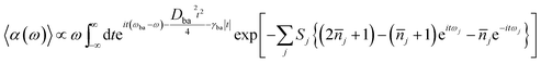 | (1) |
and
| |
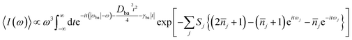 | (2) |
where
ωba represents electronically adiabatic excitation energy between electronic states b and a.
is the average phonon distribution,
γba is the homogeneous broadening parameter and
Dba is inhomogeneous broadening parameter that reflects static interaction between electronic states of molecule and solvent, and
ωj is the
j-th normal mode vibrational frequency. The dimensionless Huang–Rhys factor
Sj corresponding to the
j-th normal mode is defined as
| |
 | (3) |
where displacement
dj is given by
| |
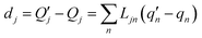 | (4) |
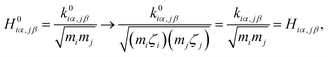
The  and qn in eqn (4) are the mass-weighted Cartesian coordinates at equilibrium geometries (or transition states) of the electronic excited and ground states, respectively. Transformation matrix L in eqn (4) can be computed with frequency analysis using G09 programs, for instance. By applying damped diatomic harmonic oscillator to local-mode force constant of gas-phase Hessian matrix Hij, we formulate damped FC factors as transferring the mass-weighted gas-phase unperturbed Hessian matrix to solvent perturbed Hessian matrix,36
| |
 | (5) |
where
mi and
mj are atomic mass, and
α and
β are Cartesian component (
x,
y,
z) of the position of nucleus
i and
j. Unperturbed local force constant

is converted to perturbed force constant
. The dimensionless scaling parameter
ζj in
eqn (5) is treated as an empirical parameter that can be considered as a local dynamic interaction of atom
j of solute molecule with solvent molecules. By diagonalizing perturbed Hessian matrix in
eqn (5), we obtain normal mode frequencies and transformation matrix (that transfers the mass-weighted Cartesian coordinates to normal mode coordinates) corresponding to solute molecule under the solvent environment. It should be emphasized that solvent effect by damped oscillator can directly modify the leading-term of FC factors, so that it is usually larger than the other effects such as distorted oscillator, Duschinsky effect and anharmonic effect which are in higher-order perturbation terms.
We have employed the (time-dependent) density functional theory with functional (TD)-B3LYP47 (i.e., B3LYP20), (TD)B3LYP35, (TD)-B3LYP50 (i.e., BHandHLYP),48 and HF–CIS (i.e., B3LYP100) plus PCM condition in benzene and cyclohexane solvents for calculating potential energy surfaces of ground and the first excited states. The numbers following after B3LYP stand for different hybrid exchange–correlation functionals containing 20% (B3LYP), 35%, 50%, and 100% of exact Hartree–Fock exchange in the density functional theory. The basis set is chosen as 6-31G throughout all calculations and all calculations are carried out using GAUSSIAN 09 program package.49 Calculations from four functionals given above lead to the same conclusion in which there are two local minima with D2, two local minima with C2H, and one second-order transition state with D2H group symmetry in both ground- and excited-state potential energy surfaces. This conclusion does hold for PCM condition in both non-polar benzene and polar cyclohexane solvents although electronic structures can vary slightly. From preliminary vibronic spectral calculation, we found that (TD)-B3LYP50 presents the best agreement with experimental results among four functionals, and this is the same as results obtained in ref. 42. However, there is important difference in comparison with ref. 42 in which there are only two local minima, one is in D2 and the other is in D2H symmetry (note for this point, we show it is second-order transition state). The Huang–Rhys factors calculated from our D2H structure are similar to those from their D2H symmetry, but the Huang–Rhys factors calculated from our D2 structure are very different to those from their D2 symmetry. Actually, the second-order transition point at D2H connects two local minima at D2 as well as two local minima at C2H, and we will discuss this in detail later. In the following discussions, we only report calculations from (TD)-BHandHLYP (B3LYP50) as it performs best for vibronic spectral simulations.
3. Results and analysis
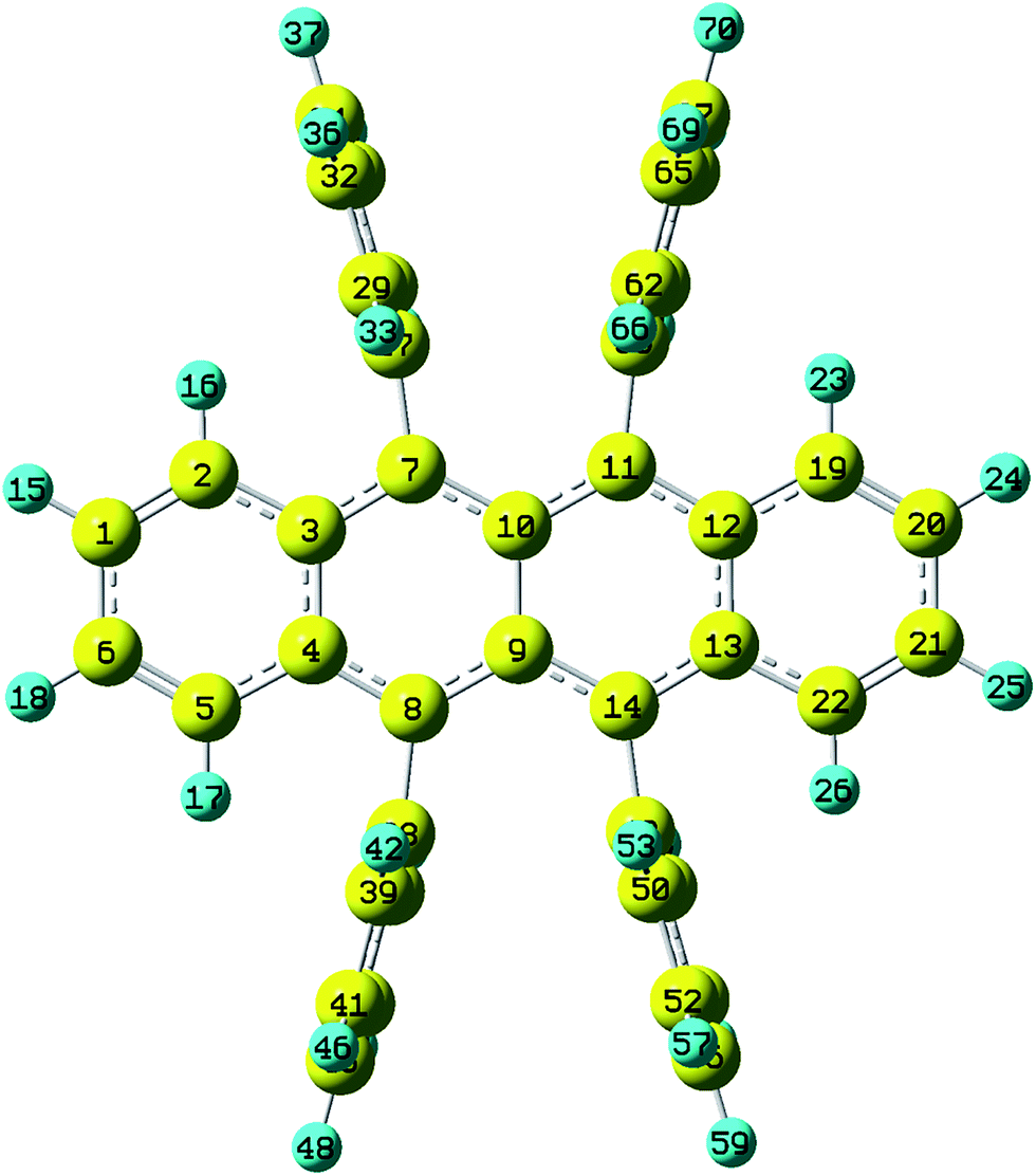
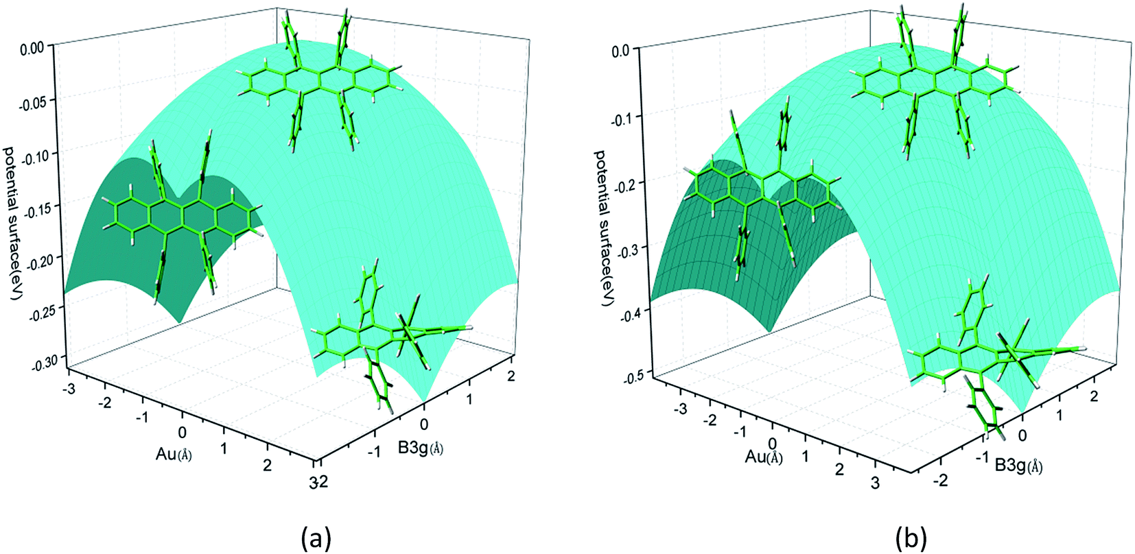
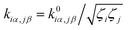
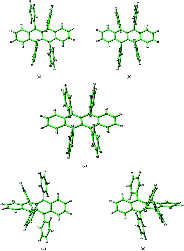
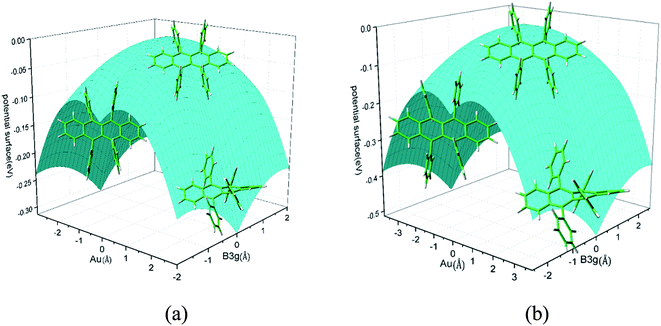
Rubrene molecule plays as a prototype of large-size polycyclic aromatic hydrocarbon molecules for a better understanding of molecular structure, spectra, dynamics, solvent effect, and so on. It's highly symmetrical electronic structures (see atomic numbering in Fig. 1) in which all hydrogen atoms are approximately subjected to the same environment interacting with solvent molecules and this greatly simplifies empirical search of the scaling parameters in damped FC simulation. Geometry of rubrene molecule is composed with four linearly connected six-member rings as aromatic backbone connected by four phenyl rings perpendicular to the backbone. The present (TD)-DFT calculations reveal that there are two local minima at C2H group symmetry where C2H(1) minimum is mirror image of C2H(2) minimum as shown in Fig. 2(a) and (b), there is one second-order transition state at D2H group symmetry as shown in Fig. 2(c), and there are two local minima at D2 group symmetry where D2(1) minimum is mirror image of D2(2) minimum as shown in Fig. 2(d) and (e). These kind of electronic conformers displayed in Fig. 2 show similar structures for ground and excited states in both benzene and cyclohexane solvents. At D2H transition state, there are actually two normal modes with imaginary frequencies −58.62 cm−1 and −54.49 cm−1 (−58.06 cm−1 and −53.21 cm−1) in Au and B3G symmetries, respectively for the ground (excited) state in benzene solvent. Along Au and B3G normal-mode coordinates, we draw two-dimensional potential energy surface diagrams in which second-order D2H transition state connects two D2 minima via Au and two C2H minima via B3G as shown in Fig. 3(a) for ground state and Fig. 3(b) for excited state in benzene solvent environment. Similar potential energy surface diagrams in cyclohexane solvent environment are also shown in Fig. 4(a) and (b), where two imaginary frequencies are −56.54 cm−1 and −52.85 cm−1 (−55.70 cm−1 and −51.29 cm−1) with Au and B3G mode symmetries, respectively for the ground (excited) state. Difference between ground and excited state potential energy surfaces is not large, and this confirms that the present displaced harmonic FC simulation should be good approximation to reproduce experimental vibronic spectra. The adiabatic potential energy gap between D2H-transition state and D2-local minima (C2H-local minima) is 0.31 eV (0.12 eV) as shown in Fig. 3(a) and 4(a) for S0 state and is 0.51 eV (0.20 eV) as shown in Fig. 3(b) and 4(b) for S1 state, respectively in both benzene and cyclohexane solvents. Potential energy surfaces around D2H-transition state in terms of two imaginary normal-mode coordinates show little dependence on solvent.
 |
| | Fig. 1 Atomic numbering (optimized geometries under D2H group symmetry by BHandHLYP/6-31G plus PCM model. The yellow and blue indicate carbon and hydrogen atoms respectively). | |
 |
| | Fig. 2 Optimized geometries by BHandHLYP/6-31G plus PCM model in benzene solvent for ground-state S0. Local minima (a) C2H(1) and (b) C2H(2), (c) second-order transition state D2H, and local minima (d) D2(1) and (e) D2(2). | |
 |
| | Fig. 3 Potential energy surface along two imaginary normal-mode coordinates (Au and B3G symmetries) starting from D2H transition state point which connects two C2H minima via B3G-mode direction, and two D2 minima via Au-mode direction. (a) Ground state and (b) excited state in benzene solvent. | |
 |
| | Fig. 4 Potential energy surface along two imaginary normal-mode coordinates (Au and B3G symmetries) starting from D2H transition state point which connects two C2H minima via B3G-mode direction, and two D2 minima via Au-mode direction. (a) Ground state and (b) excited state in cyclohexane solvent. | |
3.1. Electronic structures, potential energy surfaces and the Huang–Rhys factors
The present (TD)-DFT+ PCM calculations reveal that the backbone formed by the four six-member rings is planar structure at local minima C2H(1), C2H(2) and the second-order transition state D2H, but the backbone is twisted at local minima D2(1) and D2(2) for both S0 and S1 states. Since there are existing D2, C2H and D2H group symmetries at five optimized geometries for both S0 and S1 states, the internal coordinates of selected bond lengths, bond angles and dihedral angles which well represent geometries of electronic structures contributing to vibronic spectra are given in Tables 1 and 2. Tables 1 and 2 actually show difference of bond lengths, bond angles and dihedral angles between S0 and S1 states with the same group symmetry in benzene and cyclohexane solvents, respectively, and the corresponding absolute values of those internal coordinates are shown in Tables S1 and S2† (Full Cartesian coordinates for optimized geometries shown in Table S3) (ESI†). As is well-known, the magnitude of Huang–Rhys factor defined in eqn (3) depends on the displacement of the normal mode between local minimum on ground state and corresponding local minimum on excited state, while the displacement of normal mode is converted from differences of internal coordinates between local minima of the ground and excited states. Bond-length differences vary with respect change of group symmetry from D2H to C2H and from D2H to D2 within small magnitude (the largest value is about 0.05 Å for C9C10 bond in benzene solvent) as shown in Tables 1 and 2, and this can lead the change of Huang–Rhys factor about 0.4. However, bond-angle differences can vary within as large as 6°, and this can lead to the change of Huang–Rhys factor about 4. The largest change happens for dihedral angles as shown in Tables 1 and 2 and it can go as large as ten degree, but these changes affect change of Huang–Rhys factor in complicated way and it is hard to predict the magnitude change before carrying out real calculations. This fact was actually confirmed in which the Huang–Rhys factors of the some vibrational modes can go as large as from 5 to 50 due to big change in dihedral angles for the two isomeric compounds.50 Dihedral angle differences between S0 and S1 states at D2H group symmetry are all equal to zero as shown in the middle column of Tables 1 and 2, and thus this indicates that observed vibronic spectra should be mostly affected by the planar backbone structure. We will confirm this issue later.
Table 1 Differences of bond lengths (in Å), bond angles and dihedral angles (in degree) between ground and excited states and numbers of S1 minus S0 are listed for optimized representative geometries within D2, D2H, and C2H group symmetries and all are computed by (TD)-BHandHLYP/6-31G plus PCM model in benzene solvent (the atom numbering is showed in Fig. 1)
| Parameters |
Conformations |
| D2(1) |
D2(2) |
D2H |
C2H(1) |
C2H(2) |
| B(1,2) |
0.0285 |
0.0285 |
0.0304 |
0.0288 |
0.0288 |
| B(1,6) |
−0.0315 |
0.0315 |
−0.0319 |
−0.0307 |
−0.0307 |
| B(1,15) |
−0.0004 |
0.0004 |
−0.0002 |
0.0001 |
0.0001 |
| B(2,3) |
−0.0304 |
0.0304 |
−0.0309 |
−0.2976 |
−0.2976 |
| B(2,16) |
0.0000 |
0.0000 |
0.0001 |
0.0001 |
0.0001 |
| B(3,4) |
−0.0072 |
0.0072 |
−0.0086 |
−0.0069 |
−0.0069 |
| B(3.7) |
0.0387 |
−0.0387 |
0.0346 |
0.0367 |
0.0367 |
| B(7,10) |
−0.0173 |
0.0173 |
−0.0098 |
−0.0095 |
−0.0095 |
| B(7,27) |
−0.0084 |
0.0084 |
−0.0037 |
−0.0076 |
−0.0076 |
| B(8,38) |
−0.0084 |
0.0084 |
−0.0043 |
−0.0076 |
−0.0076 |
| B(9,10) |
0.0638 |
−0.0638 |
0.0134 |
0.0009 |
0.0009 |
| B(39,42) |
−0.0002 |
0.0002 |
−0.0001 |
−0.0003 |
−0.0003 |
| A(1,2,3) |
0.1300 |
−0.1300 |
−0.0100 |
−0.0200 |
−0.0200 |
| A(2,3,4) |
0.4000 |
−0.4000 |
0.4300 |
0.4000 |
0.4000 |
| A(2,1,6) |
−0.4200 |
0.4200 |
−0.3600 |
−0.3900 |
−0.3900 |
| A(3,7,10) |
0.2500 |
−0.2500 |
0.8600 |
0.3000 |
0.3000 |
| A(4,3,7) |
−0.5600 |
0.5600 |
−0.7000 |
−0.9400 |
−0.9400 |
| A(7,10,9) |
−0.4000 |
0.4000 |
−0.2200 |
−0.0500 |
−0.0500 |
| D(3,7,27,29) |
8.1500 |
−8.1500 |
0.0000 |
9.4600 |
−7.9000 |
| D(4,8,38,39) |
6.1400 |
−6.1400 |
0.0000 |
−9.4600 |
7.9000 |
| D(2,3,4,8) |
−1.3900 |
1.3900 |
0.0000 |
−0.0200 |
0.0200 |
| D(3,7,10,11) |
−3.9100 |
3.9100 |
0.0000 |
−4.2600 |
4.2600 |
| D(1,2,3,4) |
1.0300 |
−1.0300 |
0.0000 |
−0.4600 |
0.4600 |
| D(7,10,9,8) |
4.7800 |
−4.7800 |
0.0000 |
0.0000 |
0.0000 |
Table 2 Differences of bond lengths (in Å), bond angles and dihedral angles (in degree) between ground and excited states and numbers of S1 minus S0 are listed for optimized representative geometries within D2, D2H and C2H group symmetries and all are computed by (TD)-BHandHLYP/6-31G plus PCM model in cyclohexane solvent (the atom numbering is showed in Fig. 1)
| Parameters |
Conformations |
| D2(1) |
D2(2) |
D2H |
C2H(1) |
C2H(2) |
| B(1,2) |
0.0286 |
0.0286 |
0.0404 |
0.0289 |
0.0289 |
| B(1,6) |
−0.0314 |
−0.0314 |
−0.0319 |
−0.0306 |
−0.0306 |
| B(1,15) |
−0.0003 |
−0.0003 |
−0.0002 |
−0.0002 |
−0.0002 |
| B(2,3) |
−0.0305 |
−0.0305 |
−0.0273 |
−0.0306 |
−0.0306 |
| B(2,16) |
0.0000 |
0.0000 |
0.0002 |
0.0002 |
0.0002 |
| B(3,4) |
−0.0071 |
−0.0071 |
−0.0086 |
−0.0068 |
−0.0068 |
| B(3.7) |
0.0387 |
0.0387 |
0.0346 |
0.0365 |
0.0365 |
| B(7,10) |
−0.0144 |
−0.0144 |
−0.0097 |
−0.0095 |
−0.0095 |
| B(7,27) |
−0.0084 |
−0.0084 |
−0.0038 |
−0.0075 |
−0.0075 |
| B(8,38) |
−0.0084 |
−0.0084 |
−0.0038 |
−0.0075 |
−0.0075 |
| B(9,10) |
0.0168 |
0.0168 |
0.0134 |
0.0010 |
0.0010 |
| B(39,42) |
−0.0002 |
−0.0002 |
0.0000 |
−0.0003 |
−0.0003 |
| A(1,2,3) |
0.1300 |
0.1300 |
−0.0100 |
−0.0200 |
−0.0200 |
| A(2,3,4) |
0.3900 |
0.3900 |
0.4300 |
0.4000 |
0.4000 |
| A(2,1,6) |
−0.9700 |
−0.9700 |
−0.4200 |
−0.3900 |
−0.3900 |
| A(3,7,10) |
0.2600 |
0.2600 |
0.8600 |
0.3200 |
0.3200 |
| A(4,3,7) |
−0.5700 |
−0.5700 |
−0.7000 |
−0.9300 |
−0.9300 |
| A(7,10,9) |
−0.4100 |
−0.4100 |
−0.1800 |
0.0500 |
0.0500 |
| D(3,7,27,29) |
8.1600 |
−8.1600 |
0.0000 |
9.2900 |
−7.7100 |
| D(4,8,38,39) |
6.1500 |
−6.1500 |
0.0000 |
−9.2900 |
7.7100 |
| D(2,3,4,8) |
−1.3600 |
1.3600 |
0.0000 |
−0.0200 |
0.0200 |
| D(3,7,10,11) |
−3.9000 |
3.9000 |
0.0000 |
−4.2200 |
4.2200 |
| D(1,2,3,4) |
0.9900 |
−0.9900 |
0.0000 |
−0.4600 |
0.4600 |
| D(7,10,9,8) |
4.7800 |
−4.7800 |
0.0000 |
0.0000 |
0.0000 |
Experimentally observed absorption and fluorescence spectra in benzene and cyclohexane solvents are mostly from the lowest singlet excited state S1 of rubrene molecule with transition type of molecular orbital π → π*. The present calculations show that the first excited state S1 has π → π* feature, and natural orbital analysis confirm that the S1 state results mainly in the excitation of the HOMO → LUMO (one electron excited) as shown in Fig. S1 (ESI†) corresponding to S0 (X 1Ag) → S1 (A 1B3u) electronic excitation between S0-D2H and S1-D2H transition states. Fig. S1 (ESI†) show that electron density is located on the backbone in both HOMO and LUMO, so that four phenyl groups perpendicular to the backbone are not active for vibronic spectra. Therefore, this indicates that absorption and fluorescence spectra are mostly influenced by electronic transition associate with the backbone of rubrene, and solvent enhanced vibronic spectra should be also focused on carbon and hydrogen atoms in the backbone. Actually, the present (TD)-DFT calculations shows that adiabatic (vertical) excitation energies are 2.506 eV and 2.514 eV (2.753 eV and 2.760 eV) in benzene and cyclohexane solvents, respectively. Due to the backbone of rubrene is rigid frame, polar and non-polar solvents do not affect electronic excitation and even oscillator strengths are about the same as 0.33 for S0 (X 1Ag) → S1 (A 1B3u) excitation. The present (TD)-DFT calculations show good agreement with experimental data and the other theoretical calculations as shown in Table 3.
Table 3 Observed and calculated vertical and adiabatic excitation energies (Evert (eV) and Ead (eV)) with corresponding oscillator strengths (f) for 1B3u transition and discrepancies (Δ) between adiabatic excitation energies from theory and experiment
| Solvent |
Vertical |
Adiabatic |
| Evert |
f |
Ead (eV) |
Δ (eV) |
| Experiment values from ref. 42. Calculated values from ref. 42. |
| Benzene |
2.753 |
0.338 |
2.506 |
|
| Cyclohexane |
2.487a |
0.13a |
2.302a |
|
| 2.760 |
0.328 |
2.514 |
0.21 |
| 2.795b |
0.32b |
2.599b |
0.29 |
Franck–Condon factors can be qualitatively estimated from Huang–Rhys factors S (that are also called as vibronic coupling); when S is smaller than 1, peak position of vibronic spectra is close to adiabatic excitation energy ωba (or 0–0 vibronic transition energy), and when S is larger than 1, the peak position is far from ωba, and the larger S is, the farther from ωba. Therefore, Huang–Rhys factors can present an immediate comparison with experimentally observed spectra to determine which electronic structure is an actually contributed observed spectrum. Let us calculate Huang–Rhys factors based on S0-D2(1) and S1-D2(1) local minima (it is the same based on S0-D2(2) and S1-D2(2)), then we found there are S = 15 and S = 13 that correspond to vibrational frequencies 1565 cm−1 and 3331 cm−1, respectively in both benzene and cyclohexane solvents and its vibrational normal-mode motions are related to large change of dihedral angles in phenyl rings as shown in Fig. S2 (ESI†). Such large Huang–Rhys factors present vibronic spectra totally wrong in comparison with experimental results and actually peak positions of vibronic spectra in experiment tell that all S values should be smaller than unity. The same is also true if we analyze calculated Huang–Rhys factors based on S0-C2H(1) and S1-C2H(1) local minima, because there are S = 23 and S = 13 that correspond to vibrational frequencies 1563 cm−1 and 3330 cm−1 respectively, and its normal-mode motions are as shown in Fig. S3(ESI†). We performed fluorescence spectral calculations based on both D2 and C2H symmetries and that Huang–Rhys factors computed from S1-D2 and S1-C2H local minima also show very large S values as discussed as above for absorption spectrum. Thus, we conclude that observed vibronic spectra cannot be interpreted by molecular structures related to D2 and C2H group symmetries.
Only when we calculate Huang–Rhys factors based on the second-order transition states of S0-D2H and S1-D2H, we have all S values are smaller than unity as shown in Tables 4 and 6, and thus it is only D2H group symmetry that can interpret experimentally observed vibronic spectra. In the following sub-sections, we will discuss Franck–Condon simulation based on only the second-order transition states of D2H group symmetry. By performing frequency calculation at geometry of second-order transition state S0 (S1) in benzene solvent environment, we found 23 (21) total symmetry Ag vibrational modes with non-zero S values, while in cyclohexane solvent environment, we found 20 (22) out of 208 vibrational normal modes. Number of Ag modes with non-zero S values is slightly different in benzene and cyclohexane solvents, however, this slight difference does not affect vibronic spectra so much. For absorption spectra, the Huang–Rhys factors are calculated based on frequency and its transformation matrix at S0-D2H, there are four active normal modes (ν15, ν16, ν17, and ν20) = (1389, 1416, 1555, and 1669) cm−1 corresponding to S-value 0.356, 0.05, 0.037, and 0.137, respectively within benzene solvent and (ν13, ν14, ν15, and ν17) = (1390, 1415, 1555, and 1669) cm−1 corresponding to S-value 0.356, 0.05, 0.037, and 0.137, respectively within cyclohexane solvent. All Huang–Rhys factors for Ag modes are listed in no scaling (ζH = 1.0) column of Table 4 for benzene solvent and in Table 6 for cyclohexane solvent, four active normal modes all vibrates as ring wagging plus CC stretch and CH bend motion on the backbone as shown in Fig. S4(a) and S5(a) (ESI†). We can immediately conclude that absorption spectrum should be the same in non-polar benzene and polar cyclohexane solvents in which the four active normal-mode motions are almost the exactly same. For fluorescence spectra, the Huang–Rhys factors are calculated based on frequency and its transformation matrix at S1-D2H, there are three active normal modes (ν13, ν14, and ν15) = (1384, 1423, and 1458) cm−1 corresponding to S-value 0.182, 0.233, and 0.10, respectively within benzene solvent and (ν12, ν14 and ν15) = (1286, 1384, and 1423) cm−1 corresponding to S-value 0.187, 0.185, and 0.223, respectively within cyclohexane solvent. All Huang–Rhys factors for Ag modes are listed in no scaling (ζH = 1.0, ζC = 1.0) column of Table 5 for benzene solvent and in Table 7 for cyclohexane solvent, three active normal modes all vibrates as ring wagging plus CC stretch and CH bend motion on the backbone as shown in Fig. S4(b) and S5(b) (ESI†). We can immediately conclude that fluorescence spectrum is slightly different in non-polar benzene and polar cyclohexane solvents because the three active normal-mode motions are slightly different. However, Huang–Rhys factors for absorption spectra calculated with PCM in benzene solvent (see the first column of Table 4) and in cyclohexane solvent (see the first column of Table 6) are almost the same for corresponding vibrational frequencies. Huang–Rhys factors for fluorescence spectra calculated with PCM in benzene solvent (see the first column of Table 5) and in cyclohexane solvent (see the first column of Table 7) are also almost the same for corresponding vibrational frequencies. This actually reflects that PCM method can show the certain amount change for equilibrium geometries of ground and excited states individually, but change of geometry difference between ground and excited states is very small and thus it does not affect Huang–Rhys factors while passing from gaseous to solution phase. We checked this point by calculating Huang–Rhys factors in gaseous phase not only for D2H symmetry, but also for D2 and C2H symmetries (the great detailed discussion for perylene in benzene solvent was made in ref. 36). We also notify that Huang–Rhys factors for absorption spectra (see the first column of Table 4) and for fluorescence spectra (see the first column of Table 5) are not big for corresponding vibrational frequencies, and this reflects that Duschinsky rotation effect is small.
Table 4 Calculated vibrational normal-mode frequencies ω (in cm−1) and corresponding Huang–Rhys factors S (only for non-zero values) vary with respect to the scaling parameters for absorption spectrum in benzene solvent. The scaling parameters ζ for 8 backbone-H atoms 15, 16, 17, 18, 23, 24, 25, and 26 (see Fig. 1) are changed equally as listed below and for the rest of hydrogen atoms and all carbon atoms are fixed as ζH = 1.0 and ζC = 1.0 (no scaling)
| |
ζH = 1.0 |
ζH = 1.4 |
ζH = 1.6 |
ζH = 2.0 |
| ω |
S |
ω |
S |
ω |
S |
ω |
S |
| 1 |
|
84 |
0.013 |
82 |
0.012 |
81 |
0.012 |
79 |
0.012 |
| 2 |
|
213 |
0.021 |
210 |
0.019 |
208 |
0.019 |
205 |
0.019 |
| 3 |
|
274 |
0.035 |
267 |
0.037 |
263 |
0.033 |
256 |
0.032 |
| 4 |
|
357 |
0.096 |
350 |
0.094 |
346 |
0.095 |
339 |
0.100 |
| 5 |
|
583 |
0.012 |
556 |
0.007 |
542 |
0.009 |
515 |
0.006 |
| 6 |
|
673 |
0.017 |
664 |
0.011 |
648 |
0.000 |
598 |
0.000 |
| 7 |
|
706 |
0.020 |
685 |
0.003 |
661 |
0.019 |
650 |
0.022 |
| 8 |
|
772 |
0.004 |
695 |
0.019 |
688 |
0.018 |
675 |
0.015 |
| 9 |
|
829 |
0.004 |
777 |
0.001 |
754 |
0.001 |
712 |
0.000 |
| 10 |
|
1043 |
0.022 |
985 |
0.000 |
955 |
0.000 |
902 |
0.003 |
| 11 |
|
1078 |
0.004 |
1019 |
0.020 |
978 |
0.002 |
918 |
0.016 |
| 12 |
|
1267 |
0.018 |
1104 |
0.009 |
1041 |
0.001 |
1015 |
0.025 |
| 13 |
|
1287 |
0.003 |
1157 |
0.000 |
1137 |
0.002 |
1038 |
0.006 |
| 14 |
|
1293 |
0.006 |
1245 |
0.003 |
1237 |
0.006 |
1223 |
0.007 |
| 15 |
Ring wagging + C–C stretch + C–H bend |
1389 |
0.356 |
1373 |
0.233 |
1360 |
0.138 |
1336 |
0.069 |
| 16 |
1416 |
0.050 |
1389 |
0.038 |
1384 |
0.141 |
1377 |
0.227 |
| 17 |
1555 |
0.037 |
1484 |
0.146 |
1467 |
0.222 |
1449 |
0.288 |
| 18 |
1611 |
0.005 |
1527 |
0.001 |
1506 |
0.001 |
1480 |
0.000 |
| 19 |
1623 |
0.014 |
1590 |
0.001 |
1588 |
0.001 |
1585 |
0.000 |
| 20 |
1669 |
0.137 |
1656 |
0.237 |
1653 |
0.231 |
1646 |
0.247 |
| 21 |
|
3320 |
0.004 |
2855 |
0.001 |
2695 |
0.001 |
2455 |
0.001 |
| 22 |
|
3329 |
0.034 |
2863 |
0.025 |
2702 |
0.016 |
2461 |
0.006 |
| 23 |
|
3396 |
0.007 |
2920 |
0.005 |
2757 |
0.002 |
2512 |
0.001 |
Table 5 Calculated vibrational normal-mode frequencies ω (in cm−1) and corresponding Huang–Rhys factors S (only for non-zero values) vary with respect to the scaling parameters ζ for fluorescence spectra in benzene solvent. The scaling parameters ζ for 8 backbone-H atoms plus 12 backbone-C atoms 1, 2, 3, 4, 5, and 6, and 12, 13, 19, 20, 21, and 22 (see Fig. 1) are varied as listed below and for the rest of hydrogen atoms and the rest of carbon atoms are fixed as ζH = 1.0 and ζC = 1.0(no scaling)
| Total symmetry vibration modes (Ag) |
ζH = 1.0, ζC = 1.0 |
ζH = 1.6, ζC = 1.2 |
ζH = 1.8, ζC = 1.2 |
ζH = 2.3, ζC = 1.2 |
| ω |
S |
ω |
S |
ω |
S |
ω |
S |
| 1 |
|
93 |
0.0141 |
93 |
0.0141 |
93 |
0.0141 |
93 |
0.0141 |
| 2 |
|
210 |
0.0224 |
210 |
0.0225 |
210 |
0.0225 |
210 |
0.0225 |
| 3 |
|
272 |
0.0356 |
264 |
0.0537 |
264 |
0.0536 |
262 |
0.0582 |
| 4 |
|
354 |
0.0984 |
332 |
0.0520 |
331 |
0.0475 |
328 |
0.0428 |
| 5 |
|
583 |
0.0115 |
580 |
0.0110 |
580 |
0.0091 |
579 |
0.0093 |
| 6 |
|
670 |
0.0139 |
620 |
0.0192 |
616 |
0.0151 |
606 |
0.0119 |
| 7 |
|
706 |
0.0142 |
690 |
0.0044 |
689 |
0.0023 |
688 |
0.0021 |
| 8 |
|
828 |
0.0062 |
772 |
0.0056 |
772 |
0.0053 |
772 |
0.0034 |
| 9 |
|
1059 |
0.0127 |
971 |
0.0054 |
943 |
0.0122 |
926 |
0.0004 |
| 10 |
|
1078 |
0.0043 |
1077 |
0.0014 |
1077 |
0.0017 |
1077 |
0.0016 |
| 11 |
|
1265 |
0.0132 |
1108 |
0.0010 |
1108 |
0.0010 |
1108 |
0.0011 |
| 12 |
|
1286 |
0.0197 |
1264 |
0.0024 |
1263 |
0.0020 |
1256 |
0.0003 |
| 13 |
Ring wagging + C–C stretch + C–H bend |
1384 |
0.1820 |
1304 |
0.2712 |
1298 |
0.0690 |
1289 |
0.0006 |
| 14 |
1423 |
0.2330 |
1315 |
0.0001 |
1307 |
0.1391 |
1305 |
0.3148 |
| 15 |
1458 |
0.0968 |
1377 |
0.3107 |
1372 |
0.4019 |
1366 |
0.4909 |
| 16 |
|
1611 |
0.0142 |
1545 |
0.0286 |
1543 |
0.0292 |
1540 |
0.0367 |
| 17 |
|
1678 |
0.0174 |
1617 |
0.0044 |
1617 |
0.0043 |
1617 |
0.0043 |
| 18 |
|
3321 |
0.0034 |
2675 |
0.0224 |
2541 |
0.0165 |
2292 |
0.0106 |
| 19 |
|
3334 |
0.0341 |
2722 |
0.0009 |
2585 |
0.0016 |
2330 |
0.0013 |
| 20 |
|
3339 |
0.0004 |
3321 |
0.0034 |
3321 |
0.0034 |
3321 |
0.0034 |
| 21 |
|
3394 |
0.0065 |
3339 |
0.0008 |
3339 |
0.0008 |
3339 |
0.0008 |
Table 6 Calculated vibrational normal-mode frequencies ω (in cm−1) and corresponding Huang–Rhys factors S (only for non-zero values) vary with respect to the scaling parameters for absorption spectrum in cyclohexane solvent. The scaling parameters ζ for 8 backbone-H atoms 15, 16, 17, 18, 23, 24, 25, and 26 (see Fig. 1) are changed equally as listed below and for the rest of hydrogen atoms and all carbon atoms are fixed as ζH = 1.0 and ζC = 1.0 (no scaling)
| Total symmetry vibration modes (Ag) |
ζH = 1.0 |
ζH = 1.4 |
ζH = 1.6 |
ζH = 2.0 |
| ω |
S |
ω |
S |
ω |
S |
ω |
S |
| 1 |
|
78 |
0.0141 |
76 |
0.0137 |
75 |
0.0136 |
74 |
0.0133 |
| 2 |
|
213 |
0.0216 |
210 |
0.0198 |
209 |
0.0197 |
206 |
0.0194 |
| 3 |
|
275 |
0.0340 |
268 |
0.0342 |
264 |
0.0315 |
257 |
0.0323 |
| 4 |
|
357 |
0.0971 |
351 |
0.0958 |
346 |
0.0944 |
340 |
0.1016 |
| 5 |
|
582 |
0.0116 |
556 |
0.0088 |
542 |
0.0085 |
515 |
0.0065 |
| 6 |
|
673 |
0.0172 |
666 |
0.0095 |
661 |
0.0189 |
650 |
0.0218 |
| 7 |
|
772 |
0.0049 |
696 |
0.0201 |
688 |
0.0177 |
675 |
0.0139 |
| 8 |
|
828 |
0.0054 |
777 |
0.0013 |
753 |
0.0006 |
712 |
0.0001 |
| 9 |
|
1043 |
0.0214 |
985 |
0.0002 |
955 |
0.0001 |
871 |
0.0002 |
| 10 |
|
1078 |
0.0044 |
1019 |
0.0035 |
979 |
0.0012 |
918 |
0.0144 |
| 11 |
|
1267 |
0.0191 |
1139 |
0.0040 |
1056 |
0.0032 |
1038 |
0.0063 |
| 12 |
|
1294 |
0.0061 |
1245 |
0.0027 |
1236 |
0.0059 |
1223 |
0.0074 |
| 13 |
Ring wagging + C–C stretch + C–H bend |
1390 |
0.3563 |
1382 |
0.3066 |
1361 |
0.1379 |
1336 |
0.0622 |
| 14 |
1415 |
0.0500 |
1414 |
0.0099 |
1383 |
0.1620 |
1377 |
0.2257 |
| 15 |
1555 |
0.0371 |
1514 |
0.0405 |
1467 |
0.2219 |
1449 |
0.2867 |
| 16 |
1623 |
0.0134 |
1596 |
0.0128 |
1588 |
0.0010 |
1480 |
0.0004 |
| 17 |
1669 |
0.1360 |
1662 |
0.1493 |
1653 |
0.2429 |
1646 |
0.2473 |
| 18 |
|
3320 |
0.0039 |
2856 |
0.0047 |
2694 |
0.0010 |
2454 |
0.0012 |
| 19 |
|
3329 |
0.0342 |
2917 |
0.0019 |
2702 |
0.0164 |
2460 |
0.0070 |
| 20 |
|
3396 |
0.0065 |
2919 |
0.0023 |
2757 |
0.0018 |
2512 |
0.0010 |
Table 7 Calculated vibrational normal-mode frequencies ω (in cm−1) and corresponding Huang–Rhys factors S (only for non-zero values) vary with respect to the scaling parameters ζ for fluorescence spectra in cyclohexane solvent. The scaling parameters ζ for 8 backbone-H atoms plus 12 backbone-C atoms 1, 2, 3, 4, 5, and 6, and 12, 13, 19, 20, 21, and 22 (see Fig. 1) are varied as listed below and for the rest of hydrogen atoms and the rest of carbon atoms are fixed as ζH = 1.0 and ζC = 1.0 (no scaling)
| Total symmetry vibration modes (Ag) |
ζH = 1.0, ζC = 1.0 |
ζH = 1.4, ζC = 1.4 |
ζH = 1.6, ζC = 1.4 |
ζH = 1.9, ζC = 1.4 |
| ω |
S |
ω |
S |
ω |
S |
ω |
S |
| 1 |
|
89 |
0.0160 |
89 |
0.0160 |
89 |
0.0160 |
89 |
0.0160 |
| 2 |
|
210 |
0.0238 |
210 |
0.0245 |
210 |
0.0245 |
210 |
0.0245 |
| 3 |
|
273 |
0.0348 |
257 |
0.0589 |
256 |
0.0587 |
255 |
0.0626 |
| 4 |
|
354 |
0.0994 |
321 |
0.0261 |
321 |
0.0253 |
320 |
0.0246 |
| 5 |
|
582 |
0.0120 |
573 |
0.0178 |
572 |
0.0192 |
570 |
0.0281 |
| 6 |
|
670 |
0.0138 |
588 |
0.0008 |
586 |
0.0003 |
584 |
0.0000 |
| 7 |
|
706 |
0.0139 |
687 |
0.0012 |
687 |
0.0026 |
686 |
0.0023 |
| 8 |
|
772 |
0.0054 |
772 |
0.0040 |
771 |
0.0046 |
771 |
0.0046 |
| 9 |
|
828 |
0.0076 |
818 |
0.0095 |
818 |
0.0088 |
817 |
0.0113 |
| 10 |
|
1059 |
0.0134 |
994 |
0.0001 |
982 |
0.0015 |
943 |
0.0107 |
| 11 |
|
1078 |
0.0044 |
1027 |
0.0046 |
1020 |
0.0013 |
1021 |
0.0030 |
| 12 |
Ring wagging + C–C stretch + C–H bend |
1286 |
0.1870 |
1211 |
0.2921 |
1210 |
0.3282 |
1210 |
0.3192 |
| 13 |
1289 |
0.0039 |
1264 |
0.0012 |
1259 |
0.0056 |
1241 |
0.0246 |
| 14 |
1384 |
0.1853 |
1306 |
0.0089 |
1289 |
0.0002 |
1289 |
0.0003 |
| 15 |
1423 |
0.2226 |
1340 |
0.1774 |
1333 |
0.3066 |
1331 |
0.4001 |
| 16 |
|
1458 |
0.0979 |
1403 |
0.0020 |
1387 |
0.0002 |
1375 |
0.0048 |
| 17 |
|
1612 |
0.0141 |
1503 |
0.0015 |
1502 |
0.0035 |
1501 |
0.0038 |
| 18 |
|
1622 |
0.0384 |
1618 |
0.0044 |
1618 |
0.0043 |
1618 |
0.0043 |
| 19 |
|
3320 |
0.0034 |
2817 |
0.0264 |
2652 |
0.0302 |
2457 |
0.0206 |
| 20 |
|
3333 |
0.0343 |
2869 |
0.0055 |
2700 |
0.0034 |
2500 |
0.0009 |
| 21 |
|
3339 |
0.0001 |
3320 |
0.0034 |
3320 |
0.0034 |
3320 |
0.0034 |
| 22 |
|
3394 |
0.0065 |
3339 |
0.0007 |
3339 |
0.0007 |
3339 |
0.0007 |
The vibornic profiles including peaks and widths of absorption and fluorescence spectra are mostly determined by combination of four factors in Franck–Condon simulation: vibronic coupling distributions (Huang–Rhys factors), adiabatic excitation energies, inhomogeneous broadening of solvent effect for electronic part, and interaction between solute molecule and solvent molecules for nuclear part. There is an additional parameter called as homogeneous broadening (can be regarded as instrumental resolution in experiment), and it is taken as γab = 20 cm−1 in eqn (1) and (2) for simulating absorption and fluorescence spectra of rubrene with room temperature T = 298 K. Inhomogeneous broadening parameters are chosen as Dab = 650 cm−1 (700 cm−1) in eqn (1) and Dab = 600 cm−1 (650 cm−1) in eqn (2), respectively for simulating absorption and fluorescence spectra of rubrene in benzene (cyclohexane) solvent. The present choice of inhomogeneous broadening is because those observed widths of absorption and fluorescence from experiment are slightly broader in cyclohexane than in benzene solvent. Interaction between solute molecule and solvent molecules is represented by damped FC factor with the scaling parameters that are scaled slightly different in benzene and cyclohexane solvents. Therefore, we discuss separately in the following sub-sections.
3.2. Absorption and fluorescence spectra in benzene solvent
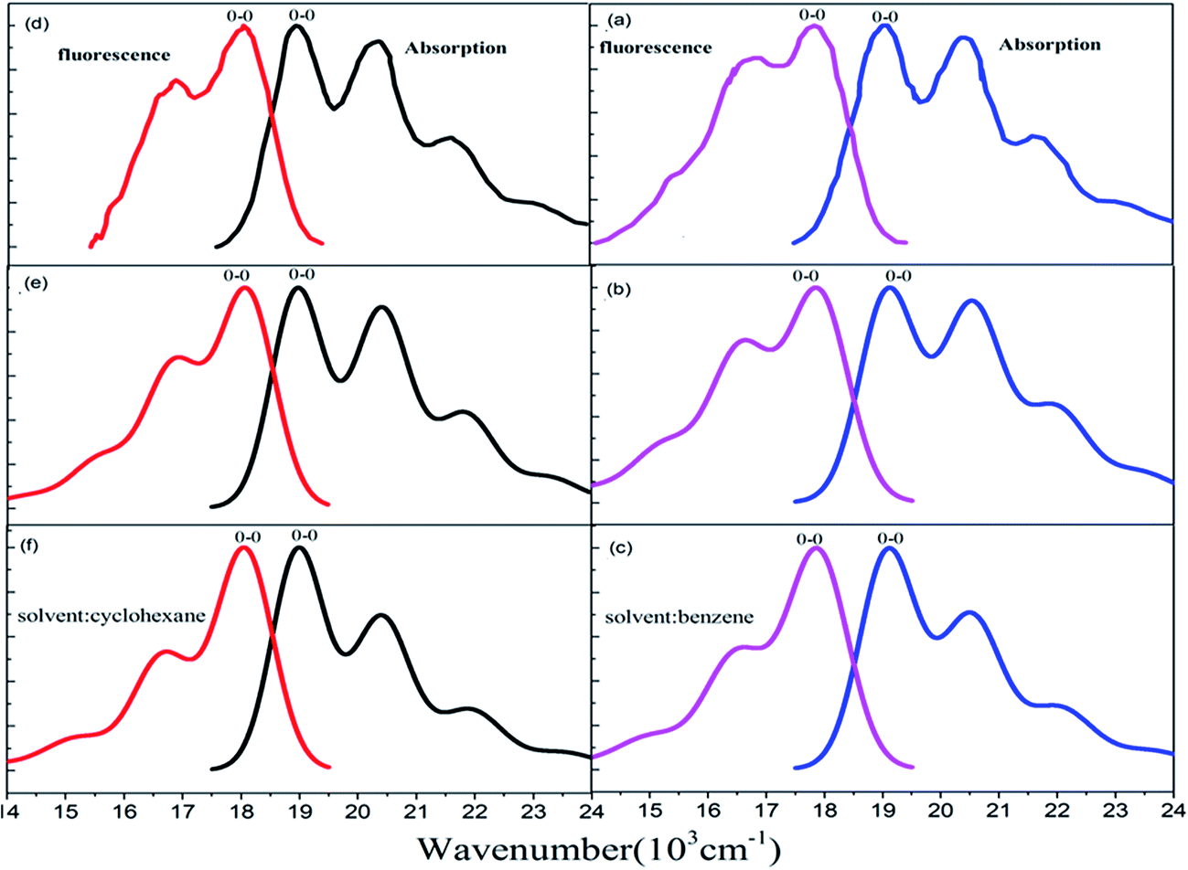
The Stokes shift (energy gap between the two peaks most close to adiabatic excitation energy ωba in absorption and fluorescence spectra) is 1120 cm−1, 1200 cm−1, and 1200 cm−1, respectively from experimental measurement (see Fig. 5(a)), and the present simulation with scaling (see Fig. 5(b)) and without scaling (see Fig. 5(c)) in benzene solvent. Actually, simulated vibronic band peaks all agree with experimental results as shown in Fig. 5, and the simulated peaks do not depend on change of scaling parameters as shown in Fig. S6 and S7 (ESI†). However, the intensity of the second maximum band peaks from simulation is much weaker than those from experiment for absorption spectrum if we compare Fig. 5(a) with Fig. 5(c), in fact, these solvent enhanced band shapes cannot be well reproduced without scaling. The first consideration about scaling is focused on all hydrogen atoms in rubrene as we did in ref. 36, however, there are distinct two group types of hydrogen atoms: one is 8 hydrogen atoms (15, 16, 17, 18, 23, 24, 25, and 26) on the backbone and the other is associated with four phenyl rings. The preliminary test was done by scaling all hydrogen atoms in the same way, and then we looked at how absorption spectrum varies as scaling parameters. We found there is little influence on spectrum by scaling those hydrogen atoms associated with four phenyl rings, while only scaling on 8 hydrogen atoms on the backbone makes sense of spectrum. This is actually consistent with analysis given in Subsection 3.1 about electronic excitation and molecular orbitals all related with the backbone atoms. Therefore, we work on only scaling 8 backbone-H atoms equally varying from ζH = 1.0, 1.4, 1.6, and 2.0 (no-scaling on the other hydrogen atoms and all carbon atoms), and we see from Table 4 that the only S values related to four active normal modes (ν15, ν16, ν17, and ν20) = (1389, 1416, 1555, and 1669) cm−1 change, while the rest of S values has no meaningful change. For instance, the S values change from 0.356, 0.050, 0.037, and 0.137 at ζH = 1.0 (means no scaling) to 0.069, 0.227, 0.288, and 0.247 at ζH = 2.0 for the corresponding four active normal modes (ν15, ν16, ν17, and ν20), respectively. Simulated absorption spectrum with scaling parameter at ζH = 2.0 well reproduces solvent enhanced absorption spectrum as shown in Fig. 5(b), besides the present scaling scheme is very smooth and stable (just like in ref. 36) as shown in Table 4 and S6 (ESI†) for absorption spectrum of rubrene molecule in benzene solvent.
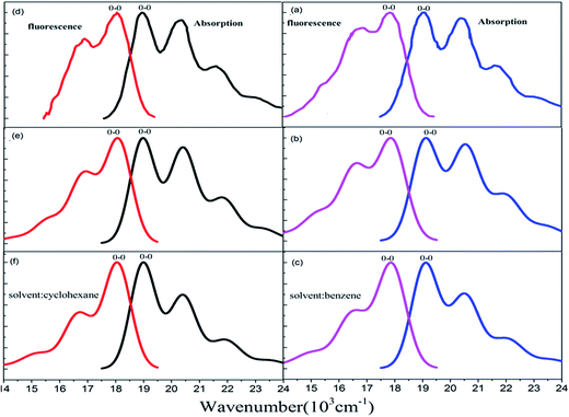 |
| | Fig. 5 Measured and calculated S0 (1Ag) → S1 (1B3u) absorption and S0 (1Ag) ← S1 (1B3u) fluorescence spectra at temperature T = 298 K. (a) Experiment from ref. 43, simulated (b) with and (c) without scaling in benzene solvent. (d) Experiment from ref. 42, simulated (e) with and (f) without scaling in cyclohexane solvent. | |
For fluorescence spectrum, we can see from Fig. 5(a) and (c) that intensity enhancement is not as much as absorption spectrum for the second maximum band peak and actually the present simulation works to some extent even without scaling. However, fluorescence band shape is not well reproduced without scaling. We have done the preliminary test with only scaling 8 backbone-H atoms, but it did not work out for detailed band shape. Therefore we add scaling on 12 carbon atoms (1, 2, 3, 4, 5, 6, 12, 13, 19, 20, 21 and 22) at two ends of the backbone, so that we make scaling on these 12 carbon atoms equally denoted as ζC= and on the 8 backbone-H atoms as ζH=, and the rest of H and C atoms are kept no scaling. In this way, simulated fluorescence spectrum with combination scaling ζH = 2.3 and ζC = 1.2 can reproduce detailed band shapes as shown in Fig. 5(b). We see from Table 5 that the only S values related to three active normal modes (ν13, ν14, and ν15) = (1384, 1423, and 1458) cm−1 change, and the rest of S values has no meaningful change. For example, the S values change from 0.182, 0.233, and 0.097 at ζH = 1.0 and ζC = 1.0 (means no scaling) to 0.0006, 0.315, and 0.491 at ζH = 2.3 and ζC = 1.2 for the corresponding three active normal modes (ν13, ν14, and ν15), respectively. Table 5 and Fig. S7 (ESI†) again show that the present scaling scheme is very smooth and stable for fluorescence spectrum of rubrene molecule in benzene solvent.
3.3. Absorption and fluorescence spectra in cyclohexane solvent
In cyclohexane solvent, the Stokes shift is 820 cm−1, 830 cm−1, and 830 cm−1, respectively from experimental measurement (see Fig. 5(d)), and the present simulation with scaling (see Fig. 5(e)) and without scaling (see Fig. 5(f)). Actually, all simulated peak positions in vibronic spectral bands agree with experimental results as shown in Fig. 5, and again simulated vibronic peaks do not depend on change of scaling parameters as shown in Fig. S8 and S9 (ESI†). For absorption spectrum in cyclohexane solvent, we work on only scaling 8 backbone-H atoms equally varying from ζH = 1.0, 1.4, 1.6, and 2.0 (like we did in benzene solvent), and we see from Table 6 that the only S values vary the almost same as those in Table 4 for four active normal modes (ν13, ν14, ν15, and ν17) = (1390, 1415, 1555, and 1669) cm−1. Simulated absorption spectrum with scaling parameter at ζH = 2.0 well reproduces solvent enhanced absorption spectrum in cyclohexane solvent as shown in Fig. 5(e).
For fluorescence spectrum in cyclohexane solvent, we do the same scaling as in benzene solvent for the 8 backbone-H atoms and 12 backbone-C atoms, and as a result, simulated fluorescence spectrum with combination ζH = 1.9 and ζC = 1.4 can well reproduce detailed band shapes as shown in Fig. 5(e). Table 7 shows that the only S values related to three active normal modes (ν12, ν14 and ν15) = (1286, 1384, and 1423) cm−1 change and the rest of S values has no meaningful change. Fig. S8 and S9 (ESI†) confirm that vibronic spectra vary very smoothly with respect to change of scaling parameters in cyclohexane solvent.
4. Concluding remark
We have employed four types of density functionals such as (TD)-B3LYP, (TD)-B3LYP35, (TD)-B3LYP50, and HF–CIS plus PCM models to investigate topology of potential energy surfaces on the ground state S0 and the first excited state S1 for rubrene. Geometry optimization calculations with the four-type functionals have revealed that there are four pairs of the local minima, S0-D2(1) and S1-D2(1), S0-D2(2) and S1-D2(2), S0-C2H(1) and S1-C2H(1), and S0-C2H(2) and S1-C2H(2), and one pair of the second-order transition state S0-D2H and S1-D2H that connect four local minima on S0 and S1 potential energy surfaces, respectively. The vibronic coupling distributions (Huang–Rhys factors) based on each pair of frequency calculations only support that the second-order transition state (S0-D2H and S1-D2H) can reproduce experimentally observed absorption and fluorescence spectra, and we have actually demonstrated that (TD)-BHandHLYP performs best for FC spectral simulation for rubrene molecule in benzene and cyclohexane solvents. The Stokes shift 1120 cm−1 (820 cm−1) and vibronic-band peak positions in absorption and fluorescence spectra in non-polar benzene (polar cyclohexane) solvent are well reproduced within the displaced harmonic oscillator FC simulation (no need to have damped correction). However, the second strongest vibronic-band peak intensities and shapes in both absorption and fluorescence spectra are not in good agreement with experiment results without the scaling, so that the damped FC simulation comes to apply to resolve this deviation. We found that only hydrogen atoms and carbon atoms associated with the aromatic backbone are sensitive to the scaling, while the hydrogen atoms and carbon atoms associated with four phenyl rings are not. Especially, we have shown in both absorption and fluorescence spectra that four vibrational modes around (1390, 1400, 1550, and 1670) cm−1 are responsible for solvent enhanced absorption spectra and three vibrational modes around (1290, 1380, and 1420) cm−1 are responsible for solvent enhanced fluorescence spectra. Those active modes all correspond to ring wagging plus CC stretch and CH bend motions of the atoms on the backbone, vibartional normal-mode motions associated with atoms on four phenyl rings are not active for vibronic spectra. Therefore, in the present work we have presented new physical insight how vibrational motions related to the aromatic backbone with D2H group symmetry play for interpreting solvent enhanced vibronic spectra of rubrene.
Acknowledgements
This work is supported by Ministry of Science and Technology of the Republic of China under grant no. 103-2113-M-009-007-MY3 and National Natural Science Foundation of P. R. China under grant no. 21673085. S.-H. L thanks supports from Ministry of Science and Technology of the Republic of China under grant no. 105-2923-M-009-003. Y. H. thanks support from visiting student fellowship by National Chiao Tung University. C. Z. thanks the MOE-ATU project of the National Chiao Tung University for support.
References
- S. H. Lin, C. H. Chang, K. K. Liang, R. Chang, Y. J. Shiu, J. M. Zhang, T. S. Yang, M. Hayashi, and F. C. Hsu, in Adv. Chem. Phys., John Wiley & Sons, Inc., 2002, pp. 1–88 Search PubMed.
- C. Zhu, K. K. Liang, M. Hayashi and S. H. Lin, Chem. Phys., 2009, 358, 137–146 CrossRef CAS.
- H. Hwang and P. J. Rossky, J. Phys. Chem. A, 2004, 108, 2607–2616 CrossRef CAS.
- P. Malmqvist and N. Forsberg, Chem. Phys., 1998, 228, 227–240 CrossRef CAS.
- F. T. Chau, J. M. D. Edmond, P. F. Lee and D. C. Wang, J. Electron Spectrosc. Relat. Phenom., 1998, 97, 33–47 CrossRef CAS.
- E. V. Doktorov, I. A. Malkin and V. I. Manko, J. Mol. Spectrosc., 1977, 64, 302–326 CrossRef.
- S.-Y. Lee, J. Phys. Chem., 1990, 94, 4420–4425 CrossRef CAS.
- H. Kikuchi, M. Kubo, N. Watanabe and H. Suzuki, J. Chem. Phys., 2003, 119, 729 CrossRef CAS.
- L. Yang, C. Zhu, J. Yu and S. H. Lin, Chem. Phys., 2012, 400, 126–136 CrossRef CAS.
- T.-W. Huang, L. Yang, C. Zhu and S. H. Lin, Chem. Phys. Lett., 2012, 541, 110–116 CrossRef CAS.
- T. Petrenko and F. Neese, J. Chem. Phys., 2007, 127, 164319 CrossRef PubMed.
- J. M. Luis, D. M. Bishop and B. Kirtman, J. Chem. Phys., 2004, 120, 813 CrossRef CAS PubMed.
- F. J. A. Ferrer, V. Barone, C. Cappelli and F. Santoro, J. Chem. Theory Comput., 2013, 9, 3597–3611 CrossRef PubMed.
- J. Lerme, Chem. Phys., 1990, 145, 67–88 CrossRef CAS.
- M. Roche, Chem. Phys. Lett., 1990, 168, 556–558 CrossRef CAS.
- A. Baiardi, J. Bloino and V. Barone, J. Chem. Theory Comput., 2013, 9, 4097–4115 CrossRef CAS PubMed.
- T. E. Sharp and H. M. Rosenstock, J. Chem. Phys., 1964, 41, 3453–3464 CrossRef CAS.
- H. Nagae, J. Chem. Phys., 1997, 106, 5159 CrossRef CAS.
- D. H. L. Linda and A. Peteanu, J. Phys. Chem., 1988, 92, 6554–6561 CrossRef.
- I. Baraldi, G. Brancolini, F. Momicchioli, G. Ponterini and D. Vanossi, Chem. Phys., 2003, 288, 309–325 CrossRef CAS.
- Y. H. Wang, M. Halik, C. K. Wang, S. R. Marder and Y. Luo, J. Chem. Phys., 2005, 123, 194311–194331 CrossRef PubMed.
- H. C. Georg, K. Coutinho and S. Canuto, J. Chem. Phys., 2007, 126, 034507–034510 CrossRef PubMed.
- I. F. Galvan, M. E. Martin, A. Munoz-Losa, M. L. Sanchez and M. A. Aguilar, J. Chem. Theory Comput., 2011, 7, 1850–1857 CrossRef PubMed.
- O. Clemens, M. Basters, M. Wild, S. Wilbrand, C. Reichert, M. Bauer, M. Springborg and G. Jung, J. Mol. Struct.: THEOCHEM, 2008, 866, 15–20 CrossRef CAS.
- J. Zeng, N. S. Hush and J. R. Reimers, J. Chem. Phys., 1993, 99, 1508 CrossRef CAS.
- T. Sakata, Y. Kawashima and H. Nakano, J. Chem. Phys., 2011, 134, 014501 CrossRef PubMed.
- O. V. Prezhdo, W. B. Valentyna, V. Zubkova and V. V. Prezhdo, J. Phys. Chem. A, 2008, 112, 13263–13266 CrossRef CAS PubMed.
- K. S. Schweizer and D. Chandler, J. Chem. Phys., 1983, 78, 4118–4125 CrossRef CAS.
- D. C. Tranca and A. A. Neufeld, J. Chem. Phys., 2009, 130, 141102 CrossRef CAS PubMed.
- A. N. Malakhov and A. L. Pankratov, in Adv. Chem. Phys., John Wiley & Sons, Inc., 2002, pp. 357–438 Search PubMed.
- H. J. Kim, J. Chem. Phys., 1996, 105, 6833 CrossRef CAS.
- Y. Shigemitsu, M. Uejima, T. Sato, K. Tanaka and Y. Tominaga, J. Phys. Chem. A, 2012, 116, 9100 CrossRef CAS PubMed.
- W. Y. So, J. Hong, J. J. Kim, G. A. Sherwood, K. Chacon-Madrid, J. H. Werner, A. P. Shreve, L. A. Peteanu and J. Wildeman, J. Phys. Chem. B, 2012, 116, 10504–10513 CrossRef CAS PubMed.
- F. Santoro, R. Improta, A. Lami, J. Bloino and V. Barone, J. Chem. Phys., 2007, 126, 084509 CrossRef PubMed.
- M. Dracinsky and P. Bour, J. Chem. Theory Comput., 2010, 6, 288–299 CrossRef CAS PubMed.
- C. W. Wang, L. Yang, C. Zhu, J. Yu and S. H. Lin, J. Chem. Phys., 2014, 141, 084106 CrossRef PubMed.
- H. Najafov, I. Biaggio, V. Podzorov, M. F. Calhoun and M. E. Gershenson, Phys. Rev. Lett., 2006, 96, 056604 CrossRef PubMed.
- N. Sai, M. L. Tiago, J. R. Chelikowsky and F. A. Reboredo, Phys. Rev. B: Condens. Matter Mater. Phys., 2008, 77, 161306 CrossRef.
- S. Tavazzi, A. Borghesi, A. Papagni, P. Spearman, L. Silvestri, A. Yassar, A. Camposeo, M. Polo and D. Pisignano, Phys. Rev. B: Condens. Matter Mater. Phys., 2007, 75, 245416 CrossRef.
- C. Udhardt, R. Forker, M. Gruenewald, Y. Watanabe, T. Yamada, T. Ueba, T. Munakata and T. Fritz, Thin Solid Films, 2016, 598, 271–275 CrossRef CAS.
- L. Carmichael and G. L. Hug, Radiat. Phys. Chem., 1985, 26, 229–246 CrossRef.
- T. Petrenko, O. Krylova, F. Neese and M. Sokolowski, New J. Phys., 2009, 11, 015001 CrossRef.
- S. Tavazzi, L. Silvestri, M. Campione, A. Borghesi, A. Papagni, P. Spearman, A. Yassar, A. Camposeo and D. Pisignano, J. Appl. Phys., 2007, 102, 023107 CrossRef.
- S. Chang, N. B. Rex and R. K. Chang, J. Opt. Soc. Am. B, 1999, 16, 1224–1235 CrossRef CAS.
- G. M. Badger and R. S. Pearce, Spectrochim. Acta, 1951, 4, 280–288 CrossRef CAS.
- F. Gao, W. Z. Liang and Y. Zhao, J. Phys. Chem. A, 2009, 113, 12847 CrossRef CAS PubMed.
- A. D. Becke, Phys. Rev. A, 1988, 38, 3098–3100 CrossRef CAS.
- H. C. Corben and P. Stehle, Classical Mechanics, Dover Publication, Inc., New York, 2nd edn, 1994 Search PubMed.
- M. J. Frisch, G. W. Trucks and H. B. Schlegel, Gaussian 09, Revision C.01, Gaussian, Inc., Wallingford, CT, 2010 Search PubMed.
- Q. Peng, Y. Yi, Z. Shuai and J. Shao, J. Am. Chem. Soc., 2007, 129, 9333 CrossRef CAS PubMed.
Footnotes |
| † Electronic supplementary information (ESI) available. See DOI: 10.1039/c7ra00417f |
| ‡ Y. Hu and C.-W. Chen contributed equally to this work. |
|
| This journal is © The Royal Society of Chemistry 2017 |
Click here to see how this site uses Cookies. View our privacy policy here. 
 Open Access Article
 This Open Access Article is licensed under a
  *ab,
Fenglong Gu*a and
Sheng-Hsien Linb
*ab,
Fenglong Gu*a and
Sheng-Hsien Linb

 is the average phonon distribution, γba is the homogeneous broadening parameter and Dba is inhomogeneous broadening parameter that reflects static interaction between electronic states of molecule and solvent, and ωj is the j-th normal mode vibrational frequency. The dimensionless Huang–Rhys factor Sj corresponding to the j-th normal mode is defined as

 and qn in eqn (4) are the mass-weighted Cartesian coordinates at equilibrium geometries (or transition states) of the electronic excited and ground states, respectively. Transformation matrix L in eqn (4) can be computed with frequency analysis using G09 programs, for instance. By applying damped diatomic harmonic oscillator to local-mode force constant of gas-phase Hessian matrix Hij, we formulate damped FC factors as transferring the mass-weighted gas-phase unperturbed Hessian matrix to solvent perturbed Hessian matrix,36
 is converted to perturbed force constant
 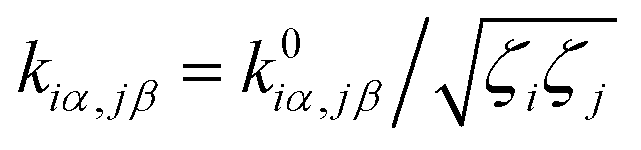 . The dimensionless scaling parameter ζj in eqn (5) is treated as an empirical parameter that can be considered as a local dynamic interaction of atom j of solute molecule with solvent molecules. By diagonalizing perturbed Hessian matrix in eqn (5), we obtain normal mode frequencies and transformation matrix (that transfers the mass-weighted Cartesian coordinates to normal mode coordinates) corresponding to solute molecule under the solvent environment. It should be emphasized that solvent effect by damped oscillator can directly modify the leading-term of FC factors, so that it is usually larger than the other effects such as distorted oscillator, Duschinsky effect and anharmonic effect which are in higher-order perturbation terms.