DOI:
10.1039/C6RA28615A
(Paper)
RSC Adv., 2017,
7, 12764-12774
Experimental study and transient CFD/DEM simulation in a fluidized bed based on different drag models
Received
23rd December 2016
, Accepted 6th February 2017
First published on 23rd February 2017
Abstract
Gas–solid two-phase flow is the main phenomena in the chemical-looping combustion (CLC) fluidized bed system. Drag force generated from relative movement between phases is the main force that hinders the movement of the oxygen carrier particles. It is important to evaluate and understand the limitations and validity range of different drag models. In this paper, based on Discrete Elements Methods (DEM) coupled with Computational Fluid Dynamics (CFD), three kinds of drag models, Wen-Yu, Syamal-O'Brien, and Gidaspow, are used for the simulation of a laboratory-scale spouted fluidized bed. The numerical results based on these three models are compared and analyzed from the views of the bed height, bubble diameter, and pressure fluctuations. A spouted fluidized bed experiment rig was established to carry out the high-speed imaging experiment and validate the numerical results. All three drag models could basically describe the transient behavior of the bubble shape. In the first stage of whole fluidization process, Syamal-O'Brien drag model could predict well both the change of the bubble diameter and the bubble shape in good agreement with experiment results, but the model for the bubble collapse status is not a good prediction; Wen-Yu drag model underestimates the variations in bubble diameter and predicts the occurrence of the next fluidization stage prematurely; although, the Gidaspow drag model still slightly underestimates the change of bubble diameter, but the results of this drag model are in good agreement with the experiment results in terms of the bubble shape, and pressure fluctuations. Under the architecture of CFD/DEM, the Gidaspow drag model gives the better prediction of the inner flow in the dense gas–solid fluidized bed. The results provide reference for the further improved design of the fluidized bed by employing the CFD/DEM method.
1. Introduction
Reducing carbon emissions from fossil-fueled power plants has been an active area of research in recent years. One technology that appears to be very promising for high-efficiency low-cost carbon capture is chemical-looping combustion (CLC). CLC involves combustion of fuels (either gas or solid) by heterogeneous chemical reactions with an oxygen carrier, usually a particulate metal oxide. Gas–solid two-phase flow is the main phenomena in a CLC fluidized bed.1 It is important and difficult to study the characteristics of the gas–solid two-phase flow for further improved design of the fluidized bed, especially for the condition of high solid concentration.2
Over decades, many researchers carried out plenty of laboratory-scale fluidized bed experiments to explore the characteristics of the flow inside the fluidized beds, such as the minimum fluidization velocity, the bed height, and particle aggregation, etc. There are many kinds of classifications of particles, however, the generally accepted method is the one summarized by Geldart,3 which is based on a huge number of experimental results. Among them, Geldart D particles are those with large diameter and high density. These particles are widely used in experimental studies because they can obviously present an aggregation state during fluidization process. However, restricted by the present experimental level, it is hard to obtain microscopic kinetic information during collision by experiment.
With the development of computer technology and parallel computing, numerical simulation has become the primary means of studying the inner flow characteristics of the fluidized bed. Currently, there are two main methods for the numerical simulation of gas–solid two-phase flows:4 the first is the Euler–Euler method, also known as the Two-Fluid Model (TFM) which is based on the classical hydrodynamics theory. In this method, each phase is considered as a continuum and specifies the particle amount in the mixture of two phases by the particle volume fraction, and employs the constitutive equations of the granular theory to calculate the inter-particle forces. This model costs less computer facility and computational time-consuming, it mainly used in high mass loading situations and reaction occasions which focus on the energy exchange during reaction processes, such as the simulation of chemical-looping pilot plant5 and the simulation of chemical-looping combustion reactor with chemical reactions.6 The second approach is the Euler–Lagrange method, which regards the fluid phase as a continuum and the solid particles as the discrete phase. Then the continuity equation for the fluid phase and the Newtonian equations for the discrete phase are solved using the force-balance method to obtain the discrete phase trajectories. Compared to the Euler–Lagrange method, the main disadvantage of Euler–Euler method is that this method does not take into account the properties of the particles, such as Young's modulus, elastic modulus, particle diameter, etc., and also ignores the collision between the particles and the particles-walls.7 Discrete Elements Methods (DEM) belongs to the deterministic model of the Euler–Lagrange method, which is able to describe the translational and rotational motion of the particles by calculating the Newtonian equations. It also considers the collisions among the particles and the particles-walls. As a result, this model is widely used for calculating the dense gas–solid two-phase flow of solid phase volume fraction greater than 12%. According to the particles kinetic theory, particles will suspend in the bed when the forces exerted from the fluid phase equal gravity.
In describing the hydrodynamics of gas–solid flow systems, drag force which is exerted by the fluid phase is one of the main contributing factors. Different scholars based on numerous experiment results had established a variety of drag models. Until now, there are mainly three drag models are used to calculate the gas–solid flow in a fluidized bed, which are Syamal-O'Brien model, Wen-Yu model and Gidaspow model. Owing to the relatively complicated experiment situations and inner flow characteristics, there are still no clear guidance in choosing the appropriate drag model for different experiment situations. Many researches used Two-Fluid Model (TFM) to simulate the gas–solid two phase flow. Lu et al.8 developed a new non-spherical particle drag model based on TFM to simulate the supercritical water fluidized bed. These simulation results were validated by comparing with experimental data and the bed expansions agreed well with experimentally measured data. Askaripour et al.9 conducted the 3D modeling and simulation of bubbling fluidized beds using various drag models based on TFM. They explored a wide range of solid size, static bed height and results of expansion ratio and solids velocity were compared with experimental data. It was found that Wen-Yu drag model provided the best prediction of expansion ratio and solids velocity. Wang et al.10 proposed a new drag model based on TFM which incorporated the contribution of meso-scale structure effects for Geldart-B particles, the simulation results obtained by the new model showed better agreement with the experimental results than Gidaspow model. However, it is also apparently that these simulation results obtained by TFM contained considerable deviations, so Euler–Lagrange model gets more attention recently. Ayeni et al.11 analyzed the inadequacies of the traditional drag laws in predicting pressure drop and velocity, and proposed a new drag law based on energy and force balance in fluidized bed which took into account additional energy for heterogeneous structure. And this model enforced the macroscopic conservation principles while attempting to still accommodate local variations in drag due to cluster formation mechanisms.
Until now, the investigations of drag models used in dense gas–solid two phase flow are insufficient, especially for the Euler–Lagrange method. In this paper, by coupling the CFD and DEM, we investigated three most commonly used drag models to discuss their applicability and defect in dense gas–solid two phase flow. The inner-flow characteristics, such as the bed height, bubble diameter, particle velocity distribution and pressure fluctuations are compared among these different drag models. Furthermore, these prediction results are compared with the high-speed imaging experimental results, which could serve as references for the further application and improvement of drag models.
2. Mathematical modeling
2.1 Mass and momentum balances
DEM can be considered as a kind of soft sphere model, which considers the particle penetration depth and volume fraction of discrete phase and continuous phase in infinitesimal calculating element simultaneously.
Let εg denote the porosity; the motion of the fluid phase obeys the laws of governing mass and momentum conservation equations and that can be written as:12,13
| |
 | (1) |
| |
 | (2) |
where
ρg is the gas density,
ug is the velocity vector,
p is the static pressure,

is the stress tensor,
g is the gravitational acceleration, and
FDEM is the external force generated by all the moving particles which acts on the infinitesimal fluid element (
e.g. the force generated due to interaction of the fluid phase with the discrete phase). Conservation of mass and momentum of fluid phase can also be applied in dispersed phase.
Considering that the existence of a pressure field is a necessary condition, when solving the Navier–Stokes equations of the fluid phase, the pressure field and the velocity field must be coupled via the continuity equation. Thus the SIMPLE algorithm in ANSYS-Fluent 16.0 is employed to ensure this coupling. Furthermore, for high solid concentration fluidized bed, the standard k–ε turbulence model is employed to simulate the turbulent flow in the reactor; it is satisfactory since the more complex turbulence models such as the full Reynolds Stress Model (RSM) or Large Eddy Simulation (LES) are computationally complex and expensive with limited benefit in accuracy of the simulations.14
The motion of particles in a fluidized bed are mainly moving and rotating. The equations of particle movement and rotation are:
| |
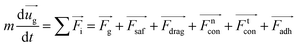 | (3) |
| |
 | (4) |
where
m is the mass of the particle,
ug is the particle velocity and
Fi is the sum of various forces acting on the particle including gravity, Saffman force, drag force, short range force and the adhesive forces. Specifically, the adhesive forces contain either with or without physical contact. The adhesive forces with physical contact are based on the formation of a physical bond between particles or particles and wall, such as solid bridges. The adhesive forces without physical contact include van der Waals and electrostatic forces.
2.2 Discrete element method
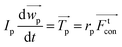
There are plenty of forces that can cause particles moving, among which the most important farces are gravity, drag force and short-range forces. In this paper, elastic-damper model15,16 is used to calculate the short-range forces during particle collision. In the discrete element method, it is assumed that the particles can overlap each other and penetrate into the wall. Then the particle–particle collision force is calculated by the penetration depth. Similar procedures can be used to calculate the contact force due to the particle-wall collision with the assumptions that the wall has an infinite radius. This model includes Hooke's elastic model and Newton's damping model. The elastic model is used for modelling the reversible deformation, while the damping model for irreversible and time-dependent deformation. The torque acting on a particle resulting from the tangential contact force and causing the particle to rotate can be calculated by multiplying the tangential contact force with the particle radius. Fig. 1 shows a brief introduction of the model, and, in the figure, the part A and B are the normal and tangential collision models between particles, part C and D are the normal and tangential collision models between particle and wall.
 |
| | Fig. 1 A simplified linear elastic model in the collision process. | |
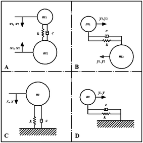
When evaluating the collisions between parcels, it is too costly to conduct a direct force evaluation that involves all of the parcels. Consider that for N parcels, the number of pairs that would need to be inspected for every time step would be on the order of N2. To address this issue, as shown in Fig. 2, a geometric approach is used: the domain is divided by a suitable Cartesian mesh (where the edge length of the mesh cells is a multiple of the largest parcel diameter), and then the force evaluation is only conducted for parcels that are in neighboring mesh cells, because particles in more remote cells of the collision mesh are a priori known to be out of reach.12
 |
| | Fig. 2 Force evaluation for parcels.12,13 | |
What should be mentioned here is that the simulation results will contain a certain error if the particle size is larger than the fluid cell size. Generally, there are two strategies being most commonly used to deal with the problem of particle size. The first method is using relatively large fluid cell size which is 2.5 to 3 times of the particle size. This method is most commonly used in many occasions because it increases the computational velocity. The other strategy takes the inter-phase coupling into consideration to modify calculation resolution. This strategy includes the porous media concept and the two-grid concept. For the porous media concept, it regard the flow field as a porous media. The porous media model can be used for a wide variety of single phase and multiphase problems, including flow through packed beds, filter papers, perforated plates, flow distributors, and tube banks.17 For the two-grid concept, the physical values of the fluid and solid phases are determined in separated grids, namely the fluid and article grids. The fluid physical variables obtained in a fine fluid grid are transferred to the coarse particle cells to calculate the inter-phase momentum and energy exchange.18
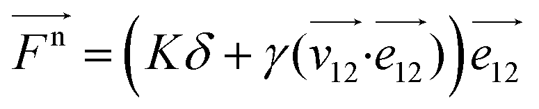
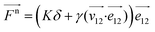
Let K be the elastic collision coefficient and η (0 < η ≤ 1) be the damper restitution coefficient, thus the formula of the Spring–Dashpot Collision Law are as follows:
| |
 | (5) |
| | |
δ = ||X2 − X1|| − (r1 + r2)
| (6) |
where
X1 and
X2 are the locations of particle 1 and 2,
r1 and
r2 are the radius of 1 and 2,
δ is the penetration depth of particle–particle and particles-wall.
| |
 | (7) |
| |
 | (8) |
| |
 | (9) |
| |
 | (10) |
| |
 | (11) |
| |
 | (12) |
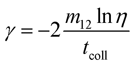
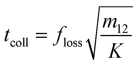
where
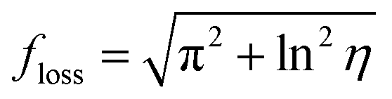
floss is a loss factor,
m1 and
m2 are the mass of particle 1 and 2;
m12 is the mass loss in the collision process;
tcoll is the collision time scale;
v1 and
v2 are the velocity of particle 1 and 2;
v12 is the relative velocity;
γ is the damping coefficient.
12
2.3 Drag model
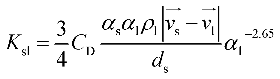
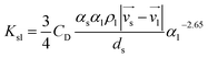
Momentum exchange between phases is mainly according to the momentum exchange coefficient Ksl, which is the most different feature between these three models.
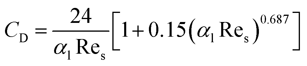
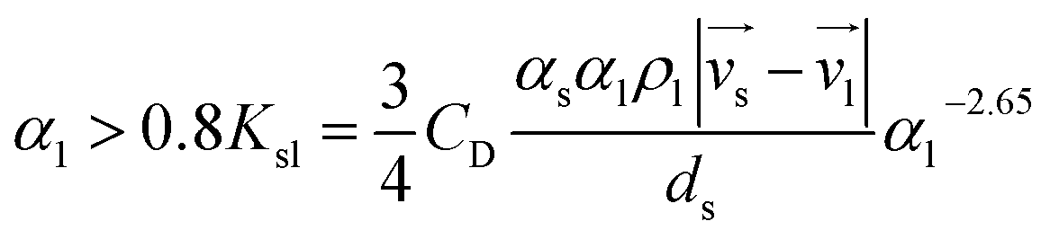
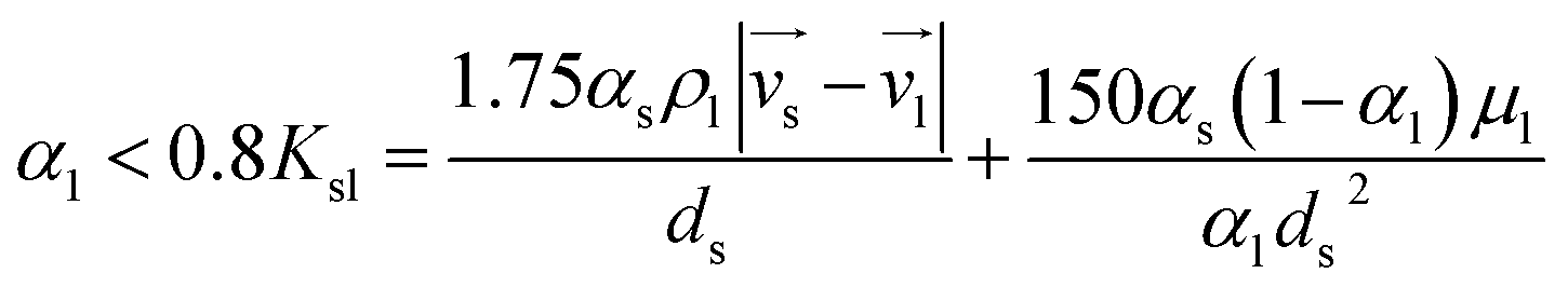
2.3.2 Gidaspw drag model. Gidaspw drag model combines Wun-Yu model and Ergun model, which takes discrete phase proportion into consideration. This model is suitable for particulate systems where viscous forces are dominant, for example dilute flows.20 Let αl be the porosity of continuous phase. When αl is greater than 0.8, Wen-Yu is chosen, on the contrary, when αl is under 0.8 Ergun model is selected. Therefore, the formula of Gidaspw model is as follows:| |
 | (16) |
| |
 | (17) |
where CD is the drag coefficient:| |
 | (18) |
As can be seen from these formulas, when αl is under 0.8, the drag model is unrelated to the Reynolds number. However, when αl is greater than 0.8, the value of CD follows the change of Reynolds number.
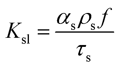
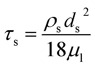
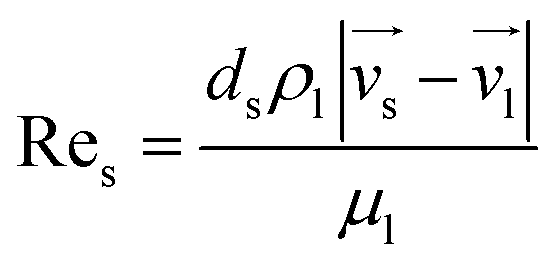
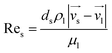
2.3.3 Syamal-O'Brien drag model. The Syamal-O'Brien drag model is based on the notion that for single- and multi-particle systems the Archimedes number remains the same for terminal setting velocity.21The momentum exchange coefficient between phases is:
| |
 | (19) |
| |
 | (20) |
where
τs is particle relaxation time,
ds is particle diameter,
μl is viscosity of fluid phase.
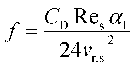
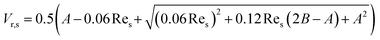
f is a function of the drag coefficient CD and Reynolds number Re. The model is based on the terminal velocity Vr,s of the particle phase in the fluid field, volume fraction α and the corresponding particle phase Reynolds number Res. The formula is:
| |
 | (21) |
where
| |
 | (22) |
So the momentum exchange coefficient of Syamal-O'Brien drag model is:
| |
 | (23) |
where particle terminal velocity and Reynolds number are:
| |
 | (24) |
| |
 | (25) |
where
A =
αl4.14 and
B = 0.8
αl1.28 (
αl ≤ 0.85),
B =
αl2.65 (
αl > 0.85).
3. Experimental and numerical methods
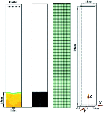
As shown in Fig. 3, a spouted fluidized bed experimental rig was set up in the Fluid Machinery Laboratory, Jiangsu University. The quasi-3D fluidized bed is made of plexiglass, with the length, width and height of 15 cm, 2 cm, and 100 cm, respectively. The selected solid particles are consisted of 30![[thin space (1/6-em)]](https://www.rsc.org/images/entities/char_2009.gif) 000 average diameter of 2.5 mm glass beads. The initial bed height is about 15 cm, which is measured by the ruler embedded in the right side of the bed. The air is supplied through a centrally placed nozzle at the inlet. Inlet low rate of 300 L min−1 at room temperature is carried out in the experiment, which is controlled by a high accuracy mass flow controller. Pressure fluctuations in the bed are measured by three pressure sensors located at the height of 2 cm, 22 cm, and 40 cm, respectively. The particle aggregation and dispersion in the fluidized bed are taken in real time by a high speed camera placed in front of the bed.
000 average diameter of 2.5 mm glass beads. The initial bed height is about 15 cm, which is measured by the ruler embedded in the right side of the bed. The air is supplied through a centrally placed nozzle at the inlet. Inlet low rate of 300 L min−1 at room temperature is carried out in the experiment, which is controlled by a high accuracy mass flow controller. Pressure fluctuations in the bed are measured by three pressure sensors located at the height of 2 cm, 22 cm, and 40 cm, respectively. The particle aggregation and dispersion in the fluidized bed are taken in real time by a high speed camera placed in front of the bed.
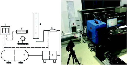 |
| | Fig. 3 Test rig for the fluidized bed experiment (1. Computer 2. High speed camera 3. Light 4. Fluidized bed 5. Mass flow controller 6. Refrigeration dryer 7. Air compressor). | |
As shown in Fig. 4, in order to explore the internal mechanism of the flow of the fluidized bed, a 3D solid model was established in full agreement with the experimental geometry. At the bottom of the fluidized bed piled up 30000 of 2.5 mm diameter spherical particles, programmatically. At first, we conduct a series of air-blowing and free-fall simulation to achieve the randomness of the initial particle packing, which is called the starting point (t = 0). For DEM simulation, since the gas phase equation and the momentum exchange coefficient are both based on the volume of the control body, when establishing the mesh model, the diameter of the mesh must be larger than the diameter of the particle.22–25 On this basis, through the grid independence analysis, determine the total number of grid as 22880, and the number of grid nodes in the length, width and height are 22, 4 and 260, respectively. Inlet is set as mass flow inlet and outlet is set as pressure outlet. The motion of fluid phase is modeled by using the standard k–ε turbulence model, and Spring–Dashpot26,27 model is used to solve the collision process between particles and particles-walls. The setting parameters are listed in Table 1.
 |
| | Fig. 4 Computational model of the fluidized bed. | |
Table 1 DEM Simulation Parameters
| Parameters |
Value or Setting |
| Avg. diam. of particles |
2.5 mm |
| Avg. density of particles |
2500 kg m−3 |
| Total number of particles |
30000 |
| Gas inlet velocity |
300 L min−1 |
| Restitution coefficient in normal direction (P–P, P–W) |
0.97 |
| Restitution coefficient in tangential direction (P–P, P–W) |
0.33 |
| Spring constant |
410 kN m−1 |
| Drag law |
Gidspow, Wun-Yu, Syamal-O'Brien |
| Under relaxation velocity |
0.3 |
| Under relaxation pressure |
0.2 |
| Numerical schemes |
Phase coupled SIMPLE |
| Time step size of particle phase |
2.5 × 10⁻⁵ s |
| Time step size of gas phase |
1 × 10⁻⁵ s |
4. Results and discussions
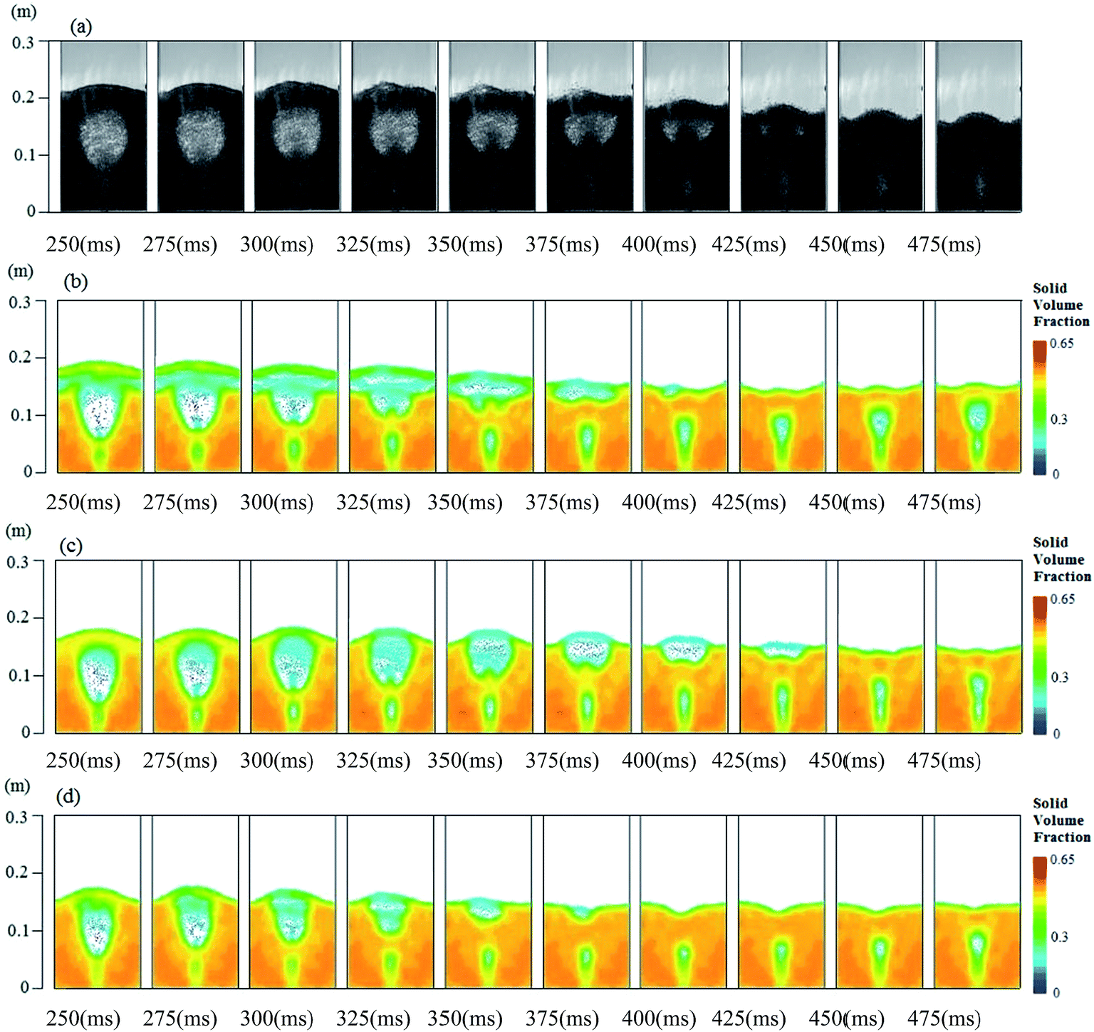
4.1 Transient bubble shape comparison
As shown in Fig. 5, (a) is the experimental high-speed imaging results, while (b)–(d) are simulation results of these three drag models, respectively. The latter three pictures represent the volume fraction of particle–phase distribution along Z orientation, which all under the same range from 0 to 0.7. At t = 0, all these three cases have the same stacking height, about 15 cm. Obviously, there is a slight difference of initial bed height between numerical simulation and experiment, which is mainly due to that 4.1 × 10⁵ N m−1 is chosen as the linear-elastic collision coefficient between particles according to experience when using DEM model for calculation. If this value is bigger, the deformation during collision is smaller, and vice versa. Through the analysis of enormous simulation and experimental results, it can be found that this value is reasonable because, in the DEM model, the selection of the value is consistent with the allowed mutual penetration depth of the model and the calculation accuracy is also considered. During the previous 75 ms period, these calculation results of three drag model are in good agreement with experimental results. With the further development of fluidized state, the bed height becomes higher and the bubble area grows, while particles at the top of the bubble moving towards both sides of the bed so that the upper portion of the bed becomes increasingly sparse, where these three drag force models can be well observed. During 100 ms to 225 ms time period, Syamal-O'brien model slightly overestimates the size of the bubble, in contrast, Gidaspow model slightly underestimated the size of the bubble and Wen-Yu model underestimates the size of the cavity. As bubble size is directly related to the drag force generated by the relative motion between phases, the smaller drag force, the smaller bubble diameter is, and vice versa.
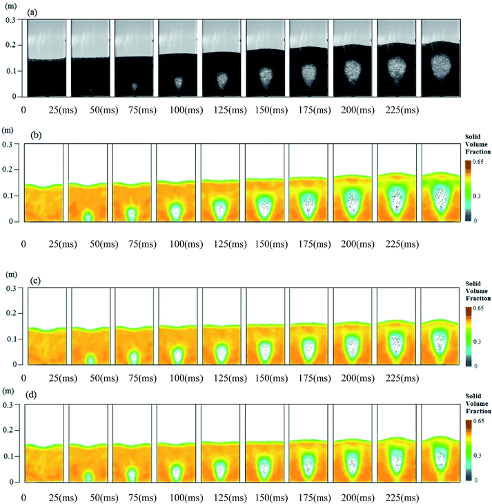 |
| | Fig. 5 Comparison of experimental and numerical results from 0 to 225 ms with 300 L min−1 inlet velocity ((a) experimental results, (b) Syamal-O'Brien model, (c) Gidaspow model, (d) Wen-Yu model). | |
Fig. 6 is shown for the comparison of high-speed imaging experimental results and numerical simulation results from 250 ms to 475 ms time period. With the increasing of the bubble volume, the velocity of upper particles moving to both sides of the walls increases, leading to the particle layer on the top of the bed becomes much sparser and the gap between the particles is gradually increased. At the time when the internal pressure of the bubble is greater than the surface pressure of the bed, the air escape from the gap between particles to the outlet. During a gas overflow process, the particles on the top of the bubble ejected into the free area till the bubble finally burst, showing an extremely unstable fluidized state. The upper thickness of the bubble of all these three drag model are relatively small, while Syamal-O'brien model cannot well describe the bubble rupture process, representing that the performance of the gas within the bubble cannot get through the top layer of the bed showing an slugging fluidized state. Wen-Yu model is too early to predict the flow of the next fluidized stage process, performing that the bed collapses prematurely and also the bubble area is relatively small. But, Gidaspow model can well predict the vacuoles rupture process, bed collapse process and the bubble shape.
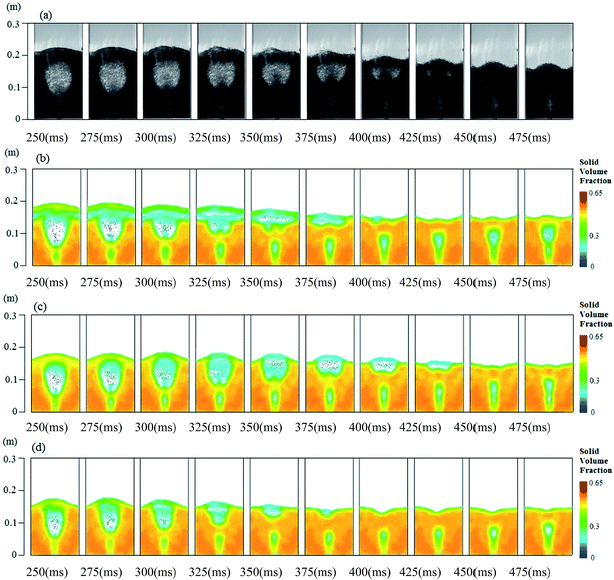 |
| | Fig. 6 Comparison of experimental and numerical results from 250 to 475 ms with 300 L min−1 inlet velocity ((a) experimental results, (b) Syamal-O'Brien model, (c) Gidaspow model, (d) Wen-Yu model). | |
4.2 Fluidization characteristics
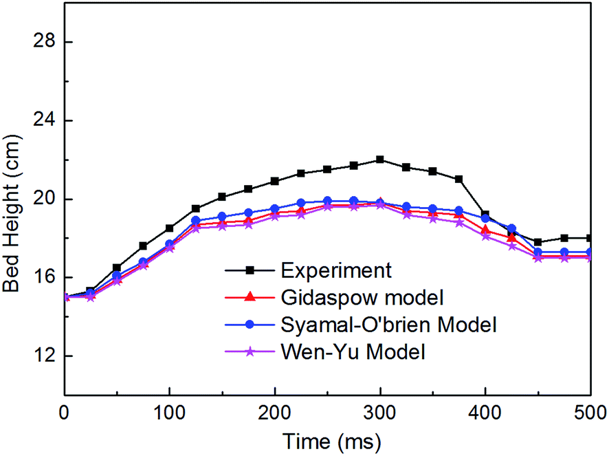
Fig. 7 shows the comparison of the bed height of all these three different drag models. Obviously, the bed height, along with the time, shows the process of rise and fall, and peaks at around 300 ms. At the stage of nearly completely slump, the initial bed height was significantly higher than the initial bed height, this is because, after the gas entering into the bed, the gas fills in the gaps between the particles, and because of the continuous influx of gas kept at the inlet leading to a lifted state of the fluidized bed. Within the initial 125 ms, these three kinds of drag model can well describe the changes of the bed height, however, differences began to appear at around 125 ms, and from 125 ms to 400 ms period, all these three kinds of drag model are significantly undervalued the changes of the bed height, which is probably due to the fact that in order to guarantee the initial accumulation state of the bed in simulation is consistent with the experiment as much as possible, there is a subsidence at the middle. This is resulted from, during the simulation process, the underlying particles rise with bubble expending to compensate for the height difference. Meanwhile, due to the interphase momentum exchange is severe in the expanding section of the bed, as a result, the relatively small force, such as particle non-contact stress, becomes much larger in a short time, while these forces are often ignored in the simulation.
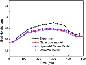 |
| | Fig. 7 Comparison of bed height between the experiment and simulation of the three drag models. | |
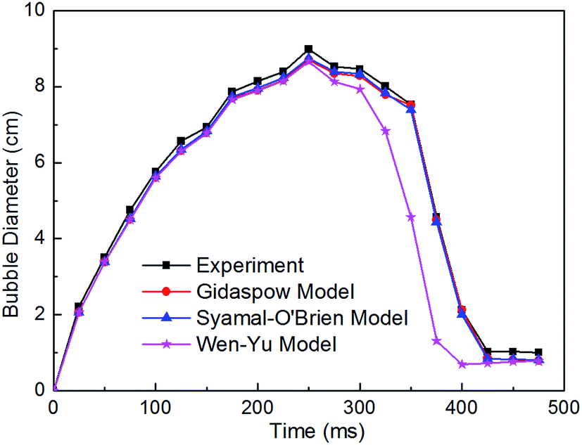
Fig. 8 shows the contrast of the bubble diameter between experimental results and numerical simulation results. The size of the bubble diameter is an important benchmark to measure the performance of the internal flow of a spouting fluidized bed. To quantify the scale size of bubble, the bubble diameter is defined as:
| |
 | (26) |
where
Ab represents the area of the bubble which is measured by a professional drawing software.
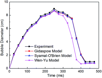 |
| | Fig. 8 Comparison of bubble diameter between the experiment and simulation of the three drag models. | |
It is apparent from the figure that the simulation results of the three drag model from 0 to 250 ms time period coincide with the experimental results quite well, and the bubble diameter peaks at 250 ms. With the further development of fluidized state, Wen-Yu models significantly underestimated the changes of the bubble diameter, meanwhile, the model predict the changing time into the next fluidization stage is too earlier. However, the other two models have good prediction about the changes of the bubble diameter.
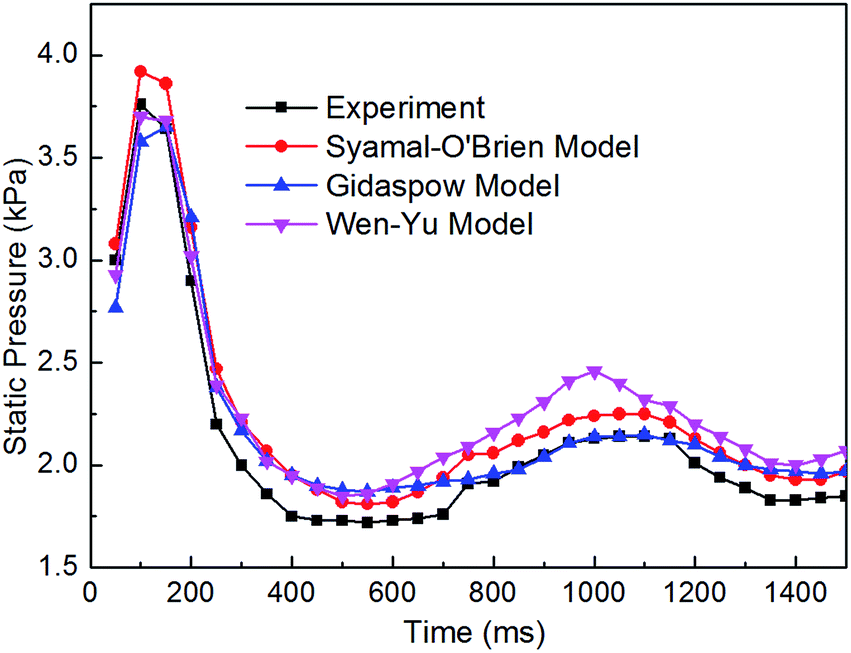
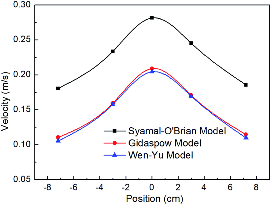
As shown in Fig. 9, these are the static pressure fluctuations at the monitoring point of x = 7.5 cm, y = 0 cm, z = 2 cm. We could find that all these three models can well predict the pressure fluctuations at that point, showing that the trend of all the pressure fluctuations are consistent and the maximum velocity appears in the vicinity of 150 ms. The bed rises rapidly in this period and interphase momentum exchange is intense. However, with the fluidized state grows further, the pressure prediction of Syamal-O'brien model is significantly higher than the other two models and experimental values, Gidaspow model can well describe pressure fluctuations comparatively. Fig. 10 shows the velocity distribution profile at z = 10 cm, along the y-axis, of all these three kinds of drag models. It can be seen that the velocity is symmetric distribution along the Y–Z plane. The simulation results of Gidaspow model and Wen-Yu model is similar but significantly lower than the Syamal-O'brien model. This is probably due to that the calculation of drag force on the Syamal-O'brien model is based on the terminal velocity of the particles, when the volume fraction is less than 0.85, the calculated terminal velocity of particle phase is relatively low, while the next fluidization stage is ready to happen at this period, so the bed fluctuation is significant, leading to the calculated drag force is much higher.
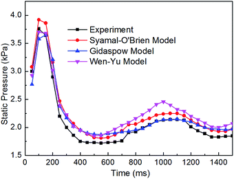 |
| | Fig. 9 Comparison of pressure fluctuations between the experiment and simulation of the three drag models. | |
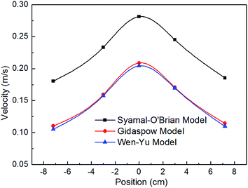 |
| | Fig. 10 Comparison of velocity at Z orientation between the simulation of the three drag models at t = 150 ms. | |
5. Discussions
Fig. 11 compares the particle velocity predicted by three drag models at t = 250 ms. For the above differences in the simulation of a three-dimensional bubbling fluidized among these drag models and experimental results, it can probably be that Syamal-O'brien model is calculated based on the relative velocity coefficient model and the huge number of experimental data and summed up by Richardson and Zaki, so this model can be used to simulate the relatively dense two-phase flow systems. Meanwhile this model assumes that the Archimedes number of a single particle is the same as that of the all the particles in the entire system. The difference between simulation result and experimental result at the initial stage of the fluidization process can be that in this stage forced convection plays a leading role so the Archimedes number of a single particle and particles throughout the flow field is close. But when the bed is in a transport state, free convection also occupies a certain proportion, which means that in this state the Archimedes number of particles is not all the same, so there is some differences between experimental result and simulation result of the bubble ruptured state.
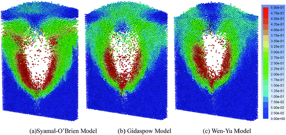 |
| | Fig. 11 3D snaps of particle velocity magnitude (m s−1) predicted by three drag models at t = 250 ms. | |
Gidaspow model integrates Wen-Yu model and Ergun model based on the principle that internal forces between particles are negligible, which means that viscous forces dominate the two-phase flow system, so this model is suitable for relatively dilute gas–solid two phase systems. For the difference between simulation results and experimental results it can be that, in this bubbling fluidized bed, a particle diameter is relatively large, about 2.5 mm, thus, compared to the viscous force, the impact force between particles is also the main force. Still, when the gas-phase volume fraction is greater than 0.8, the Wen-Yu model is chosen, and the gas-phase volume fraction is less than 0.8, the Ergun model is chosen. While the bubble under approaches to rupture, the gas phase volume fraction, which is in the vicinity of 0.8, changes significantly, thereby computing model switched more frequently, resulting in some errors with data transmission method and the accuracy is not good enough. In addition, for typical applications, the computational cost of tracking all of the particles individually is prohibitive. Instead, the approach for the discrete element method is similar to that of the DPM, in that like particles are divided into parcels, and then the position of each parcel is determined by tracking a single representative particle. During the fluidization process, the particles are not in the presence of a single particle, but gathering together in the form of particle groups. Considering the number of the particles used in this simulation, the simplification that leading to the underestimate of the agglomeration force is relatively large, so using this model to calculate the overall system makes the particle distribution more uniform and leads to a certain deviations. At the same time, when calculating the interaction forces between particles, there are many physical parameters (such as elastic modulus, coefficient of restitution etc.) of the particle phase is unknown, but is often determined by the experience, which will inevitably result in some errors.
The key difference between these three drag models is the drag coefficient CD. For Wen-Yu and Gidaspow drag model, the former model is the complement and extension of the latter model, and Gidaspow drag model takes low porosity of continuous phase into consideration, so it is more accurate. For Gidaspow drag model and Syamal-O'brien drag model, it is the different drag coefficient that results in the differences between the two simulation results. Syamal-O'brien drag model considers particle terminal setting velocity which based on the assumption that the Archimedes number is the same for the velocity, but it cannot well predict the bubble rupture stage because at this stage free convection plays a significant role which means that the Archimedes number is not the same. Overall, it is more accurate to use the Gidaspow drag model than the Syamal-O'brien drag model to simulate the gas–solid flow in this spouted fluidized bed.
6. Conclusions
This paper using different drag models to carry out the exploration of the application CFD/DEM. Syamal-O'brien model, Gidaspow model and Wen-Yu model were selected for the simulation of gas–solid flow in a spouted fluidized bed. A high-speed imaging experiment rig was established to compare and validate the numerical predicted results. It could be found that these three models can well predict the movement trend of the particle phase in the fluidized bed, but the simulated bed height were significantly underestimated compared to the experiment result. However, in terms of the changes of the bubble diameter, Gidaspow model and Syamal-O'brien model are good predictors of these changes. In general, the simulation results of Gidaspow model are in good agreement with experimental results. As for the small differences, it is mainly because that when the fluidized bed is in a transportation state, free convection plays a certain role, so the Archimedes number of all the particles in the bed is different, however the model assumes that the Archimedes number of a single particle is the same as that of the whole.
However, since many physical parameters are not clear when using the DEM model to calculate the particle phase, there are some differences between experimental results and simulation results in the calculation of particle collision and bubble ruptured state. But it can be found from these data, the error is within 2.5% for the simulation using Gidaspow drag model, which can be considered that Gidaspow drag model is appropriate apply in the simulation of the dense gas–solid fluidized bed. Meanwhile, there remains to be much work to seek or establish an improved drag model to predict the bubble rupture process and the latter process with more precision.
Acknowledgements
This work was supported by the National Natural Science Foundation of China (Grant No. 51609106), Natural Science Foundation of Jiangsu Province (Grant No. BK20150508), Jiangsu Province Universities Natural Sciences Foundation (Grant No. 15KJB570001), and the funding for the Construction of Dominant Disciplines in Colleges and Universities and Universities in Jiangsu (PAPD).
References
- T. Ogada and J. Werther, Combustion characteristics of wet sludge in a fluidized bed: release and combustion of the volatiles, Fuel, 1996, 75(5), 617–626 CrossRef CAS.
- J. Zhu and J. Hong, Development and present situation of the jet bed, Chem. React. Eng. Technol., 1997, 2, 207–230 Search PubMed.
- D. Geldart, Types of gas fluidization, Powder Technol., 1973, 7(5), 285–292 CrossRef CAS.
- W. P. Adamczyk, G. Węcel and M. Klajny, et al., Modeling of particle transport and combustion phenomena in a large-scale circulating fluidized bed boiler using a hybrid Euler–Lagrange approach, Particuology, 2014, 16(5), 129–140 CrossRef.
- F. Alobaid, P. Ohlemüller and J. Ströhle, et al., Extended Euler–Euler model for the simulation of a 1 MWth, chemical–looping pilot plant, Energy, 2015, 93, 2395–2405 CrossRef CAS.
- S. Banerjee and R. K. Agarwal, An Eulerian approach to Computational Fluid Dynamics simulation of a Chemical-Looping Combustion reactor with chemical reactions, J. Phys. Chem. B, 2015, 110(10), 4756–4765 Search PubMed.
- W. P. Adamczyk, A. Klimanek and R. A. Białecki, et al., Comparison of the standard Euler–Euler and hybrid Euler–Lagrange approaches for modeling particle transport in a pilot-scale circulating fluidized bed, Particuology, 2014, 15(4), 129–137 CrossRef.
- Y. Lu, L. Wei and J. Wei, A numerical study of bed expansion in supercritical water fluidized bed with a non-spherical particle drag model, Chem. Eng. Res. Des., 2015, 104, 164–173 CrossRef CAS.
- H. Askaripour and A. M. Dehkordi, Simulation of 3D freely bubbling gas–solid fluidized beds using various drag models: TFM approach, Chem. Eng. Res. Des., 2015, 100, 377–390 CrossRef CAS.
- Y. Wang, Z. Zou and H. Li, et al., A new drag model for TFM simulation of gas–solid bubbling fluidized beds with Geldart-B particles, Particuology, 2014, 15, 151–159 CrossRef.
- O. O. Ayeni, C. L. Wu and K. Nandakumar, et al., Development and validation of a new drag law using mechanical energy balance approach for DEM–CFD simulation of gas–solid fluidized bed, Chem. Eng. J., 2016, 302, 395–405 CrossRef CAS.
- Ansys Inc., Ansys Fluent theory guide, Ansys Inc., Southpointe 275 Technology Drive, Canonsburg, PA, 2015a, p. 15317 Search PubMed.
- Ansys Inc., Asnys Fluent therory guide, Release 16.0, Ansys Inc., Canonsburg, PA, USA, 2015b Search PubMed.
- S. Benzarti, H. Mhiri and H. Bournot, Drag models for simulation gas–solid flow in the bubbling fluidized bed of FCC particles, World Academy of Science, Engineering and Technology, 2012, 61, 1138–1143 Search PubMed.
- Y. Tsuji, T. Kawaguchi and T. Tanaka, Discrete particle simulation of two-dimensional fluidized bed, Powder Technol., 1993, 77(1), 79–87 CrossRef CAS.
- J. F. Dietiker, T. Li and R. Garg, et al., Cartesian grid simulations of gas–solids flow systems with complex geometry, Powder Technol., 2013, 235(2), 696–705 CrossRef CAS.
- V. S. Sutkar, N. G. Deen, V. Salikov, S. Antonyuk, S. Heinrich and J. A. M. Kuipers, Experimental and numerical investigations of a pseudo-2D spout fluidized bed with draft plates, Powder Technol., 2015, 270, 537–547 CrossRef CAS.
- F. Alobaid, A particle-grid method for Euler–Lagrange approach, Powder Technol., 2015, 286, 342–360 CrossRef CAS.
- F. Vejahati, N. Mahinpey and N. Ellis, et al., CFD simulation of gas–solid bubbling fluidized bed: a new method for adjusting drag law, Can. J. Chem. Eng., 2009, 87(1), 19–30 CrossRef CAS.
- W. Sobieski, Switch function and sphericity coefficient in the Gidaspow drag model for modeling solid–fluid systems, Drying Technol., 2009, 27(2), 267–280 CrossRef.
- S. Zimmermann and F. Taghipour, CFD modeling of the hydrodynamics and reaction kinetics of FCC fluidized-bed reactors, Ind. Eng. Chem. Res., 2005, 44(26), 9818–9827 CrossRef CAS.
- Y. Guo, C. Y. Wu and C. Thornton, Modeling gas-particle two-phase flows with complex and moving boundaries using DEM–CFD with an
immersed boundary method, AIChE J., 2013, 59(4), 1075–1087 CrossRef CAS.
- Y. Q. Zhuang, X. M. Chen and Z. H. Luo, et al., CFD–DEM modeling of gas–solid flow and catalytic MTO reaction in a fluidized bed reactor, Comput. Chem. Eng., 2014, 60, 1–16 CrossRef CAS.
- Z. Zhang, Z. Ling and R. Agarwal, Transient Simulations of Spouted Fluidized Bed for Coal-Direct Chemical Looping Combustion, Energy Fuels, 2014, 28(2), 1548–1560 CrossRef CAS.
- E. Esmaili and N. Mahinpey, Adjustment of drag coefficient correlations in two dimensional CFD simulation of gas–solid bubbling fluidized bed, Advances in Engineering Software, 2011, 42(6), 375–386 CrossRef.
- S. Gerber, F. Behrendt and M. Oevermann, An Eulerian modeling approach of wood gasification in a bubbling fluidized bed reactor using char as bed material, Fuel, 2010, 89(10), 2903–2917 CrossRef CAS.
- N. Almohammed, F. Alobaid and M. Breuer, et al., A comparative study on the influence of the gas flow rate on the hydrodynamics of a gas–solid spouted fluidized bed using Euler–Euler and Euler–Lagrange/DEM models, Powder Technol., 2014, 264(3), 343–364 CrossRef CAS.
|
| This journal is © The Royal Society of Chemistry 2017 |
Click here to see how this site uses Cookies. View our privacy policy here. 
 Open Access Article
 This Open Access Article is licensed under a Creative Commons Attribution-Non Commercial 3.0 Unported Licence
 *ab,
Lingjie Zhanga,
Ling Baia,
Weidong Shia,
Wei Lia,
Chuan Wang*a and
Ramesh Agarwalb
*ab,
Lingjie Zhanga,
Ling Baia,
Weidong Shia,
Wei Lia,
Chuan Wang*a and
Ramesh Agarwalb


 is the stress tensor, g is the gravitational acceleration, and FDEM is the external force generated by all the moving particles which acts on the infinitesimal fluid element (e.g. the force generated due to interaction of the fluid phase with the discrete phase). Conservation of mass and momentum of fluid phase can also be applied in dispersed phase.