Enhanced phase and amplitude image contrasts of polymers in bimodal atomic force microscopy

Abstract

Bimodal atomic force microscopy (AFM), where the first two flexural eigenmodes of the cantilever are simultaneously excited, is an extension of dynamic AFM to enhance the contrast of multicomponent materials. The effects of the operating parameters for both modes are explored by imaging a polymer blend of polystyrene (PS) and low-density polyethylene (LDPE) the in attractive and repulsive regimes. In this study, the phase and amplitude contrasts of the individual eigenmodes for bimodal AFM are quantitatively calculated using a statistical expression. Meaningfully, the higher free amplitudes of the second mode, which were chosen beyond the traditional values, show significantly better compositional contrast, particularly for the phase of the second mode. The phase contrast of the second mode increases by 3–10 times compared with that of the traditional results. The relationship between the contrast and amplitude ratio of the first mode is also researched experimentally in the bimodal mode. Virial and energy dissipation power for the corresponding modes are employed to explain the enhanced phase contrast physically. The meaningful results obtained are applicable to optimize the operating parameters of image contrast and study the surface morphology and properties of soft, even biological materials.

---

1. Introduction

Multiple frequency atomic force microscopy (MF-AFM) is a promising branch of AFM where the cantilever is driven and measured at two or more frequencies.^1–4 As the most typical use, Rodriguez and Garcia proved the ability of bimodal atomic force microscopy in enhancing the resolution and sensitivity of compositional materials in 2004.⁵ In bimodal AFM, the cantilever is excited by the first and second flexural resonance frequencies simultaneously. Two lock-in amplifiers are used to detect and demodulate the mixed signals with respect to the first and second resonance frequencies. The amplitude of the first mode, which provides the topography information of the sample surface, is kept constant by the feedback control system at a fixed setpoint during scanning. However, the amplitude and phase of the second mode are set free to reflect the changes in the mechanical, magnetic or electrical properties of the sample surface.⁶

Usually, the excitation frequencies of bimodal AFM are tuned to match the first two resonances. The cantilever of the rectangular beam is always approximately modeled by the Euler–Bernoulli partial differential equation to describe the dynamics of the cantilever-tip system. Similarly, two differential equations are assumed for the dynamics of the bimodal system.⁶

where i stands for the eigenmode; k_i, ω_i = 2πf_i, and Q_i are the modal stiffness, resonance frequency, and Q factor of the i mode, respectively. F_0i = k_iA_0i/Q_i is the magnitude of the i mode external driving force. F_ts is the tip-sample interaction. A_0i and z_i are the free amplitude and deflection of the cantilever for mode i, respectively. When the tip-sample non-linear interaction works, the response of the cantilever in the bimodal mode can be approached by the following equation:

z(t) = z₀ + z₁(t) + z₂(t) + O(ε) ≈ A₁ cos(ω₁t − Ø₁) + A₂ cos(ω₂t − Ø₂) (2)

where z₀ is the mean deflection, A_i is the amplitude and Ø_i is the phase shift of the i eigenmode. O(ε) is a term that carries the contribution of the other modes and harmonics. Based on these equations, we can choose different excited functions to obtain the amplitudes and phase shifts of the response channels of the i modes. Amplitude and phase are main signals used to distinguish materials and interaction types (i.e., conservative versus dissipation).⁷ Previous experiments and theoretical simulations have shown that the higher mode is more sensitive to material variations.^8–10 Herruzo et al. simultaneously mapped the Young's modulus and viscous and damping coefficients of soft matter surfaces with nanoscale spatial resolution.¹¹ Martinez et al. resolved the structural components of antibodies in both monomer and pentameric forms by operating bimodal experiments in air and liquid.¹² Proksch showed that bimodal frequency excitation produces a variety of frequency dependent sample properties for graphite, which can be related to its electronic properties.¹³ In particular, polymers¹⁴ and soft biological samples, such as DNA,¹⁵ polystyrene,¹⁶ protein¹⁷ and phospholipids, need a low force to enhance their compositional contrast. In most bimodal works, the free amplitude of the second mode (several nanometers) is about one order of magnitude smaller than the first free amplitude. The argument is that the higher magnitude of the second mode may affect the first mode vibration. For this nonlinear interaction system, virial and dissipated power were employed to plot the relative dominance of the conservative and non-conservation (dissipative) tip-sample interactions.^18–20 Energy transfer or changes between the two modes might reveal the origin of the contrast.²¹

In the present study, we characterize a polymer blend in attractive and repulsive regimes via bimodal atomic force microscopy. The amplitude setpoint of the first mode is 0.7 for all three free amplitudes. The free amplitude of the second mode varies from 1 nm to 60 nm by gradual intervals, which includes lower and higher driving amplitudes for the free higher mode channels. Both the energy dissipation power and virial of the conservative tip-surface forces may carry coupling information for the excited modes; thus in this study, they are explored to establish the relationship between the free amplitude and compositional contrast of two AFM mode images. Different regimes are divided to express the reverse of the amplitude and phase between the PS and LDPE regions, which are closely related to the change in the tip-sample interaction. Furthermore, we quantify the contrast for all the phase and amplitude images to compare and optimize the operation parameters. Results show that higher free amplitudes of the second mode correspond to more energy dissipation power and virial values. Similarly, the higher the energy dissipation power and virial, the better the compositional contrast. In the large free amplitudes regime for the second mode, the phase contrast is much better than that obtained from the other two response channels, which might have future applications in soft materials. Finally, the dependencies between the contrast and amplitude setpoint ratio of the first mode are researched when the second mode free amplitude is fixed. This can also illustrate that there is energy transfer between the two modes associated with free amplitude and setpoint ratio.

2. Experimental

Bimodal imaging experiments were performed using a commercial Cypher AFM setup (Asylum Research, Santa Barbara, CA) equipped with wide bandwidth circuit and high frequency cantilever holders. A polymer blend of polystyrene (PS) and low density polyethylene (LDPE), which was purchased from Bruker Nano Inc., was used to obtain high contrast in the phase signals. Circular domains (LDPE) were mixed in the substrate (PS matrix). The inverse optical lever sensitivities (also called InvOLS, which is a parameter necessary for the spring constant algorithm) were calibrated from dynamic amplitude approaching curves on a freshly cleaved mica surface for the first flexural mode and the second flexural mode. Based on the equipartition theorem, the spring constants were calculated by fitting the thermal data captured from the thermal noise power spectra method.^22,23 Moreover, the flexural resonance frequencies and quality factors of the first and second modes were determined. Calibrating AC160 cantilever by this method, the first and second flexural resonance frequencies of the cantilever are f₁ = 344.246 kHz and f₂ = 1.939 MHz; the first and the second mode dynamic spring constants are k₁ = 42.44 N m⁻¹ and k₂ = 918.46 N m⁻¹; the quality factors of the two modes are Q₁ = 353.6 and Q₂ = 553.7, respectively.

The sinusoidal voltage signal was used to drive the base of the cantilever with a piezo stack in conventional amplitude modulated AFM, where the amplitude was kept constant at a user-defined setpoint by the feedback control circuit. Different unconstrained free amplitudes of the first flexural mode A₀₁ (54, 40 and 25 nm) were chosen, and the ambient amplitude setpoint ratio was 0.7 (for a single AM-AFM cycle away from the surface, the phase lag/offset is always set to 90 degrees. With a change in distance between the tip and sample, the amplitude and phase also change. If the phase shift is positive, it is customary to refer to the imaging mode as “attractive”. If the phase shift is negative, the mode is referred to as “repulsive”).

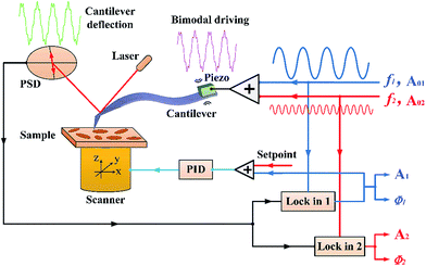
Compared to first single mode tuned in conventional AM-AFM, the driving frequencies of the two modes should be tuned exactly to the first and second flexural resonance frequencies before bimodal imaging experiments. Therefore, a linear combination of two sinusoidal voltages was applied to drive the cantilever during the bimodal imaging experiments. The first amplitude was kept constant by the feedback system as in the case of monomodal AM-AFM. The second amplitude and phase were not constrained by any feedback mechanism. The free amplitude of the first flexural mode was A₀₁, which varied from 54, 40 and 25 nm. During the experiment process, the free amplitude of the second flexural mode A₀₂ increased gradually. We also comparatively researched material contrast at different free amplitudes of the second mode. The dependencies between the contrast and amplitude setpoint ratio of the first mode were also researched when the second mode free amplitude was set to 20 nm. The controlling scheme of bimodal imaging in the Cypher AFM setup is shown in Fig. 1.

Fig. 1 Controlling scheme of bimodal imaging in the Cypher AFM setup.

3. Results and discussion

3.1. Amplitude and phase of bimodal mode

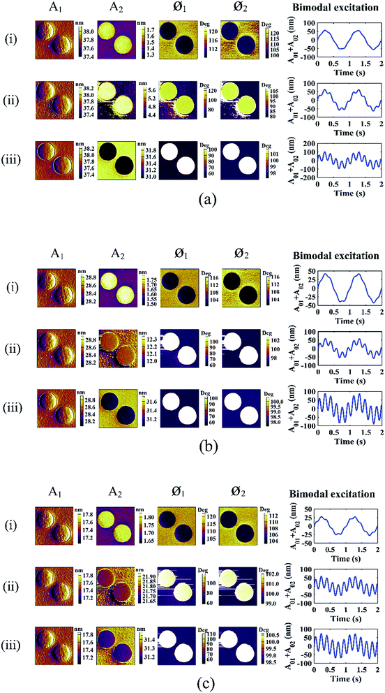
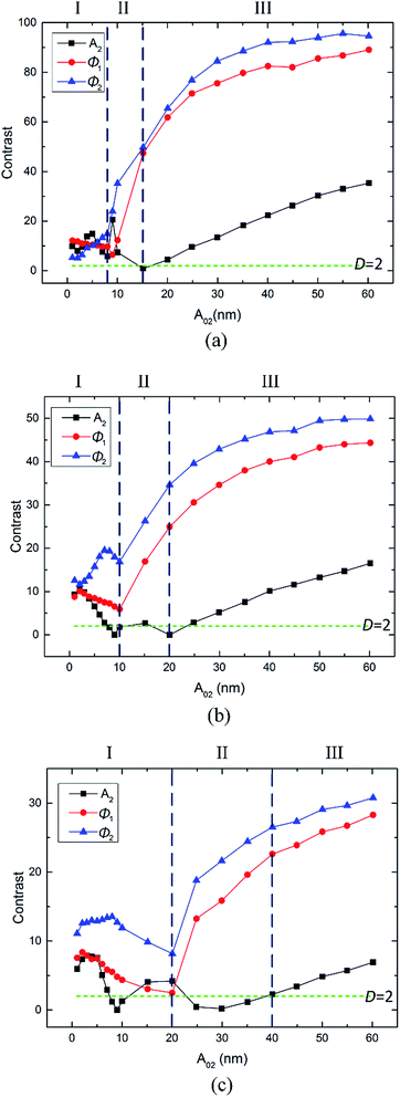
Bimodal imaging experiments were carried out by exciting the AC160 cantilever. The free amplitudes of the first flexural mode A₀₁ were maintained at 54, 40 and 25 nm, respectively. The free amplitude of the first flexural mode is a crucial parameter that may influence the interaction regime between the tip and sample. The free amplitude of the second mode A₀₂ varied sequentially in a small interval over the course of the specific free amplitude A₀₁. Unlike previously reported, a wide range of values of A₀₂ was used to explore more information on material contrast. The setpoint ratio of the first flexural mode was about 0.7, which might ensure imaging from attractive to repulsive regimes. The second mode scanning amplitude A₂, the first mode phase Ø₁ and the second mode phase Ø₂ images obtained during the scanning are shown in Fig. 2.

Fig. 2 2.5 × 2.5 micrometer AFM signals of PS-LDPE imaged by an Olympus AC160 cantilever in the bimodal AFM mode. Free amplitudes (a) A₀₁ = 54 nm, (b) A₀₁ = 40 nm and (c) A₀₁ = 25 nm. (i) A₀₂ = 2.94 nm, (ii) transitional A₀₂ and (iii) A₀₂ = 50 nm are the three chosen values of the second mode free amplitudes performed in the respective A₀₁. The amplitude and phase images are in nm and degrees, respectively.

Fig. 2 shows the bimodal excitations and scanning amplitude A₁, scanning amplitude A₂, phase Ø₁ and phase Ø₂ images obtained in the bimodal experiments. Fig. 2(a)–(c) display images with different free amplitudes A₀₁ (A₀₁ = 54, 40 and 25 nm). The rows in Fig. 2(i)–(iii) represent the free amplitudes A₀₂ (2.94 nm, transitional value and 50 nm, respectively). The transitional value (in the contrast reversal range) of the free amplitudes A₀₂ are 10, 20 and 35 nm for the different free amplitudes A₀₁ = 54, 40 and 25 nm. For amplitude A₁, no color difference can be found except the bright edges around the LDPE regions, which may be caused by the topography variation. Therefore, the contrast of A₁ is rather low because of the feedback mechanism. As the free amplitude of the second mode A₀₂ increases, the contrast of PS-LDPE reverses into three stages. In the first stage, the amplitude A₂ image is bright in the LDPE regions, and phase Ø₁ and phase Ø₂ display a dark color at a small free amplitude A₀₂. As A₀₂ increases to the second stage, reversal of the phase Ø₁ and phase Ø₂ images arises between the PS and LDPE regions and the amplitude A₂ images are still bright in the LDPE regions. With A₀₂ increasing further, the image contrast of amplitude A₂ reverses, which is the third stage. Therefore, there are two reversal points throughout the course of varying the A₀₂ values in experiments. One is the reversal point in the phase (Ø₁ and Ø₂) image series and the other is the reversal point in the amplitude A₂ image series.

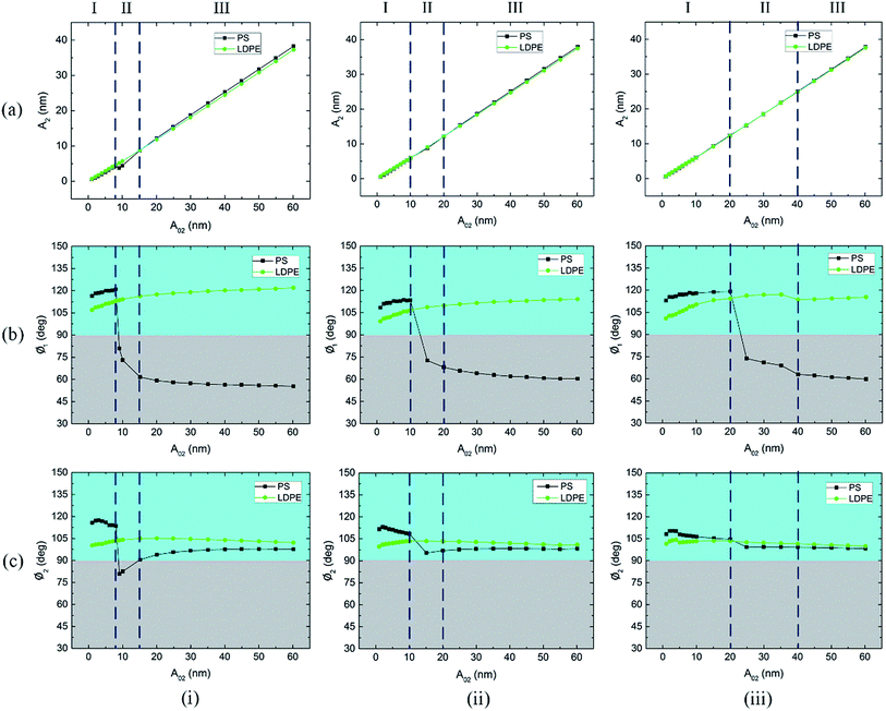
The second mode free amplitude A₀₂ gradually increased throughout the course of the experiments when the other parameters remained constant. Fig. 3(a)–(c) summarize the changes in the amplitude A₂, phase Ø₁ and phase Ø₂ average values in the PS and LDPE regions with different free amplitudes A₀₂. The rows in Fig. 3(i)–(iii) represent free amplitude A₀₁ = 54, 40 and 25 nm, respectively. According to the aforementioned two reversal points, three regimes I, II and III are divided in Fig. 3.

Fig. 3 The three free amplitudes are columns (i) A₀₁ = 54 nm, (ii) A₀₁ = 40 nm and (iii) A₀₁ = 25 nm. (a) Amplitude A₂, (b) phase Ø₁ and (c) phase Ø₂ are summarized with different A₀₂. Three regimes I, II and III are divided in every image set. The amplitude and the phase images are in nm and degrees, respectively.

The average scanning amplitude A₂ versus free amplitude A₀₂ in Fig. 3(a) shows a good linear relationship. In regime I and II of Fig. 3(a), the A₂ values in the LDPE regions are a little bigger than those in the PS regions, whereas in regime III, the A₂ values in the LDPE regions become smaller than those in the PS regions. This also illustrates the reversal of A₂ image contrast between the PS and LDPE regions. In regime I of Fig. 3(b), the Ø₁ values in the PS regions are bigger than those in the LDPE regions. Moreover, all these values are larger than 90 degrees in regime I. In regime II and III of Fig. 3(b), the phase in the LDPE region remains stable, similar to that in regime I. However, it falls below 90 degrees and remains stable in regime III. In regime I of Fig. 3(c), the Ø₂ values in the PS regions are larger than those in the LDPE regions. In regime II and III, the phase in the LDPE region also remains stable, but falls in regime II and remains stable in regime III in the PS region. Differently, the Ø₂ values of both PS and LDPE regions are almost larger than 90 degrees in all the regimes. The reversal point of phase (Ø₁ and Ø₂) contrast between the PS and LDPE regions is clear. Generally, regime II is a transition period corresponding to unstable images and poor contrast. At the same time, regime II becomes wider and moves to the right (greater A₀₂) when the free amplitude A₀₁ becomes smaller.

3.2. Dissipation

Energy-based quantities (dissipated power and virial), which carry information on phase and amplitude, can be used to describe the conservative and dissipative interactions between the tip and the sample.^24,25 Phase contrast is closely connected to the magnitude of the dynamic energy dissipation per vibrating cycle as the cantilever scans the sample in the AM-AFM mode. Similarly, the energy dissipation for each mode is calculated and discussed in this study. Another key definition associated with the phase and amplitude signals is virial, which carries information on conservative tip-sample forces. The average power dissipated, P_dis(i), and virial, V_i, for the ith mode per cycle are calculated using the following analytical expressions:^26,27where f_i is the ith mode free resonance frequency, A_0i is the ith mode free amplitude, A_i is the ith mode scanning amplitude, k_i is the ith mode dynamic spring constant, Q_i is the ith mode quality factor, and Ø_i is the ith mode phase.

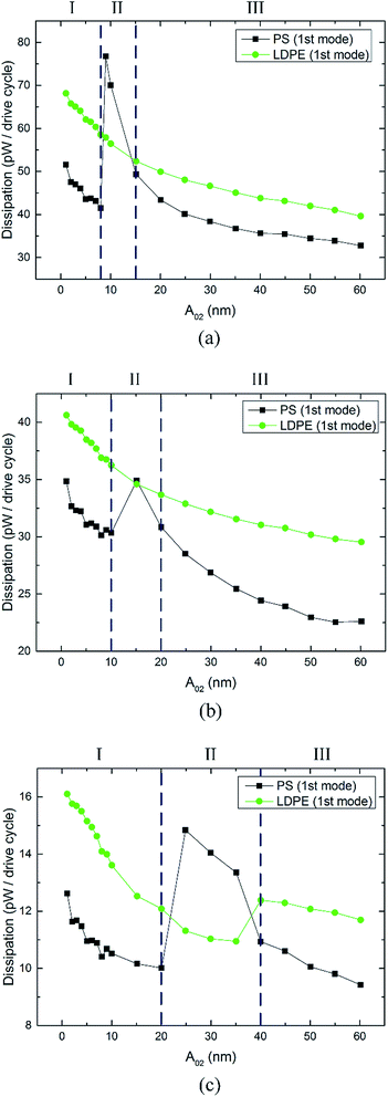
Fig. 4 shows the energy dissipation curves of the first mode measured on PS-LPDE with varying free amplitudes A₀₂. Fig. 4(a)–(c) are plotted with different free amplitudes A₀₁ = 54 nm, A₀₁ = 40 nm and A₀₁ = 25 nm, respectively. Regimes I, II, and III are divided by the deep blue dot lines on the basis of two reversal points. In Fig. 4(a), the energy dissipation in the LDPE region shows a gentle downward trend (from 68 to 40 pW) when the free amplitudes A₀₂ increase from 1 to 60 nm. The energy dissipation in the PS region is lower than that in the LDPE region in regime I and III. Moreover, the energy dissipation curve shows a flat downward trend in regime I and III. However, it suddenly jumps from 41 to 77 pW in regime II, which reveals a disorder phenomenon corresponding to unstable image and poor contrast. In Fig. 4(b) and (c), the energy dissipation on both components presents a similar regular trend. Significantly, they show less energy dissipation for a smaller free amplitude A₀₁.

Fig. 4 Energy dissipation curves of the first mode measured on PS-LPDE with varying free amplitudes A₀₂. Free amplitude (a) A₀₁ = 54 nm, (b) A₀₁ = 40 nm and (c) A₀₁ = 25 nm. Regimes I, II and III are divided by the deep blue dot lines on the basis of the contrast reversal points.

Fig. 5 shows the second mode energy dissipation curves (hollow points) measured on PS-LDPE by varying the second mode free amplitudes A₀₂. Fig. 5(a)–(c) display energy dissipation versus different free amplitudes A₀₁ (54, 40 and 25 nm). In Fig. 5(a), the relationship between A₀₂ and energy dissipation has the shape of half a parabola. The numerical values of the energy dissipation for different A₀₂ increase from 2 to 8261 pW per vibrating cycle. The partially enlarged detail in Fig. 5(a) shows a cross point of the second mode energy dissipation in the PS and LDPE regions, which is consistent with the phase reversal point of the second mode. The first mode dissipation P_dis(1) and second mode dissipation P_dis(2) are approximately equal when A₀₂ = 5 nm. Clearly, the dissipation of the first mode and second mode are in the same order of magnitude when A₀₂ is below 10 nm. When it is greater than 10 nm, the total dissipation mainly comes from the second mode, both in the PS and LDPE regions. Operating with different free amplitudes A₀₁, the second mode energy dissipation on both components plotted in Fig. 5(b) and (c) present similar rules. It shows no significant dependencies between the second mode energy dissipation of a greater A₀₂ and the free amplitude A₀₁.

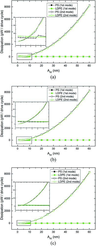Fig. 5 Energy dissipation curves of the second mode measured on PS-LPDE with varying free amplitudes A₀₂. Free amplitude (a) A₀₁ = 54 nm, (b) A₀₁ = 40 nm and (c) A₀₁ = 25 nm.

3.3. Virial

The virial theorem provides a way to relate phase to the time-averaged interaction force.^28,29 Virial can be interpreted as the average stored energy (potential energy) of the tip-sample interaction. When the net tip-sample force is attractive, the phase shift is greater than 90 degrees. As can be inferred from eqn (2), the virial is positive. On the contrary, when the tip scans in the net repulsive regime, the virial becomes negative. Fig. 6 shows the corresponding virial curves on the PS and LDPE portions for the two driving modes. Fig. 6(a)–(c) are plotted with different free amplitudes A₀₁ (54, 40 and 25 nm). In Fig. 6(a), the first mode virial curve of LDPE remains flat from 35 to 65 aJ, in which the amplitude and phase vary a little. The virial of PS becomes negative because of the repulsive tip-sample force at the phase reversal point A₀₂ = 8 nm. Similarly, the negative part of the virial curve remains from −17 to −69 aJ. The second mode virial of LDPE increases from 0.098 to 390 aJ when A₀₂ trends towards higher values from 1 to 60 nm. The virial of PS becomes negative at the phase reversal point and increases from −5.9 to 253 aJ when A₀₂ changes even more. As the free amplitude A₀₁ decreases, as shown in Fig. 6(b) and (c), the virial curves keep the same trend. However, it is clear that the difference in the two virial lines on PS and LDPE is smaller. Irrespective of the first mode or the second mode, the virial difference reflects the contrast of the image. The sum curves of virial for both modes on the PS and LDPE regions are also plotted in Fig. 6. The cross points of the PS and LDPE sum curves for different free amplitudes A₀₁ are consistent with the reversal points of the phase (Ø₁ and Ø₂).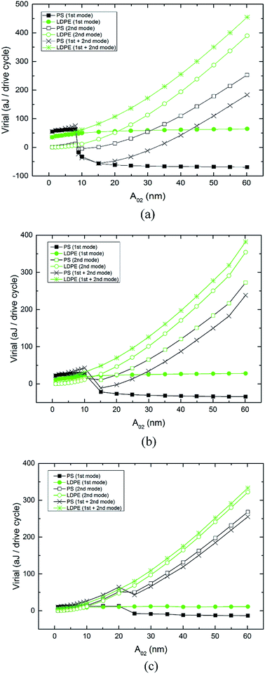

Fig. 6 Virial curves of the first mode, second mode and the sum of both modes measured on PS-LPDE with varying free amplitude A₀₂. Free amplitude (a) A₀₁ = 54 nm, (b) A₀₁ = 40 nm and (c) A₀₁ = 25 nm.

3.4. Contrast

To quantify image contrast at different free amplitudes and varying setpoint ratios, pixel values can be extracted and the histogram of response amplitude and phase from each AFM image can be calculated. The histogram of a continuous probability distribution with two modes can be obtained in one image for PS-LDPE. Then, the normalized histogram can be fitted using the following bimodal distribution function:³⁰where μ₁ and μ₂ are the means of the two normal distributions, and σ₁ and σ₂ are the standard deviations. For a mixture of two normal distributions, the mean and standard deviation are two main factors to define the average and quantify the amount of variation or dispersion of a set of phase values (0 < Ø < π). Ashman's D is employed to quantify the amplitude and phase image contrasts at different setpoint amplitude values. D > 2 is a necessary condition for a clean separation of two mixed normal distributions. Therefore, D is defined as the criterion to evaluate amplitude and phase contrasts. The equation can be written as follows:^30,31where μ₁, σ₁, μ₂ and σ₂ can be obtained by extracting the data and fitting the histograms. Fig. 7 shows the A₂, Ø₁ and Ø₂ contrast curves calculated by the Ashman's D equation. In Fig. 7(a), the contrast of A₂, Ø₁ and Ø₂ in regime I is about 10, and A₂, Ø₁ and Ø₂ show similar contrast. In regime II, the contrasts of Ø₁ and Ø₂ sharply increase, but the contrast of A₂ slightly drops. Moreover, the contrasts of A₂ in regime II are around or lower than the green short dash line D = 2, which is the discrimination line of contrast demarcation. Nevertheless, the contrast curves of A₂, Ø₁ and Ø₂ dramatically increase in regime III. Significantly, the Ø₂ contrast curve has the maximum value of 95.6, and the highest contrasts of A₂ and Ø₁ are 35.3 and 89.1, respectively. There is an evident advantage of Ø₁ and Ø₂ over A₂ in regime III, where greater A₀₂ are operated during bimodal experiments. Generally, the first mode free amplitude is more than an order of magnitude larger than the second mode free amplitude. If the second mode free amplitude is too large, there are some apparent response couplings resulting from the two exciting modes. Nevertheless, it is interesting that a greater A₀₂ might correspond to much better image contrast. As the free amplitude of first mode A₀₁ decreases, as shown in Fig. 7(b) and (c), the contrast curves present a similar law in regime III, but show lower best values. Moreover, the contrasts of Ø₂ also show significant advantages when the second free amplitudes A₀₂ are lower than 10 nm, as shown in Fig. 7(b) and (c).

Fig. 7 Phase contrast curves of different free amplitudes A₀₁. (a) A₀₁ = 54 nm, (b) A₀₁ = 40 nm and (c) A₀₁ = 25 nm. Regimes I, II and III are divided by the deep blue dot lines on the basis of phase reversals. The green short dash lines represent the reference value D = 2.

3.5. Setpoint ratio effects

To research the contrast of compositions, we also explored the dependencies of A₂, Ø₁ and Ø₂ associated with the amplitude setpoint ratio of A₀₁. Fig. 8 shows the contrast curves of A₂, Ø₁ and Ø₂ versus the setpoint ratio of A₀₁, where the free amplitude A₀₂ is set to 20 nm. When A₁/A₀₁ ≥ 0.65, where the tip mainly stays in the attractive regime, the curve of Ø₂ contrast stays higher than that of Ø₁ and A₂. When A₁/A₀₁ < 0.65, where the tip stays in the attractive regime in the LDPE region and repulsive regime in the PS region, the contrast of Ø₁ shows a significant advantage over Ø₂ and A₂. The maximum occurs near an A₁/A₀₁ ratio of about 0.35–0.5 for both Ø₁ and Ø₂. These results appear similar to the behavior observed in conventional monomodal AM-AFM for the dependence of the minimum distance with A₁/A₀₁. Therefore, there are multiple choices in terms of optimizing the contrast of compositions.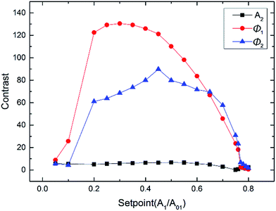

Fig. 8 A₂, Ø₁ and Ø₂ contrast curves dependence on the amplitude setpoint ratios of the first mode with A₀₂ = 20 nm.

4. Conclusions

We conducted bimodal experiments on a PS-LDPE polymer blend where different free amplitudes of the first flexural resonance mode and gradually increasing free amplitudes of the second mode are employed. Three regimes are divided based on the reversal of amplitude and phase curves, which also correspond to attractive and repulsive regimes. The energy dissipation power and virial for both modes are calculated to explain the enhanced phase contrast physically. Greater free amplitudes of the first mode and second mode present more dissipation and virial, and show significantly better compositional contrasts, particularly for the phase of the second mode. The results show that the phase contrast of the second mode increases about 9.5 times compared with that of the traditional results. Contrast is also closely related to the amplitude setpoint ratio of the first mode. Experiments illustrate that the second mode phase in high ratios (attractive regime) and the first mode phase in middle ratios (repulsive regime) show outstanding contrast. Regarding the complicated theories of these experimental phenomena, further research is needed. Understanding the energy changes and compositional contrast of bimodal AFM mode points is a way to distinguish and characterize soft polymeric materials and biological samples.

Acknowledgements

We thank Asylum Research engineers for helpful discussions. This research is financially supported by the National Natural Science Foundation of China (Grant Nos 51527901, 51375255 and 51321092).

References

1. R. Garcia and E. T. Herruzo, Nat. Nanotechnol., 2012, 7, 217–226.
2. S. Jesse, S. Kalinin, R. Proksch, A. Baddorf and B. Rodriguez, Nanotechnology, 2007, 18, 435503.
3. D. Platz, E. A. Tholen, D. Pesen and D. B. Haviland, Appl. Phys. Lett., 2008, 92, 153106.
4. B. J. Rodriguez, C. Callahan, S. V. Kalinin and R. Proksch, Nanotechnology, 2007, 18, 475504.
5. T. Rodriguez and R. Garcia, Appl. Phys. Lett., 2004, 84, 449–451.
6. J. R. Lozano and R. Garcia, Phys. Rev. Lett., 2008, 100, 076102.
7. A. Berquand, P. E. Mazeran and J. M. Laval, Surf. Sci., 2003, 523, 125–130.
8. S. Kawai, T. Glatzel, S. Koch, B. Such, A. Baratoff and E. Meyer, Phys. Rev. Lett., 2009, 103, 220801.
9. S. Santos, Appl. Phys. Lett., 2013, 103, 231603.
10. R. W. Stark, T. Drobek and W. M. Heckl, Appl. Phys. Lett., 1999, 74, 3296–3298.
11. E. T. Herruzo, A. P. Perrino and R. Garcia, Nat. Commun., 2014, 5, 3126.
12. N. F. Martinez, J. Lozano, E. T. Herruzo, F. Garcia, C. Richter, T. Sulzbach and R. Garcia, Nanotechnology, 2008, 19, 384011.
13. R. Proksch, Appl. Phys. Lett., 2006, 89, 113121.
14. A. M. Gigler, C. Dietz, M. Baumann, N. F. Martinez, R. Garcia and R. W. Stark, Beilstein J. Nanotechnol., 2012, 3, 456–463.
15. F. R. Service, Science, 2000, 289, 27–28.
16. D. Kiracofe, A. Raman and D. Yablon, Beilstein J. Nanotechnol., 2013, 4, 385–393.
17. T. E. Fisher, A. F. Oberhauser, M. Carrion-Vazquez, P. E. Marszalek and J. M. Fernandez, Trends Biochem. Sci., 1999, 24, 379–384.
18. I. Chakraborty and D. G. Yablon, Nanotechnology, 2013, 24, 475706.
19. S. Santos, Appl. Phys. Lett., 2014, 104, 143109.
20. R. W. Stark, Appl. Phys. Lett., 2009, 94, 063109.
21. S. An, S. D. Solares, S. Santos and D. Ebeling, Nanotechnology, 2014, 25, 475701.
22. E. T. Herruzo and R. Garcia, Appl. Phys. Lett., 2007, 91, 143113.
23. D. Kiracofe and A. Raman, Nanotechnology, 2011, 22, 485502.
24. G. Chawla and S. D. Solares, Appl. Phys. Lett., 2011, 99, 074103.
25. R. Garcia, J. Tamayo and A. S. Paulo, Surf. Interface Anal., 1999, 27, 312–316.
26. J. P. Cleveland, B. Anczykowski, A. E. Schmid and V. B. Elings, Appl. Phys. Lett., 1998, 72, 2613–2615.
27. J. Lozano and R. Garcia, Phys. Rev. B: Condens. Matter Mater. Phys., 2009, 79, 014110.
28. G. Stan, et al., Ultramicroscopy, 2009, 109, 929–936.
29. A. J. Diaz, B. Eslami, E. A. López-Guerra and S. D. Solares, J. Appl. Phys., 2014, 116, 104901.
30. D. Forchheimer, R. Forchheimer and D. B. Haviland, Nat. Commun., 2015, 6, 6270.
31. K. M. Ashman, C. M. Bird and S. E. Zepf, Astron. J., 1994, 108, 2348–2361.

---