
The low-temperature dynamic crossover in the dielectric relaxation of ice Ih
Ivan
Popov
 ab,
Ivan
Lunev
b,
Airat
Khamzin
b,
Anna
Greenbaum (Gutina)
c,
Yuri
Gusev
b and
Yuri
Feldman
*a
ab,
Ivan
Lunev
b,
Airat
Khamzin
b,
Anna
Greenbaum (Gutina)
c,
Yuri
Gusev
b and
Yuri
Feldman
*a
aThe Hebrew University of Jerusalem, Department of Applied Physics, Edmond J. Safra Campus, Givat Ram, Jerusalem, 9190401, Israel. E-mail: yurif@mail.huji.ac.il
bInstitute of Physics, Kazan Federal University, Kremlevskaya str.18, Kazan, 420008, Russia
cThe Hebrew University of Jerusalem, Racah Institute of Physics, Edmond J. Safra Campus, Givat Ram, Jerusalem, 9190401, Israel
First published on 10th October 2017
Abstract
Based on the idea of defect migration as the principal mechanism in the dielectric relaxation of ice Ih, the concept of low-temperature dynamic crossover was proposed. It is known that at high temperatures, the diffusion of Bjerrum and ionic defects is high and their movement may be considered to be independent. Simple switching between these two mechanisms leads to a dynamic crossover at ∼235 K. By introducing coupling between the Bjerrum and ionic defects, it is possible to describe the smooth bend in the relaxation time at low temperatures in ice Ih. However, because the mobility of Bjerrum orientation defects slows down at low temperatures, they may create blockages for proton hopping. The trapping of ionic defects by L-D defects for a long period of time leads to an increase in the relaxation time and causes a low-temperature crossover. This model was validated by experimental dielectric measurements using various temperature protocols.
Introduction
Despite its apparent simplicity, ice Ih presents a quite complex dielectric relaxation behavior. These complexities in the investigation of ice are related to the absence of repeatability in experimental dielectric data provided by various research groups. Thus, whereas the dielectric relaxation times in previous studies1,2 follow the Arrhenius law down to 200 K, the results of other studies3–11 reveal crossover in the vicinity of temperature Tc ≈ 235 K (see Fig. 1). Furthermore, detailed studies of ice over a wide range of temperatures and frequencies4–7,9 have shown deviations between the dielectric results in the low-temperature range (Fig. 1). As proposed in ref. 12, such variable results are probably the result of the method of ice preparation and the temperature protocol of the dielectric study. This idea was verified by Sasaki et al.,9 who performed the important experiment of examining ice samples prepared by different methods. It was shown that an ice sample prepared with stirring (to avoid rapid ice crystallization) does not exhibit a high-temperature crossover, whereas the relaxation time of the samples produced without special treatment demonstrates a behavior similar to that in previous studies,4,6,7 but with appreciable deviations at very low temperatures (Fig. 1). | ||
| Fig. 1 The temperature dependences of the relaxation time of ice Ih. Here, only the widest temperature studies are displayed. The gray squares and circles are attributed to the single crystal data taken from ref. 6 and 7; the gray triangles correspond to polycrystals and are taken from ref. 4. The data defined by the black circles, squares and diamonds are taken from ref. 9. The large filled rectangles denote the range where the high-temperature dynamic crossover is observed. The black curved arrow denotes the low-temperature crossover. | ||
In addition to experimental problems, the theoretical investigation of the dielectric relaxation in ice is lagging. In fact, Jaccard's model13,14 has been the main detailed quantitative treatment in the literature15–17 regarding the dynamic electrical properties of ice. In this model, both ionic H3O+/OH−![[thin space (1/6-em)]](https://www.rsc.org/images/entities/char_2009.gif) 18 and orientation Bjerrum defects19–21 were considered as the mechanisms of electrical conductivity and dielectric polarization in ice. Recently, we considerably expanded this idea12 and explained both the dynamic crossover at Tc ≈ 235 K and the variation of dielectric spectral broadening at this temperature. However, the theory we developed in its current state cannot be applied to describe the low-temperature crossover where the activation energy begins to increase again (Fig. 1). As of now, no reliable theory exists that may suggest a good interpretation of this phenomenon, apart from some qualitative explanations. For example, Johari et al. in ref. 5 suggested that this crossover may be related to a transition back to the mechanism that is responsible for the high-temperature range. At the same time, the answer to this question is extremely important, as it may help us understand the closely related behavior of hydration water in various powders, including hydrated proteins. Actually, the available experimental data of hydrated powders at low temperatures show11,22–24 that the relaxation time of the hydrated water in some systems is either a continuation part of the relaxation time of bulk ice at low temperatures or is parallel to it. Thus, discovering the mechanism of the low temperature crossover in ice allows us to elucidate the enigmas of hydration water dynamics.
18 and orientation Bjerrum defects19–21 were considered as the mechanisms of electrical conductivity and dielectric polarization in ice. Recently, we considerably expanded this idea12 and explained both the dynamic crossover at Tc ≈ 235 K and the variation of dielectric spectral broadening at this temperature. However, the theory we developed in its current state cannot be applied to describe the low-temperature crossover where the activation energy begins to increase again (Fig. 1). As of now, no reliable theory exists that may suggest a good interpretation of this phenomenon, apart from some qualitative explanations. For example, Johari et al. in ref. 5 suggested that this crossover may be related to a transition back to the mechanism that is responsible for the high-temperature range. At the same time, the answer to this question is extremely important, as it may help us understand the closely related behavior of hydration water in various powders, including hydrated proteins. Actually, the available experimental data of hydrated powders at low temperatures show11,22–24 that the relaxation time of the hydrated water in some systems is either a continuation part of the relaxation time of bulk ice at low temperatures or is parallel to it. Thus, discovering the mechanism of the low temperature crossover in ice allows us to elucidate the enigmas of hydration water dynamics.
In this work, we shall present the development of the theory proposed in our recent study.12 We shall try to explain the temperature dependence of the relaxation time and the broadening parameter over a whole temperature range as presented in Fig. 1, including the low-temperature crossover. To validate the proposed model, we have performed dielectric measurements using various specific temperature protocols.
Basic principles of the dielectric relaxation in ice
The “wait-and-switch” model16,17,25–27 is commonly accepted as the most suitable model for the description of the dielectric relaxation in ice. According to this model, the reorientations of a water dipole are assumed to be the switching between different dipole directions (in accordance with the Bernal–Fowler–Pauling rules28,29) rather than its continuous diffusion. Furthermore, these reorientations occur only when the water molecule encounters an appropriate defect in the H-bond network, otherwise the water molecule remains in a waiting mode.27 In this case, the term “defect” refers to either orientation L-D Bjerrum defects19–21 or ionic H3O+/OH− defects.18,30 The advantage of this approach is that it simplifies the theoretical picture: instead of a many-body interaction problem, one can consider a random walker problem of defect motion. Based on this idea, we succeed in deriving the relationship between the complex dielectric permittivity ε*(ω) and the mean square displacement (MSD) of the defects 〈r2(t)〉12 | (1) |
 is the partial conductivity that may be related to defect migration, and
 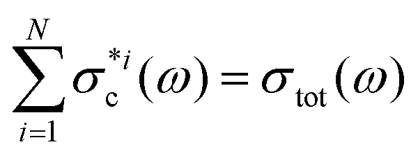 is the total conductivity defined by the contributions of all the types of defects. In the same work,12 using the relationship (1), we explained the high-temperature crossover at Tc ≈ 235 K, considering only two terms in eqn (1), which correspond to the combined effect of the ionic and orientation defects. As a result, we derived an expression that describes both the bend in the relaxation time and the broadening of the loss peak at this temperature. This is in agreement with the idea31 and experimental observations32,33 that the origin of the high-temperature crossover is a shift in the relaxation mechanism via orientation L-D defects to that of relaxation via ionic H3O+/OH− defects. It was concluded12 that although the activation energy of L-D defect migration is higher than that of ionic defect migration, their overall number exceeds the total amount of ionic defects. This means that at high temperatures when it is easier to overcome the potential barrier, the probability of the total polarization being changed by L-D defects is higher due to their larger quantity. However, with decreasing temperature, it becomes more difficult to overcome the higher activation barrier and the probability of dipole polarization due to the ionic defects increases.
Nevertheless, this theoretical result cannot be directly extended to the much lower temperature range to describe the second bend in the relaxation time.12 To explain this puzzling crossover, we are compelled to take into account additional physical phenomena, which become significant at low temperatures.
The blockage of the ionic defects by the orientation defects
In a previous work12 that considered the combined migration of ionic and orientation defects, we assumed that the defects diffuse independently and are not correlated with each other (Fig. 2a). However, the Bjerrum orientation defects may block proton hopping from one water molecule to another (Fig. 2b), i.e. they may prevent the diffusion of ionic defects. Moreover, moving protons “block their own paths”, i.e. a proton's movement creates orientations of water molecules along its trace, such that a subsequent proton cannot pass that way. To unblock proton hopping, the involvement of water molecule rotation as a whole is necessary.17,32 For example, one of the water molecules (marked in blue in Fig. 2b) may turn in such a way that the oxygen atom will be oriented towards the proton (curved blue arrows in Fig. 2b), providing the possibility for further proton hopping. In other words, the L-defect in Fig. 2b may move and unblock the way for the proton. An alternative option is that the whole H3O+ complex may rotate and move the blocked proton onto a free unobstructed path, as shown in Fig. 2c.34 We can also consider the rotation of the H3O+ complex as a type of orientation defect. Thus, proton migration must be considered to be restrictive due to the activity of the orientation defects.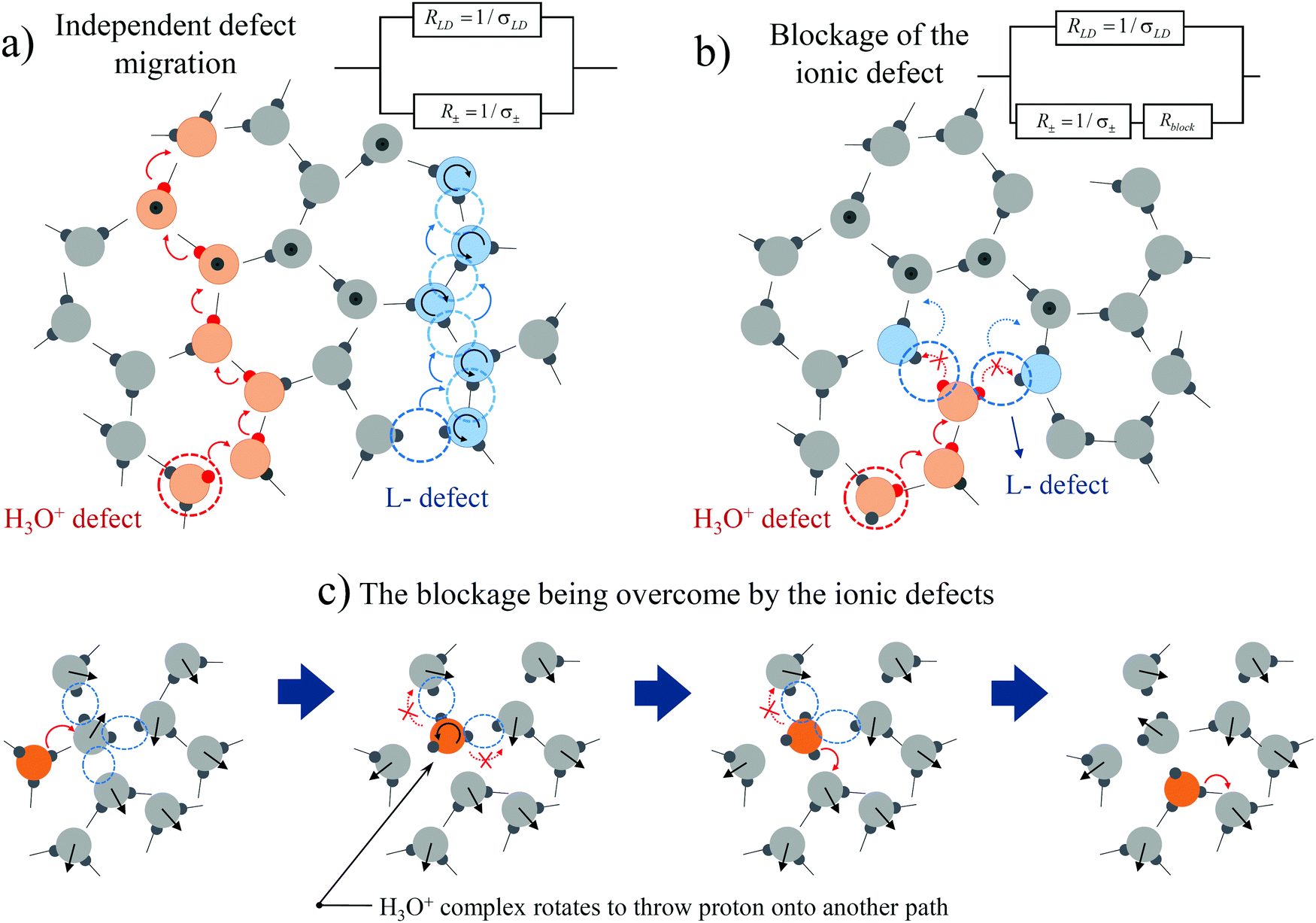 | ||
| Fig. 2 The schematic presentation of the defect migrations. (a) Independent diffusion of ionic and orientation defects. In this case, we have two parallel relaxation channels. (b) Here, we demonstrate one of the possible types of interaction between defects: the blockage of ionic defect H3O+ by the orientation L-defect. (c) The overcoming of the blockage by the ionic defect via rotation of the H3O+ complex and the throwing of the blocked proton onto another bond. In this case, the relaxation channel driven by the ionic defects consists of two resistances: R±(ω) and Rblock(ω). | ||
At high temperatures, when the defect diffusion is fast enough and the retention time of ionic defects in traps is not that large, we may consider this migration to be uncorrelated. In this case, we may speak about two parallel relaxation mechanisms via orientation and ionic defects. We can then describe the system by an equivalent circuit with two resistances (see the scheme in Fig. 2a): resistance of the orientation L-D defects RLD(ω) = 1/σLD(ω) and the ionic defects R±(ω) = 1/σ±(ω) (hereinafter the subscript “±” is attributed to the ionic defects). Using eqn (1) and the rule for parallel connections, we have
 | (2) |
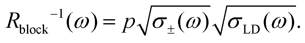
This expression was comprehensively examined in ref. 12, where the high-temperature crossover was described. However, at low temperatures, the effect of blockage of the ionic defects becomes more significant due to slowing down of the orientation L-D defects. The blocked anionic or cationic defects may be held in traps over a long time period until the orientation defects unblock the way for the next proton hop. Thus, instead of the usual proton hopping (obeying the Grotthuss mechanism18), we should consider the diffusion of coupled orientation–ionic aggregates.31 In this case, we should add the additional subsequent resistance Rblock(ω) in the equivalent scheme for the proton relaxation channel (see the scheme in Fig. 2b). Calculating the total conductivity of this scheme, we obtain
 | (3) |
According to the relationship (1), the conductivity is proportional to the MSD. So for the L-D and ionic defects, we have σLD(ω) = RLD−1(ω) ∼ 〈rLD2(ω)〉 and σ±(ω) = R±−1(ω) ∼ 〈r±2(ω)〉. As mentioned above, the Rblock(ω) may be associated with the correlated migration of the orientation and ionic defects, and in the first approximation, we may assume that Rblock−1(ω) ∼ 〈r±(ω)rLD(ω)〉. In turn, in the case of a strong correlation, we may write that  .35 Thus the Rblock−1(ω) may be defined as follows:
 | (4) |
Here, the parameter p characterizes the degree of correlation and may depend on the concentration of trapped protons, the trap period, etc. Substituting eqn (4) into (3) and using eqn (1), we can rewrite eqn (3) as follows:
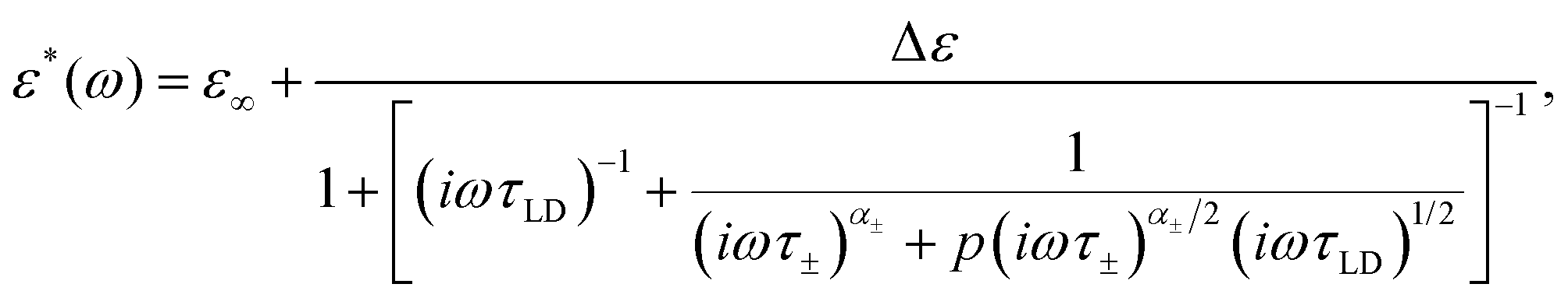 | (5) |
 | (6) |
Here, we have assumed that orientation defects obey the normal diffusion behavior, whereas the ionic defects are characterized by anomalous diffusion
 | (7) |
This assumption is necessary in order to describe the broadening of the ice loss peak below the high-temperature crossover.12 It was seen4,6,12 that above Tc ≈ 235 K the complex dielectric permittivity is fitted well by the Debye law, but below Tc, the dielectric spectra start to obey the Cole–Cole law. The reasons for the anomalous proton movement can be very diverse. There are many models that have proposed this anomalous behavior.36–38 For example, as we mentioned in ref. 12, the same trapping of protons by the orientation defects may lead to their deviation from the normal diffusion law. In this paper, we shall not study this problem in depth. We simply accept this experimental observation and focus on the question of the low-temperature crossover. In the case where the degree of correlation p is small or the L-D conductivity is large (the case at high temperatures), we obtain the previous expression (2).
Eqn (5) presents a nonlinear expression. However, if the α± parameter value is close to one, we can approximate this relationship by the Cole–Cole function (see the Appendix)
 | (8) |
 | (9) |
 | (10) |
Fig. 3 shows the model data of τ and α at different values of p. It is clear that eqn (9) presents the relaxation time behavior similar to the experimental data shown in Fig. 1.
 | ||
| Fig. 3 The model data of the τ and α at different values of degree of correlation p. Here we designate (as an example) α± = 0.9. Red dashed lines, corresponding to τLD and τ±, obey the simple Arrhenius law with energy of activation ELD = 55 kJ mol−1 and E± = 16 kJ mol−1 and pre-exponential factors 6 × 10⁻¹⁶ s and 3 × 10⁻⁷ s. | ||
In the limit cases, we have either a single high-temperature crossover (p = 0) or else the crossovers are completely missing (p ≫ 1). The broadening parameter α decreases down to α± in the middle temperature range, but during the low-temperature crossover it increases to the average value of the power parameters of L-D and ionic defects (1 + α±)/2. The larger value of the parameter p corresponds to the stronger blockage of the proton movement. At the limit p → ∞, all protons are trapped and dielectric relaxation is driven by the L-D defects and the orientation–ionic aggregates.31 Such a behavior was observed e.g. in Auty and Cole's study1 and in recent measurements of ice samples prepared by stirring9 (as shown in Fig. 1). The behavior similar to the case of p = 0 is probably observed in the single H2O crystal6 (see Fig. 1); however, for the single D2O crystal the low-temperature crossover was detected.7
In the next section we shall verify our theoretical results experimentally for α(T) and τ(T). Moreover, we shall try to understand on what parameter p is dependent. Towards this aim, we performed specific dielectric measurements using different temperature protocols.
Materials and methods
All dielectric measurements were performed in the frequency range of 0.01 Hz–1 MHz using a BDS Concept-80 dielectric spectrometer (Novocontrol, Germany) with automatic temperature control by a Quatro Cryosystem with a precision of 0.5 °C. The sample cell for the dielectric experiments consists of a parallel plate capacitor containing electrodes with actual diameters of 16.2 mm spaced by a Teflon ring of diameter 7.1 mm. The accuracy of the dielectric measurements was ±3% for the real and imaginary parts of the complex dielectric permittivity. The measurements were performed independently in two different laboratories. The equipment of the Dielectric Spectroscopy Laboratory of Applied Physics, the Hebrew University of Jerusalem (Israel), and the Federal Center of Shared Equipment FCKP FChI of Kazan Federal University (Russia) were used.The following temperature protocols were utilized:
(1) Cooling temperature protocol: the cell filled with bi-distilled H2O water was cooled from room temperature down to 263 K at a rate of 1 K min−1. The system was maintained at this temperature for 1.5 hours. The sample was then measured over the temperature interval of 263 K down to 139 K with a step of 3 K. This temperature protocol was performed three times.
(2) Hysteresis temperature protocol: the cell filled with bi-distilled H2O water was cooled from room temperature down to 263 K at a rate of 1 K min−1. The system was maintained at this temperature for 1.5 hours. The sample was measured over the temperature cooling interval from 263 K down to 139 K with a step of 3 K, and then on heating from 139 K up to 263 K with a step of 3 K, and then again upon cooling from 263 K down to 155 K with a step of 3 K.
(3) Annealing temperature protocol: the cell filled with bi-distilled H2O water was cooled from room temperature down to 263 K at a rate of 1 K min−1. The system was maintained at this temperature for 1.5 hours. The sample was then measured over the temperature interval of 263 K to 206 K with a step of 3 K. At this temperature, cooling was stopped. At 206 K the sample was annealed and measured every 10 min for 65 hours.
(4) Quench temperature protocol: the cell filled with bi-distilled H2O water was quenched from room temperature down to 139 K at a rate of 12 K min−1. The system was maintained at this temperature for 1 hour. The sample was then measured at temperature intervals while heating from 139 K up to 263 K with a step of 3 K, and then while cooling from 263 K down to 139 K with a step of 3 K.
Results and discussion
The typical dielectric spectra are presented in Fig. 4. A clear relaxation peak and an electrode polarization (EP) effect at low frequency is observed. It is worth noting that usually the EP in data treatment either is not taken into account at all or is described by Jonscher's correction.39 However, Jonscher's term ∼(iω)−n presents a simple power law behavior and in many cases does not conform to the experimental data. Indeed, very often, kinks/bends40–43 on the tail of the EP are detected, which cannot be described by Jonscher's correction. There are many theoretical models which improve the description of the EP,44,45 however here we shall use the results of our previous studies,46,47 where this issue was considered in detail. In these studies, it was shown that the tail of the EP should be described by the following frequency-dependent term | (11) |
 | (12) |
 | ||
| Fig. 4 The typical dielectric spectra for ice. Circles present the dielectric data measured in the first experiment of the cooling temperature protocol (see Material and methods). The black line represents the total fitting curve according to eqn (12); the corresponding contributions of the individual terms are represented by the colored lines: conductivity (magenta), EP (blue), and relaxation (red) terms. | ||
The fitting of the typical dielectric spectra of ice viaeqn (12) and the contributions of the individual terms are presented in Fig. 4. The correct description of the EP tail improves the accuracy of the fitting of the relaxation term. By itself, the EP term is interesting for supplementary studies, but in our measurements due to experimental limitations, we are only able to obtain its fitting parameters in a narrow temperature interval (below T < 220 K the EP tail moves beyond the frequency window). In the current study, we focus on the dynamic crossover of the main relaxation peak, and omit the analysis of the EP term.
Another issue that appears in the dielectric data treatment of ice is the appearance of the additional process at very low temperatures. In Fig. 5, the normalized dielectric losses of ice are presented at several temperatures. Note that the spectrum at low temperatures (e.g. at 139 K in Fig. 5) cannot be fitted well by the Cole–Cole eqn (8) and the additional process should be introduced at low frequencies. This process appears in all our measurements and its origin is not clearly established at the present time. It is most likely caused by the cracks that appear in the ice during cooling,49–51 or else it could be related to the inhomogeneity of ice freezing near the electrode. In addition, it may be attributed to a new intrinsic property of the ice dynamics at low temperatures. In the current study, we are interested in the behavior of the main relaxation peak, but the presence of this unexplored process prevents the extraction of the correct temperature dependences of the fitting parameters (Δε, α, and τ of the relaxation terms in eqn (12)). Therefore, we have performed the data fitting viaeqn (12) down to 152 K only.
 | ||
| Fig. 5 Normalized data (Master plot) of the dielectric loss of ice at different temperatures in the first experiment of the cooling temperature protocol (see Material and methods). Each spectrum is normalized by the amplitude of the main dielectric peak, and each frequency scale by the characteristic of the same peak. The model data of the Cole–Cole law are represented by the solid line. The additional relaxation process at low temperatures is depicted by the arrow. | ||
(1) Cooling temperature protocol
In this temperature protocol, the ice sample was measured during slow cooling. The temperature dependences of the fitting parameters of the relaxation terms (Δε(T), α(T), and τ(T)) are presented in Fig. 6a and b. The appearance of the additional process at low temperatures leads to an increase in the fitting error in the broadening parameter and the dielectric strength, while the relaxation time is a more robust parameter. The error bars are shown for the first experiment, and this distribution of the error bars for the other experiments is similar. In Fig. 6, we also present the previous results of Kawada6,7 and Johari4,5 studies. It is worth noting about the debates regarding the existence of anisotropy in a single ice Ih crystal. The Kawada's previous experimental and theoretical studies6,52 revealed the anisotropic properties of dielectric constants in ice. The measured temperature dependences of Δε‖(T) and Δε⊥(T) are presented in Fig. 6a (we kept the notations). However, Johari's study of a single ice crystal discovered no difference between the Δε‖(T) and Δε⊥(T).2 Furthermore, Johari's next study5 provided similar values and temperature dependences of dielectric strength for polycrystalline and single ice crystals (in Fig. 6a the results for polycrystals are shown). The various computer simulation studies also cannot resolve this issue at present.53–56 Our results for Δε(T) are within this interval ([Δε‖, Δε⊥]) provided by Kawada6 and exhibit a correct temperature behavior (see Fig. 6a), which should obey the Curie–Weiss law (Δε(T) ∼ 1/T), as well as in previous ice studies.4–6 | ||
| Fig. 6 The temperature dependences of the (a) dielectric strength and (b) broadening parameter (upper panel) and relaxation time (lower panel) in the cooling temperature protocol. The three measurements are shown by the open symbols. For the first experiment (diamond symbols), the error bars are shown; for the relaxation time the error bars lie within the symbol size. For the other experiments, the error bars are similar. Also, the previous data of Kawada,6,7 and Johari4,5 are represented by full symbols. The data in Fig. 6a present the linear dependence in the plane 1000/Δε vs. T that corresponds to the Curie–Weiss law. The parameters Δε‖(T) and Δε⊥(T) define the dielectric strength of the single crystal oriented parallel, and perpendicular to an electric field, respectively taken from ref. 6. The blue line in Fig. 6b corresponds to the model curve of eqn (9). | ||
The most interesting result is that of the temperature dependences of α(T) and τ(T). They both present the similar behavior expected according to our model at the correlation parameter p ≪ 1 (see Fig. 3). The parameter α(T) has a minimum in the vicinity of the high-temperature crossover (min(α(T)) ≈ α±) and reaches the saturation value (α(T → 0) ≈ (α± + 1)/2) below the low-temperature crossover. The blue line represents the fitting curve provided by the model eqn (9), where τLD(T) and τ±(T) obey the Arrhenius law with activation energies ELD = 59 kJ mol−1 and E± = 16 kJ mol−1 and pre-exponential factors 2 × 10⁻¹⁶ s and 2 × 10⁻⁷ s, respectively. The proton diffusion parameter was obtained as α± ≈ 0.91 and the correlation coefficient was set as p = 0.003. Although the model curve does not fit α(T) well, our model, despite its simplicity, predicts the main tendency in the temperature behavior of the relaxation time and the broadening parameter in ice. Obviously, these correlation and diffusion parameters, p and α±, are also functions of temperature. Taking this into account, we would succeed in obtaining a much better fitting curve, yet even when we assumed that they are constants, we obtain good agreement with experimental results.
As mentioned in the introduction, the repeatability of the dielectric results is problematic, especially at low temperatures. Most likely this is because the microstructure (polycrystallinity) of ice depends on the temperature protocol, leading to a variability in the correlation parameter p. Indeed, a series of studies49–51 using X-ray diffraction topography revealed stacking faults in ice crystals. The faults present self-interstitial defects whose concentration rapidly increases during cooling. However, any micro dislocations and cracks in the ice, on the one hand, may serve as the source of the orientation L-D defects, and on the other hand, may be considered as additional suppressors for long-range proton migration. Therefore, it makes sense to verify how the different temperature protocols influence the dielectric results.
(2) Hysteresis temperature protocol
In this protocol, we intended to observe to what extent the structure of the ice sample and its dynamics are stable over a broad temperature range. The ice was cooled down to 139 K, heated up to 263 K, and cooled back down again. The dielectric results after data treatment are shown in Fig. 7a and b. As can be seen, the results are slightly different from the previous cooling protocol, but the hysteresis is almost negligible. There is only a weak discrepancy of the results at low temperatures that is probably caused by the deformation of the microstructure of the ice sample.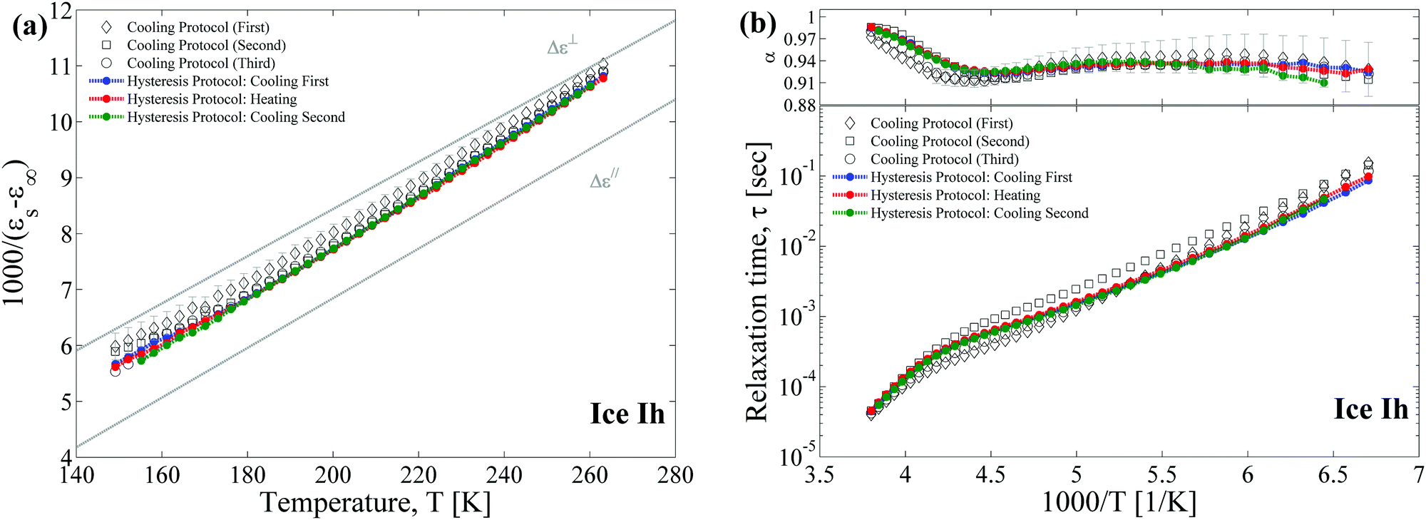 | ||
| Fig. 7 The temperature dependences of the (a) dielectric strength and (b) broadening parameter (upper panel) and relaxation time (lower panel) in the hysteresis temperature protocol. The open gray symbols correspond to the previous measurements of the cooling temperature protocol. The blue line is attributed to the ice cooling down to 139 K, the red line represents the heating up to 263 K, and the green line represents the cooling back down to 155 K. | ||
(3) Annealing temperature protocol
According to the results of the X-ray topography studies,49–51 cracks should appear in the ice during the annealing procedure. Annealing of the ice sample was performed at 206 K for 65 hours. Assuming that cracks may serve as a source of the orientation defects, we expected to observe an increase in the relaxation time during annealing below the high-temperature crossover (206 K was chosen for this reason) due to the growth of the correlation between the L-D and ionic defects. The results are presented in Fig. 8a–c. Fig. 8a demonstrates the difference in the dielectric strength, Δε(T), from the previous cooling temperature protocol, although the sample preparation was the same. Δε(T) shows lower values, but it is still in the range ([Δε‖, Δε⊥]) and obeys the Curie–Weiss law. The broadening parameter, α(T), also differs from those measured previously, namely the minimum is shifted to the low-temperature range. Thus, the way the ice freezes may vary even under the same sample preparation conditions, leading to a significant deviation in the dielectric response. However, no changes in relaxation behavior were detected during annealing. The deviation of the dielectric data is negligible over the entire frequency range (see Fig. 8c). Most probably unlike other studies,49–51 in our ice sample either the cracks were too big, or else they formed in insufficient quantity (the temperatures below the high temperature crossover are too low for crack formation) to impact dielectric relaxation at a microscopic level. | ||
| Fig. 8 The temperature dependences of the (a) dielectric strength and (b) broadening parameter (upper panel) and relaxation time (lower panel) in the annealing temperature protocol. The open gray symbols correspond to the previous measurements in the cooling temperature protocol. The temperature at which annealing started is depicted by the blue arrow. In (c) the dielectric spectra of the ice at different annealing times are shown. In addition, the total fitting curve according to eqn (12) is presented (black line). The corresponding contributions of the individual terms are presented by the dashed color lines: conductivity (magenta), EP (blue), and relaxation (red) terms. | ||
(4) Quench temperature protocol
In this protocol, we attempted to obtain non-equilibrium states in the sample, since fast cooling should lead to large disturbances in ice crystallization. The α parameter is the most sensitive one to the presence of tensions (probably due to microcracks formation) within the ice. Fig. 9b shows clearly that α decreases at low temperatures, and its behavior does not fit our model. However, after heating and re-cooling, the ice achieves an equilibrium state and its characteristics are similar to those of the sample in the cooling temperature protocol. The dielectric strength Δε(T) again shows the lower values as in the annealing temperature protocol.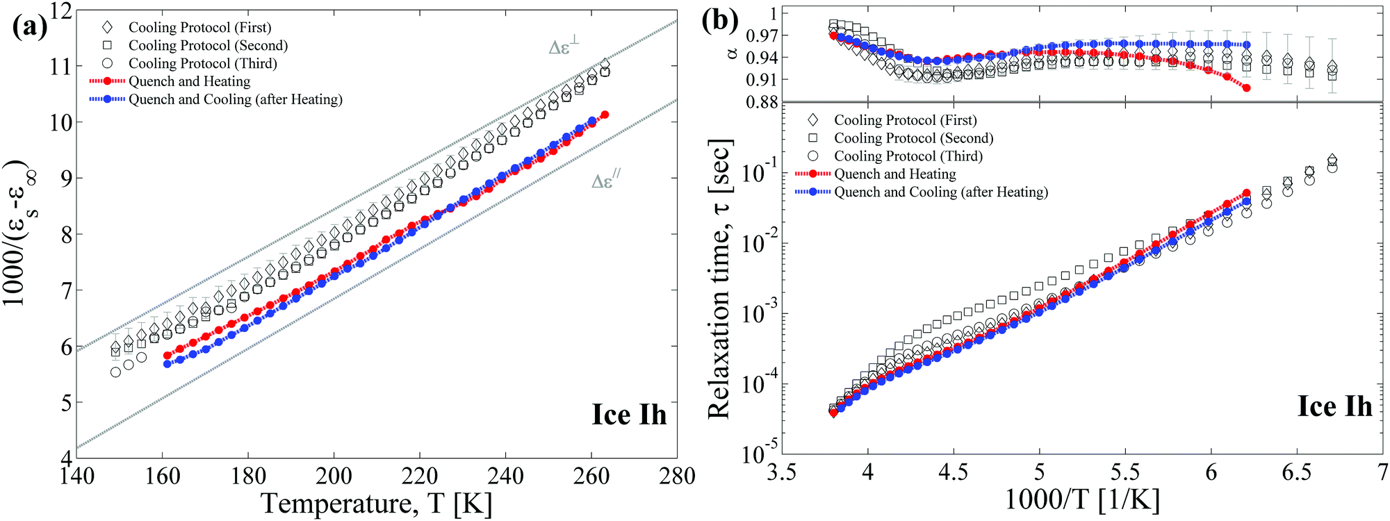 | ||
| Fig. 9 The temperature dependences of the (a) dielectric strength and (b) broadening parameter (upper panel) and relaxation time (lower panel) in the quench temperature protocol. The open gray symbols correspond to the previous measurements of the cooling temperature protocol. The red line is attributed to the heating up of the ice sample after quenching; the blue line represents the re-cooling. | ||
The experimental results we obtained prove the aforementioned assumption that the dielectric response of the ice Ih strongly depends on its preparation and the applied temperature protocol. Furthermore, even if the same procedure is performed for ice preparation, we obtain a variation in the dielectric response. We suggest that this phenomenon is related to an unrepeatability of the microstructure of the polycrystalline sample. In terms of our model, we may claim that different microstructures of ice affect the migration of the L-D and ionic defects, and in particular they influence the coupling between them. The latter property defines the dynamics at low temperatures, where we observe the largest discrepancy in the experimental results. At high temperatures, the mobility of the defects is high, averaging any deviations in ice preparation. Therefore, all measurements provide approximately the same values of the dynamic parameters (α, τ) above the high temperature crossover (T > 235 K). In view of these facts, we may propose an explanation of the result obtained in ref. 9, where the absence of the high temperature crossover was detected in the ice sample prepared by the stirring procedure (see Fig. 1). Most likely, the stirring procedure causes tensions to develop within the ice lattice that, in turn, lead to micro-crack formation during cooling. A large number of cracks (in the case of high tension) can prevent proton migration and switch off the relaxation mechanism driven by the only ionic defects. In our model, this corresponds to the strong correlation between the L-D and ionic defects, p ≫ 1 (see Fig. 3), when the orientation–ionic aggregates appear.31
Furthermore, the variation of the results for the dielectric constant presented in Fig. 6a, 7a, 8a and 9a suggests that the difference in Kawada's data6 for Δε‖(T) and Δε⊥(T) is also the result of unrepeatability of sample preparation even for a single ice crystal. The micro-crack formation in the ice crystal may lead to different values of the dielectric constant. Thus, the ice may not have anisotropy as it was shown by Johari.2 Thereby, this problem requires an additional comprehensive investigation.
Conclusion
In this work, we developed the “wait-and-switch” model based on the idea of defect migration as the principal mechanism of the dielectric relaxation in ice. In our previous studies, this model was effectively applied to explain the dielectric response in bulk water57 and the high-temperature crossover12 in bulk ice. In the current research using this model, we have succeeded in elucidating the origin of the low-temperature crossover in ice, and can present the reasons why this crossover was not observed in some studies. Thus, within the context of the same idea, we can describe the dielectric relaxation in water in its different phases over a wide range of frequencies and temperatures.Briefly, the framework of dielectric relaxation may be presented as follows. In general, two types of defects coexist in water: orientation and ionic (proton hopping) defects. In the liquid state,57 the migration of the orientation defects is the dominant mechanism due to their huge number in comparison to the ionic ones (the abundance of the orientation defects actually defines the liquid's properties). Proton hopping also takes place, but its effect seems to be negligible with regard to dielectric polarization. The normal diffusion of the orientation defects defines the Debye type of dielectric relaxation. At the phase transition from liquid to bulk ice, the amount of orientation defects decreases drastically and their activation energy increases (up to ∼54 kJ mol−1), as a result of the ordering of the H-bond network in the crystalline ice structure.12 As a consequence, the relaxation of ice slows down drastically, and the loss peak jumps from the GHz to kHz region. Nevertheless, at high temperatures in ice, the overall number of the orientation defects still exceeds that of the ionic ones, and they continue to play the leading role in dielectric relaxation. Furthermore, their normal diffusion behavior still generates Debye-type relaxation. However, as temperature decreases, it becomes more and more difficult to overcome the higher barrier for the orientation defects, and so the dielectric relaxation mechanism shifts to that of the ionic defects (where the activation energy is lower by a third). Moreover, the anomalous diffusion of the protons leads to the Cole–Cole relaxation law. This is a reason for the high-temperature crossover.
In the current study, we took into account the fact that the orientation and ionic defects are not equivalent. Unlike the latter, the orientation defects may block proton hopping from one water molecule to another. Thus, the proton movement is not free and they may be trapped by the L-D defects. At high temperatures, this effect is not as pronounced because the retention time in the traps is relatively short due to the fast defect diffusion rate. However, as the temperature decreases, the ionic defects may be trapped for longer time periods due to the slowing down of the L-D defect diffusion rate. This leads to an increase in the relaxation time and originates the low-temperature crossover. At low temperatures, strong coupling exists between the orientation and ionic defects, and it is more appropriate to discuss the idea of the orientation–ionic aggregates rather than to discuss each type of defect separately. In this case, the dynamical parameters of the aggregates (α, τ) are the average of those of the orientation and ionic defects (see Fig. 3, e.g. where the total broadening parameter tends toward (α± + 1)/2).
Finally, we note that the model presented here and in previous papers12,57 is applicable, not only to bulk ice and water but also to the hydration water in various systems (e.g. in proteins23), where the concept of defects can be introduced. Furthermore, we emphasize that the approach we have presented of defect migration allows for the reduction of the many-body interaction problem of H-bonded systems to the well-examined problem of random walk.
Conflicts of interest
There are no conflicts to declare.Appendix
To reduce eqn (8) to the Cole–Cole law, we may use the outcomes of Appendix B from previous work.12 It was shown that in the case of Δα = |α1 − α2|/2 ≪ 1, we may write| (iωτ1)α1 + (iωτ2)α2 = (iω〈τ〉)〈α〉 | (A.1) |
 | (A.2) |
Applying these relationships twice to eqn (8) and substituting parameters α1 = α±, α2 = (α± + 1)/2 and the corresponding relaxation times, we have
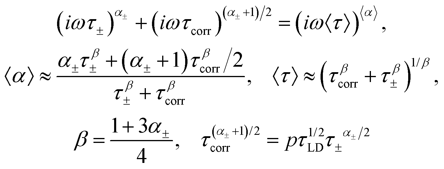 | (A.3) |
 | (A.4) |
Acknowledgements
This work was partly supported by the Russian Government Program of Competitive Growth of Kazan Federal University. A. Kh. acknowledges the support from the subsidy allocated to Kazan Federal University for performing the state assignment in the area of scientific activities (# 3.2166.2017/4.6). I. L. acknowledges the support from the subsidy allocated to Kazan Federal University for the state assignment in the sphere of scientific activities (3.7597.2017/7.8).References
- R. P. Auty and R. H. Cole, J. Chem. Phys., 1952, 20, 1309–1314 CrossRef CAS.
- G. P. Johari and S. J. Jones, J. Glaciol., 1978, 21, 259–276 CrossRef CAS.
- S. R. Gough and D. W. Davidson, J. Chem. Phys., 1970, 52, 5442–5449 CrossRef CAS.
- G. P. Johari and S. J. Jones, Proc. R. Soc. London, Ser. A, 1976, 349, 467–495 CrossRef CAS.
- G. P. Johari and E. Whalley, J. Chem. Phys., 1981, 75, 1333–1340 CrossRef CAS.
- S. Kawada, J. Phys. Soc. Jpn., 1978, 44, 1881–1886 CrossRef CAS.
- S. Kawada, J. Phys. Soc. Jpn., 1979, 47, 1850–1856 CrossRef CAS.
- S. S. N. Murthy, Phase Transitions, 2002, 75, 487–506 CrossRef CAS.
- K. Sasaki, R. Kita, N. Shinyashiki and S. Yagihara, J. Phys. Chem. B, 2016, 120, 3950–3953 CrossRef CAS PubMed.
- O. Worz and R. H. Cole, J. Chem. Phys., 1969, 51, 1546–1551 CrossRef.
- N. Shinyashiki, W. Yamamoto, A. Yokoyama, T. Yoshinari, S. Yagihara, R. Kita, K. L. Ngai and S. Capaccioli, J. Phys. Chem. B, 2009, 113, 14448–14456 CrossRef CAS PubMed.
- I. Popov, A. Puzenko, A. Khamzin and Y. Feldman, Phys. Chem. Chem. Phys., 2015, 17, 1489–1497 RSC.
- C. Jaccard, PhD thesis, Institut de Physique, EPF, 1959 DOI:10.3929/ethz-a-000099624.
- C. Jaccard, Phys. Kondens. Mater., 1964, 3, 99–118 CrossRef CAS.
- D. S. Eisenberg and W. Kauzmann, The structure and properties of water, Clarendon Press, Oxford University Press, Oxford, New York, 2005 Search PubMed.
- P. V. Hobbs, Ice physics, Oxford University Press, New York, 2010 Search PubMed.
- V. F. Petrenko and R. W. Whitworth, Physics of ice, Oxford University Press, Oxford, New York, 1999 Search PubMed.
- N. Agmon, Chem. Phys. Lett., 1995, 244, 456–462 CrossRef CAS.
- N. Bjerrum, Science, 1952, 115, 385–390 CAS.
- N. Grishina and V. Buch, J. Chem. Phys., 2004, 120, 5217–5225 CrossRef CAS PubMed.
- R. Podeszwa and V. Buch, Phys. Rev. Lett., 1999, 83, 4570–4573 CrossRef CAS.
- C. Gainaru, A. Fillmer and R. Böhmer, J. Phys. Chem. B, 2009, 113, 12628–12631 CrossRef CAS PubMed.
- Y. Kurzweil-Segev, I. Popov, I. Solomonov, I. Sagit and Y. Feldman, Phys. Chem. Chem. Phys., 2017, 121, 5340–5346 CrossRef CAS PubMed.
- A. Panagopoulou, A. Kyritsis, N. Shinyashiki and P. Pissis, J. Phys. Chem. B, 2012, 116, 4593–4602 CrossRef CAS PubMed.
- F. Sciortino, A. Geiger and H. E. Stanley, Nature, 1991, 354, 218–221 CrossRef CAS.
- F. Sciortino, A. Geiger and H. E. Stanley, J. Chem. Phys., 1992, 96, 3857–3865 CrossRef CAS.
- A. R. von Hippel, IEEE Trans. Electr. Insul., 1988, 23, 825–840 CrossRef CAS.
- J. D. Bernal and R. H. Fowler, J. Chem. Phys., 1933, 1, 515–548 CrossRef CAS.
- L. Pauling, J. Am. Chem. Soc., 1935, 57, 2680–2684 CrossRef CAS.
- P. Ben Ishai, S. R. Tripathi, K. Kawase, A. Puzenko and Y. Feldman, Phys. Chem. Chem. Phys., 2015, 17, 15428–15434 RSC.
- J. H. Bilgram and H. Granicher, Phys. Condens. Matter, 1974, 18, 275–291 CrossRef CAS.
- B. Geil, T. M. Kirschgen and F. Fujara, Phys. Rev. B: Condens. Matter Mater. Phys., 2005, 72, 014304 CrossRef.
- I. Takei and N. Maeno, J. Chem. Phys., 1984, 81, 6186–6190 CrossRef.
- N. Agmon, H. J. Bakker, R. K. Campen, R. H. Henchman, P. Pohl, S. Roke, M. Thamer and A. Hassanali, Chem. Rev., 2016, 116, 7642–7672 CrossRef CAS PubMed.
- J. Benesty, J. Chen, Y. Huang and I. Cohen, Noise Reduction in Speech Processing, Springer, Berlin, Heidelberg, 2009, pp. 1–4, DOI:10.1007/978-3-642-00296-0_5.
- D. Ben-Avraham and S. Havlin, Diffusion and reactions in fractals and disordered systems, Cambridge University Press, Cambridge, New York, 2000 Search PubMed.
- S. Havlin and D. Ben-Avraham, Adv. Phys., 2002, 51, 187–292 CrossRef CAS.
- L. M. Zelenyi and A. V. Milovanov, Phys.-Usp., 2004, 47, 749–788 CrossRef.
- A. K. Jonscher, J. Phys. D: Appl. Phys., 1999, 32, R57–R70 CrossRef CAS.
- J. C. Dyre, P. Maass, B. Roling and D. L. Sidebottom, Rep. Prog. Phys., 2009, 72, 1–15 CrossRef.
- R. J. Klein, S. H. Zhang, S. Dou, B. H. Jones, R. H. Colby and J. Runt, J. Chem. Phys., 2006, 124, 144903 CrossRef PubMed.
- P. Pal and A. Ghosh, Phys. Rev. E: Stat., Nonlinear, Soft Matter Phys., 2015, 92, 062603 CrossRef CAS PubMed.
- A. Serghei, M. Tress, J. R. Sangoro and F. Kremer, Phys. Rev. B: Condens. Matter Mater. Phys., 2009, 80, 184301 CrossRef.
- P. Ben Ishai, M. S. Talary, A. Caduff, E. Levy and Y. Feldman, Meas. Sci. Technol., 2013, 24, 1–21 Search PubMed.
- F. Kremer and A. Schönhals, Broadband dielectric spectroscopy, Springer, Berlin, New York, 2003 Search PubMed.
- A. A. Khamzin, I. I. Popov and R. R. Nigmatullin, Phys. Rev. E: Stat., Nonlinear, Soft Matter Phys., 2014, 89, 032303 CrossRef CAS PubMed.
- I. I. Popov, R. R. Nigmatullin, A. A. Khamzin and I. V. Lounev, J. Appl. Phys., 2012, 112, 094107 CrossRef.
- S. H. Liu, Phys. Rev. Lett., 1985, 55, 529–532 CrossRef CAS PubMed.
- K. Goto, T. Hondoh and A. Higashi, Jpn. J. Appl. Phys., Part 1, 1986, 25, 351–357 CrossRef CAS.
- T. Hondoh, T. Itoh, S. Amakai, K. Goto and A. Higashi, J. Phys. Chem., 1983, 87, 4040–4044 CrossRef CAS.
- T. Hondoh, T. Itoh and A. Higashi, Jpn. J. Appl. Phys., 1981, 20, L737–L740 CrossRef CAS.
- S. Kawada, J. Phys. Soc. Jpn., 1981, 50, 1233–1240 CrossRef CAS.
- G. T. Barkema and J. Deboer, J. Chem. Phys., 1993, 99, 2059–2067 CrossRef CAS.
- L. G. MacDowell and C. Vega, J. Phys. Chem. B, 2010, 114, 6089–6098 CrossRef CAS PubMed.
- S. W. Rick and A. D. J. Haymet, J. Chem. Phys., 2003, 118, 9291–9296 CrossRef CAS.
- M. Schonherr, B. Slater, J. Hutter and J. VandeVondele, J. Phys. Chem. B, 2014, 118, 590–596 CrossRef CAS PubMed.
- I. Popov, P. Ben Ishai, A. Khamzin and Y. Feldman, Phys. Chem. Chem. Phys., 2016, 18, 13941–13953 RSC.
| This journal is © the Owner Societies 2017 |