Non-scaling behavior of electroosmotic flow in voltage-gated nanopores†
Received
18th October 2016
, Accepted 17th November 2016
First published on 17th November 2016
Abstract
Ionic transport through nanopores is of fundamental importance for the design and development of nanofiltration membranes and novel electrochemical devices including supercapacitors, fuel cells and batteries. Recent experiments have shown an unusual variation of electrical conductance with the pore size and the electrolyte parameters that defies conventional scaling relations. Here ionic transport through voltage-gated nanopores was studied by using the classical density functional theory for ion distributions in combination with the Navier–Stokes equation for the electroosmotic flow. We identified a significant influence of the gating potential on the scaling behavior of the conductance with changes in the pore size and the salt concentration. For ion transport in narrow pores with a high gating voltage, the conductivity shows an oscillatory dependence on the pore size owing to the strong overlap of electric double layers.
I. Introduction
Recent years have seen growing interest in studying ionic transport in small pores such as nanochannels, graphene sheets and nanoporous materials.1,2 Understanding ionic transport under confinement is crucial to fulfill the great potential of nanofluidic devices3–7 as well as to design and optimize various porous electrodes for energy storage and conversion,8–10 new electrochemical devices for DNA sequencing,11,12 and nanofiltration membranes for novel separation and purification processes.13,14 A number of experimental and theoretical studies show that a combination of strong confinement and surface energy makes ionic transport in small pores drastically different from that corresponding to macroscopic systems. As the pore size shrinks to the nanoscale, interesting electrokinetic behavior begins to emerge, such as electroneutrality breakdown,15,16 giant osmotic energy conversion,17,18 tunable ion selectivity,19,20 massive ionic current and local charge inversion.21,22
The electrical conductance for ion transport in small channels depends on the surface charge density, the pore size as well as the electrolyte concentration. Whereas many experimental results can be interpreted in terms of scaling relations, a number of recent studies have revealed a peculiar transport behavior defying the conventional models. For example, Pang et al.21 found that electroosmotic flow in single-walled carbon nanotubes is inconsistent with the concentration scaling, and the conductivity is approximately 2 orders of magnitude larger than that predicted from the bulk resistivity of the same electrolyte solution. Cheng et al.2 investigated the pore size effect on ionic transport in complex layered graphene-based membranes and revealed that the scaling behaviors of both diffusive and electrokinetic ion transport were strongly influenced by the pore size and imperfections of the surface structure. Duan and Majumdar23 reported that, at low salt concentrations, the ion transport in 2 nm hydrophilic nanochannels is dominated by the surface charge and that the ion mobility may also depend on the bulk salt concentration.
Conventional models for ion transport in nanopores are based on the Donnan equilibrium or phenomenological equations that ignore the discrete nature of ionic species near the fluid–solid interface.24–27 While such methods work well at low salt concentrations and small surface charge densities, the mean-field approach becomes problematic for highly correlated systems. Conventional models of electrokinetic phenomena neglect the discrete nature of ionic species and electrostatic correlations important at the boundary and often lead to inconsistent predictions of the surface potential and the surface charge density. Recently, several modifications have been proposed to fix the limitations of the conventional electrokinetic models by accounting for ionic size effects,28–30 electrostatic correlations,31–34 electric double layer (EDL) overlap,35–37 dielectric inhomogeneity or ion polarizability,38,39 viscoelectric effects,40,41 and surface reactions.17,40 Usually, one needs to consider all these modifications to reproduce experimental data, which makes the theoretical procedure rather tedious.
The present work is built upon previous accomplishments in the application of classical density functional theory (DFT) in combination with the Navier–Stokes (NS) equation to investigate ionic transport in nanochannels.14,17,34 Classical DFT provides an ideal theoretical procedure to describe ion distributions and transport in nanopores. It has been shown that the DFT–NS equations predict ion conductivity in various pH-regulated nanochannels and under different driving forces in excellent agreement with the experiment.17 In comparison to conventional electrokinetic methods based on the Poisson–Boltzmann (PB) equation for ion distributions, the DFT–NS equations provide a faithful description of the excluded volume effects and electrostatic correlations important for ion transport through highly charged nanopores. In this work, we study ionic transport in nanopores with different ionic concentrations and gating potentials (i.e., the surface electric potentials). Whereas the basic principles of electroosmotic flow have been known over a century, the analogy between the gating effects on ionic conductance and the field effect transistor was established only in recent years.42–48 Empowered by the unique capability of the DFT–NS equations for describing ionic flow in small pores, we will be able to elucidate, for the first time, the effects of pore size, electrolyte concentration and gating potential on electrical conductivity in nanochannels. This theoretical investigation helps to rationalize conflicting experimental results on the scaling behavior of conductance in response to changes in the system parameters.
II. Molecular model and methods
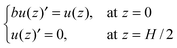
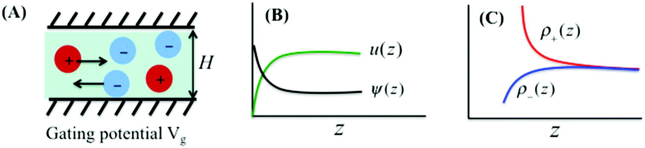
We consider ionic transport through a nanochannel for a simple electrolyte consisting of spherical ions. Approximately, the model system mimics a typical experimental setup for electroosmotic flow under steady-state conditions. The nanochannel has width H on the nanoscale and the other dimensions, L and W, on macroscopic scales, resembling a slit pore. Fig. 1 schematically shows the ion flow through the nanopore induced by a uniform electric field, Ex = V/L, with V being the electric potential in the x-direction, i.e., the direction along the pore length L. The gating voltage Vg is fixed at the pore surface (or the surface of a porous material). In electroosmotic flows, the electrical current arises from ionic motions through the charged nanochannel driven by the external field Ex. While the flow in the x-direction is induced by the external driving force, it is conventionally assumed that the ion distribution in the z-direction is the same as that at equilibrium since there is no current flowing through the walls.
 |
| | Fig. 1 (A) Electroosmotic flow through a nanopore of width H and gating voltage Vg. (B and C) Variations of local electrical potential ψ(z), solvent velocity u(z), and ionic densities ρ±(z) throughout the nanopore, where z represents the distance from the wall. While the Donnan model assumes uniform electric potential and ionic density profiles, we account for the local inhomogeneity through the DFT–NS equations. | |
Ionic transport through a nanopore is typically measured in terms of the conductance, G = I/V, i.e., ionic current I divided by voltage drop V. A conventional model to describe the conductance is based on the Donnan equilibrium, which assumes uniform ionic densities inside the pore. For systems containing symmetric monovalent ions, the Donnan model (DM) yields an analytical expression for the conductance as a function of surface charge density Q and bulk salt concentration ρs27,43
| |  | (1) |
where
ν stands for the mean ionic mobility and
e is the proton charge. According to
eqn (1), the conductance scales
G ∼
Q at low salt concentrations and
G ∼
Hρs when
ρs ≫
Q/
H. Whereas the scaling predictions appear robust for ionic transport in highly charged pores,
27,49,50 its validity becomes questionable at both low and high concentrations when the pore size is comparable to the EDL thickness, in particular if the surface is only weakly charged.
51
To have a more comprehensive description of the conductance, we follow a modified space-charge model that accounts for inhomogeneous ion concentrations and solvent velocity inside the pore.52 As in a previous work,17 we adopt the restricted primitive model to represent the ionic species in which the solvent is represented as a dielectric continuum and the ions as charged hard spheres of equal size. We take the ion diameter of 0.5 nm for all hydrated monovalent ions, approximately corresponding to those ionic species in aqueous NaCl solutions.53 At ambient temperature, the dielectric constant for liquid water is εr = 78.4. Different from the conventional space-charge model, we use the classical DFT to describe inhomogeneous ion distributions. For ionic species in a slit pore, the ionic density profiles vary in the z-direction, i.e., perpendicular from the wall54
| | ρi(z) = ρbulki![[thin space (1/6-em)]](https://www.rsc.org/images/entities/char_2009.gif) exp[−βZieψ(z) − βΔμexi(z)] exp[−βZieψ(z) − βΔμexi(z)] | (2) |
where
ρbulki represents the bulk concentration of ion
i,
β = (
kBT)
−1,
kB is the Boltzmann constant,
T = 298 K,
Zi = ±1 denotes the ion valence,
ψ(
z) represents the local electric potential, and Δ
μexi(
z) stands for the deviation of the local excess chemical potential for ionic species
i from that in the bulk solution. Without the local excess chemical potential,
eqn (2) reduces to the Poisson–Boltzmann (PB) equation, which is used in the conventional space-charge model. As in our previous work for equilibrium electrolyte systems, the local excess chemical potential includes a contribution from the modified fundamental measure theory (MFMT)
55 to account for ionic size and a second-order perturbation theory for electrostatic correlations.
56 The theoretical performance for the classical DFT has been repeatedly calibrated with molecular simulations.
54,56–58 The detailed expression for the excess chemical potential can be found in the ESI.
†
The electric potential satisfies the Poisson equation
| | 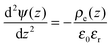 | (3) |
where
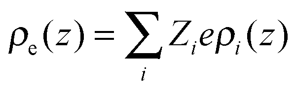
ε0 is the vacuum permittivity and
stands for the local charge density.
Eqn (2) and (3) can be solved self-consistently with the following boundary conditions
Throughout this work, we assume that the gating potential is always positive,
Vg > 0. Because cations and anions have the same size but opposite charges in our model, the ionic conductance would be the same if the gating potential changes from positive to negative.
To relate the gating potential with the surface charge density, we follow the Gauss law assuming no electric field outside the pore (i.e., metallic electrodes):
| |  | (5) |
Because of the plane symmetry of a slit pore,
, and the derivative of the electrostatic potential at the wall can be calculated by integrating
eqn (3).| |  | (6) |
Eqn (6) suggests that the charge neutrality is always satisfied for all ionic systems confined between metallic walls:
| |  | (7) |
From the ionic density profiles, we can also obtain the velocity profile of the solvent by solving the Navier–Stokes (NS) equation.
where
u is the solvent velocity in the
x direction and
η is the solvent viscosity. The boundary conditions for the NS equation are
| |  | (9) |
where
b stands for the slip length. According to a previous study,
27 the slip length takes a negative value for water flowing through a hydrophilic pore and positive if the surface is hydrophobic. In this work,
b = 0 is used for all results discussed in the following. As a result, we find from
eqn (3) and (8) that the solvent velocity is linearly related to the electric potential:
Eqn (10) indicates that the maximum solvent velocity appears at the pore center where the difference between the local and the surface electrical potentials is the largest. Although the local electrical potential
ψ is highly inhomogeneous when the pore size is comparable to the ion diameters, the solvent velocity at the pore center rises smoothly to its asymptotic value
u∞ =
ε0εrExVg/
η for large pores (Fig. S1 and S2, ESI
†). Because the Donnan model assumes a constant electric potential throughout the pore, it predicts erroneously zero solvent velocity.
The ion velocities inside the pore, ui(z), can be calculated from a superposition of the solvent velocity, u(z), and the ion motion due to the external electrical field.
| | | ui(z) = u(z) − eZiνiEx | (11) |
where
νi represents the ion mobility. For electrolytes considered in this work, we assume
ν =
ν+ =
ν− = 4.8 × 10
11 s kg
−1, corresponding to the mean value of Na
+ and Cl
− ions in an aqueous solution. With the inhomogeneous ionic distributions and the ion velocity profile inside the pore obtained from the classical DFT and the NS equations, we can now calculate the electrical current
27| | 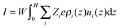 | (12) |
Theoretical predictions of the DFT–NS equations have been validated in our previous work for ion transport in boron nitride nanopores.
17 It has been shown that the DFT–NS model agrees well with experimental data, while the conventional space-charge model overpredicts the surface charge density and conductance.
III. Results and discussion
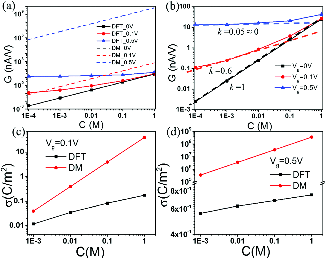
For all theoretical results discussed in this work, we specify the surface voltage instead of the surface charge density of nanopores. At a given surface electrical potential, the local ionic concentrations and, subsequently, the ionic transport in the nanopore are independent of the dielectric details of the solid material. Furthermore, the continuous model ignores non-electrostatic effects such as the surface hydrophobicity on ion distributions and the local solvent velocity. Fig. 2(a) compares conductance G calculated from the Donnan method (DM) and that from the DFT–NS equations at different salt concentrations. Here three representative gating voltages are considered, corresponding to neutral, low and high values used in experiments.59,60 To mimic the experimental conditions, we fix the driving voltage, V = 2.0 V; the length of the slit pore is L = 900 nm; and the slit pore width H is 30 nm. The DM and DFT–NS predictions are virtually identical at zero gating voltage. When the gating voltage is low (0.1 V), the DM and DFT–NS methods predict similar conductance at low salt concentrations but significant discrepancy is observed as the salt concentration increases. At a large gating voltage (0.5 V), the DM method overpredicts the conductance by several orders of magnitude at all concentrations.
 |
| | Fig. 2 (a) Conductance vs. salt concentration at different gating voltages. (b) The scaling behavior of conductance according to the DFT–NS predictions. Surface charge density σ predicted by the DFT and DM methods at gating voltage (c) Vg = 0.1 V, and (d) Vg = 0.5 V. | |
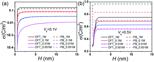
Fig. 2(b) shows the conductance predicted by the DFT–NS equations at different gating voltages. Previous work on ion transport in weakly charged nanopores such as carbon nanotubes (CNTs) suggests that the conductance exhibit a power law behavior at low salt concentrations, with an exponent close to 1/3 versus the salt concentration,21,51 which contradicts with ion transport in boron nitride or silica nanopores that exhibit a conductance independent of salt concentration.10,43 According to Fig. 2(b), the scaling exponent at low salt concentration depends on the gating voltage; the slope falls from 1 to 0 as the gating voltage increases from 0 to 0.5 V. Without the gating voltage, the surface charge density vanishes because all ionic species have the same size and absolute charge, thus the potential of zero charge (PZC) is zero. In this case, the conductance depends linearly on the salt concentration, as shown by the black-dashed line in Fig. 2(b). Fig. 2(c) and (d) compare the surface charge densities predicted by the DM and DFT–NS methods. At a small gating potential (0.1 V), the DM and DFT–NS predictions are on the same order of magnitude albeit the gap increases as the salt concentration increases. Approximately, the surface charge density varies with the salt concentration as σ ∼ C1/3, in excellent agreement with recent experiments and scaling analysis.51 At a large gating potential (0.5 V), however, the surface charge predicted by the DM model is larger than that from the DFT–NS equations again by several orders of magnitude. In this case, the surface charge density varies little with the bulk salt concentration, indicating that the scaling analysis becomes inadequate at high gating potentials.
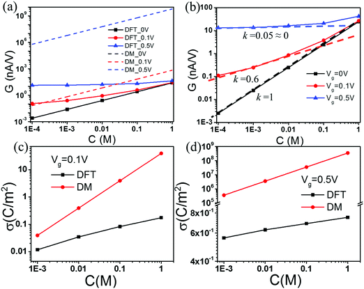
Fig. 3 shows the effect of the nanopore size (H) on conductance G at various salt concentrations. For comparison between different methods, the results from both the DM (dashed lines) and the DFT–NS equations (solid lines) are presented in Fig. 3(a) and (b), and those from the DFT–NS (solid lines) and the PB–NS equations (dashed lines) are shown in Fig. 3(c) and (d), respectively. Because the electric potential inside the pore is assumed to be the same as the gating potential, the DM predictions are significantly larger than those from DFT–ND equations. Nevertheless, both methods predict that the conductance increases with pore size, primarily due to the increased cross-section area. The DFT and PB equations yield similar results at small salt concentrations and low gating voltages. Both equations predict that an increase in salt concentration or gating voltage leads to a higher surface charge density. Fig. 3(d) shows that, in comparison to the classical DFT, the PB equation overpredicts the electrical conductance at high gating voltages, and the discrepancy increases at high salt concentrations. Such a difference can be attributed to the EDL structure near a highly charged surface, which is sensitive to the ionic excluded volume effects and electrostatic correlations. While thermodynamic non-ideality is faithfully described by the classical DFT, it is only partially captured by the PB equation.61,62 In particular, neglecting the ionic excluded volume effects and electrostatic correlations results in significant overestimation of the electrical conductance, especially for nanopores with a small pore size and at a high salt concentration.
 |
| | Fig. 3 Electrical conductance G vs. pore size H at various salt concentrations. Here the gating voltage is Vg = 0.1 V for (a) and (c), and 0.5 V for (b) and (d). The comparison between DM and DFT–NS predictions is shown in (a) and (b), and that between PB and DFT equations in (c) and (d). | |
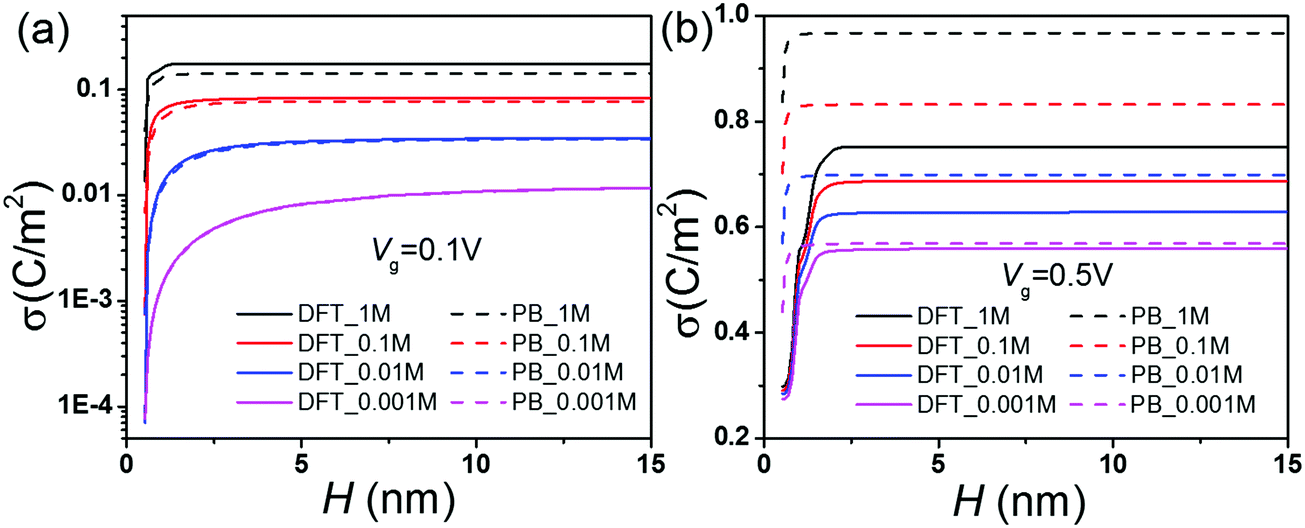
Fig. 4 shows that the surface charge density reaches an asymptotic value when the pore width is sufficiently large. The asymptotic charge density corresponds to that of a single wall, depending on the bulk salt concentration Cb and the gating voltage Vg. For large pores, the electric double layers at the opposite sides are uncorrelated. As a result, the conductance scales linearly with the pore size and the bulk concentration. While Fig. 3 shows good consistency with the scaling relation and the DFT–NS predictions for large pores, we see no simple linear correlation for small channels (0.5 nm to 2.5 nm). In this region, the surface charge density increases sharply when the pore size increases (Fig. 4). As the pore size increases, the surge in conductance is attributed not only to the larger cross-section area but also to the higher solvent velocity inside the nanochannel (Fig. S1 and S2, ESI†). At a low salt concentration or a large gating potential, the overlapping EDLs inside small pores play an important role in determining the surface charge density and the solvent velocity. As shown in Fig. 4, the discrepancy between the DFT and PB equations is most significant for a small pore with a large gating voltage, implying a significant difference in their prediction of the EDL overlap. When the gating voltage is small (0.1 V), the increase of the bulk salt concentration leads to a drastic increase of the surface charge density and the conductance by almost several orders of magnitude. However, the changes are relatively modest at a high gating voltage (0.5 B).
 |
| | Fig. 4 Surface charge density σ vs. pore size H at various salt concentrations. | |
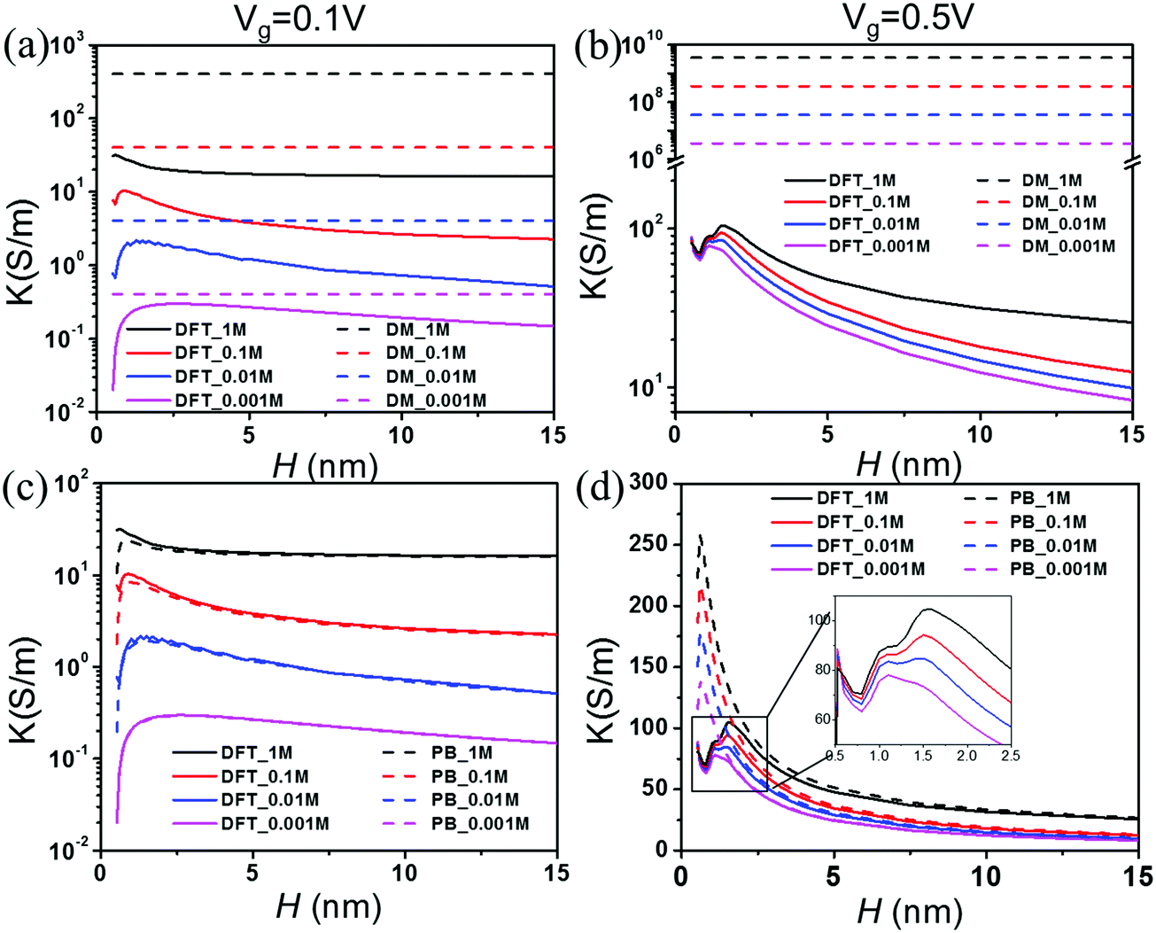
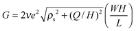
Fig. 5 presents the theoretical predictions of the electrical conductivity, defined as K ≡ GL/(WH), as a function of the pore size at different salt concentrations and two gating voltages. According to the Donnan equilibrium, the surface charge density divided by the pore width depends only on the gating potential and the salt bulk concentration
| | | σ/H = −ρssinh(βeVg) | (13) |
Substituting
eqn (13) into
(1) yields.
| | | K = 2νe2ρscosh(βeVg). | (14) |
Eqn (14) predicts that, at a given surface potential
ψs, the conductivity scales linearly with ion mobility
ν and bulk salt concentration
ρs, in dependent of the pore size. According to the DFT–NS equations, the conductance is relatively insensitive to the pore size for large pores with a small gating voltage (
Vg = 0.1 V), which agrees reasonably well with the Donnan model. At a large gating potential (0.5), however, the results are qualitatively different.
Fig. 5(b) shows that the conductivity declines with the pore width at separations even after the surface charge reaches its asymptotic limit.
Fig. 5(c) and (d) compare the conductivities predicted from the PB and DFT equations. When the gating voltage is small (0.1 V), the PB and DFT equations yield similar results; both show a maximum conductivity at
H = 1–2 nm. At higher gating voltages, the difference between the DFT and PB predictions is mainly manifested for small pores. While the PB equation predicts a smooth variation of the conductivity, DFT predicts that the conductivity oscillates due to the significant overlap of EDLs and that the maximum conductivity appears at about 2 nm before its fall-off at a larger pore width. As shown in the inset of
Fig. 5(d), the conductivity reduces from over 100 S m
−1 at the peak value to about 70 S m
−1 at its minimum when the pore size is reduced from 1.8 nm to 0.7 nm. The reduction of the conductivity is significant from the perspective of pore size optimization because it is comparable to the corresponding asymptotic value for macroscopic pores (∼25 S m
−1).
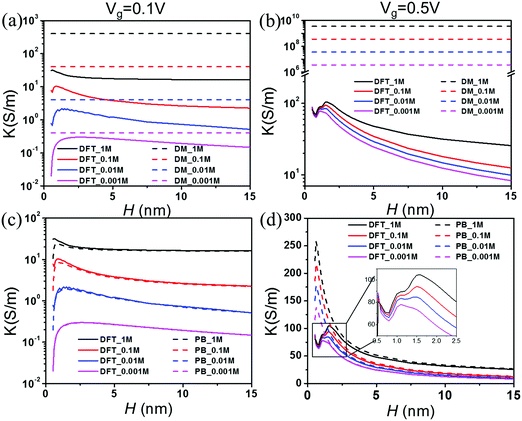 |
| | Fig. 5 Conductivity K vs. pore size H at various salt concentrations. The gating voltage is Vg = 0.1 V for (a) and (c) and 0.5 V for (b) and (d). | |
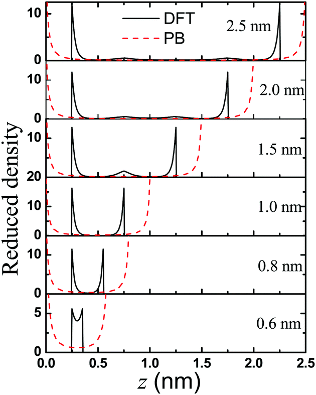
What are the causes of the oscillatory dependence of the conductivity on the pore size? Why does the nanopore show a maximum conductivity? To understand the behavior of the three peaks in the K–H curves, we present the density profiles of counterions inside the nanopores in Fig. 6. For ions in a highly charged nanopore, the EDL structure is dominated by the distribution of counterions. Clearly, the classical DFT and PB equations predict different trends on the effect of the pore size on the counterion distribution. While the PB equation predicts a concave up density profile inside the pore regardless of the pore size, the classical DFT predicts that the density profiles near a highly charged surface are non-monotonic. We see a second layer of counterions near the surface of a large pore (e.g., 2.5 nm and 2.0 nm in Fig. 6). The layering effects reflect the electrostatic correlations and ionic excluded volume effects that are ignored in the PB equation. According to the DFT predictions, the second layer near each surface will overlap when the pore size decreases, as shown in Fig. 6. By contrast, the PB equation is unable to reproduce the layering effects since the ionic excluded volume is neglected, and thus it predicts no oscillatory dependence of the conductivity on the pore size. To our best knowledge, this pore-size dependent oscillatory behavior of conductivity K at the high surface charge density has never been reported before.
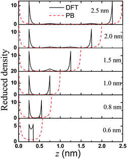 |
| | Fig. 6 Anion distribution in the nanochannels with width varying from H = 2.5 to 0.6 nm. Here the gating voltage is fixed at 0.5 V. | |
IV. Conclusions
In conclusion, we have studied ionic transport through voltage-gated nanopores using the classical density functional theory (DFT) and the Navier–Stokes (NS) equation. Unlike conventional methods based on the Donnan equilibrium or the Poisson–Boltzmann equation, the classical DFT accounts for ion excluded volume effects and electrostatic correlations important for ionic systems in small pores. We elucidate, for the first time, the effects of the pore size and the gating potential of nanochannels on electrical conductivity at different salt concentrations. In addition to identifying the oscillatory dependence of conductivity on the pore size, we find that the conductance varies in response to changes in pore size and salt concentration qualitatively different from the conventional scaling predictions but in good agreement with recent experiments. The theoretical results reconcile a longstanding controversy over how conductance varies with the salt concentration for weakly charged nanochannels. We hope that this work will inspire future experiments or more detailed all-atom molecular dynamics simulations to confirm our theoretical predictions.
Acknowledgements
This research was sponsored by the Fluid Interface Reactions, Structures and Transport (FIRST) Center, an Energy Frontier Research Center funded by the U.S. Department of Energy, Office of Science, Office of Basic Energy Sciences. Cheng Lian and Honglai Liu thank the financial support by the National Natural Science Foundation of China (No. 91334203) and the 111 Project of China (No. B08021). Cheng Lian is also grateful to the Chinese Scholarship Council for the visiting fellowship. The numerical calculations were performed at the National Energy Research Scientific Computing Center (NERSC).
References
- A. R. Koltonow and J. Huang, Science, 2016, 351, 1395–1396 CrossRef CAS PubMed.
- C. Cheng, G. Jiang, C. J. Garvey, Y. Wang, G. P. Simon, J. Z. Liu and D. Li, Sci. Adv., 2016, 2, e1501272 CrossRef PubMed.
- Z. Zhang, X.-Y. Kong, K. Xiao, Q. Liu, G. Xie, P. Li, J. Ma, Y. Tian, L. Wen and L. Jiang, J. Am. Chem. Soc., 2015, 137, 14765–14772 CrossRef CAS PubMed.
- Z. Zhang, X. Y. Kong, K. Xiao, G. Xie, Q. Liu, Y. Tian, H. Zhang, J. Ma, L. Wen and L. Jiang, Adv. Mater., 2016, 28, 144–150 CrossRef CAS PubMed.
- K. Raidongia and J. Huang, J. Am. Chem. Soc., 2012, 134, 16528–16531 CrossRef CAS PubMed.
- Y. Zhu, Y. Ruan, Y. Zhang, L. Lu and X. Lu, Mol. Simul., 2016, 42, 784–798 CrossRef CAS.
- J. Li, X. Kong, D. Lu and Z. Liu, Sci. Bull., 2015, 60, 1580–1586 CrossRef CAS.
- J. Gao, W. Guo, D. Feng, H. Wang, D. Zhao and L. Jiang, J. Am. Chem. Soc., 2014, 136, 12265–12272 CrossRef CAS PubMed.
- W. Sparreboom, A. Van Den Berg and J. Eijkel, Nat. Nanotechnol., 2009, 4, 713–720 CrossRef CAS PubMed.
- A. Siria, P. Poncharal, A.-L. Biance, R. Fulcrand, X. Blase, S. T. Purcell and L. Bocquet, Nature, 2013, 494, 455–458 CrossRef CAS PubMed.
- H. Liu, J. He, J. Tang, H. Liu, P. Pang, D. Cao, P. Krstic, S. Joseph, S. Lindsay and C. Nuckolls, Science, 2010, 327, 64–67 CrossRef CAS PubMed.
- J. Li, M. Gershow, D. Stein, E. Brandin and J. Golovchenko, Nat. Mater., 2003, 2, 611–615 CrossRef CAS PubMed.
- R. Joshi, P. Carbone, F. Wang, V. Kravets, Y. Su, I. Grigorieva, H. Wu, A. Geim and R. Nair, Science, 2014, 343, 752–754 CrossRef CAS PubMed.
- D. Gillespie and S. Pennathur, Anal. Chem., 2013, 85, 2991–2998 CrossRef CAS PubMed.
- Z.-X. Luo, Y.-Z. Xing, Y.-C. Ling, A. Kleinhammes and Y. Wu, Nat. Commun., 2015, 6, 6358 CrossRef CAS PubMed.
- T. Colla, M. Girotto, A. P. Santos and Y. Levin, J. Chem. Phys., 2016, 145, 094704 CrossRef PubMed.
- X. Kong, J. Jiang, D. Lu, Z. Liu and J. Wu, J. Phys. Chem. Lett., 2014, 5, 3015–3020 CrossRef CAS PubMed.
- D. Gillespie, Nano Lett., 2012, 12, 1410–1416 CrossRef CAS PubMed.
- L. H. Yeh, M. K. Zhang and S. Z. Qian, Anal. Chem., 2013, 85, 7527–7534 CrossRef CAS PubMed.
- Z. Zeng, L.-H. Yeh, M. Zhang and S. Qian, Nanoscale, 2015, 7, 17020–17029 RSC.
- P. Pang, J. He, J. H. Park, P. S. Krstic and S. Lindsay, ACS Nano, 2011, 5, 7277–7283 CrossRef CAS PubMed.
- F. H. J. van der Heyden, D. Stein, K. Besteman, S. G. Lemay and C. Dekker, Phys. Rev. Lett., 2006, 96, 224502 CrossRef PubMed.
- C. Duan and A. Majumdar, Nat. Nanotechnol., 2010, 5, 848–852 CrossRef CAS PubMed.
- D. J. Bonthuis, S. Gekle and R. R. Netz, Phys. Rev. Lett., 2011, 107, 166102 CrossRef PubMed.
- D. J. Bonthuis and R. R. Netz, Langmuir, 2012, 28, 16049–16059 CrossRef CAS PubMed.
- Y. Ma, L.-H. Yeh, C.-Y. Lin, L. Mei and S. Qian, Anal. Chem., 2015, 87, 4508–4514 CrossRef CAS PubMed.
- L. Bocquet and E. Charlaix, Chem. Soc. Rev., 2010, 39, 1073–1095 RSC.
- Y. Qiao, B. Tu and B. Lu, J. Chem. Phys., 2014, 140, 174102 CrossRef PubMed.
- J. Hoffmann and D. Gillespie, Langmuir, 2013, 29, 1303–1317 CrossRef CAS PubMed.
- D. Gillespie, Microfluid. Nanofluid., 2015, 18, 717–738 CrossRef CAS.
- M. Z. Bazant, B. D. Storey and A. A. Kornyshev, Phys. Rev. Lett., 2011, 106, 046102 CrossRef PubMed.
- B. D. Storey and M. Z. Bazant, Phys. Rev. E, 2012, 86, 056303 CrossRef PubMed.
- R. F. Stout and A. S. Khair, J. Fluid Mech., 2014, 752, R1 CrossRef CAS.
- Y. Xin, Y.-X. Zheng and Y.-X. Yu, Mol. Phys., 2016, 114, 2328–2336 CrossRef CAS.
- F. Baldessari, J. Colloid Interface Sci., 2008, 325, 526–538 CrossRef CAS PubMed.
- L.-H. Yeh, Y. Ma, S. Xue and S. Qian, Sens. Actuators, B, 2015, 215, 266–271 CrossRef CAS.
- R. H. Nilson and S. K. Griffiths, J. Chem. Phys., 2006, 125, 164510 CrossRef PubMed.
- R. Toghraee, R. J. Mashl, K. I. Lee, E. Jakobsson and U. Ravaioli, J. Comput. Electron., 2009, 8, 98–109 CrossRef CAS PubMed.
- M. M. Hatlo, R. Van Roij and L. Lue, EPL, 2012, 97, 28010 CrossRef.
- M. Wang, C.-C. Chang and R.-J. Yang, J. Chem. Phys., 2010, 132, 024701 CrossRef PubMed.
- W.-L. Hsu, H. Daiguji, D. E. Dunstan, M. R. Davidson and D. J. E. Harvie, Adv. Colloid Interface Sci., 2016, 234, 108–131 CrossRef CAS PubMed.
- H. Daiguji, P. Yang, A. J. Szeri and A. Majumdar, Nano Lett., 2004, 4, 2315–2321 CrossRef CAS.
- D. Stein, M. Kruithof and C. Dekker, Phys. Rev. Lett., 2004, 93, 035901 CrossRef PubMed.
- R. Fan, S. Huh, R. Yan, J. Arnold and P. D. Yang, Nat. Mater., 2008, 7, 303–307 CrossRef CAS PubMed.
- S. Bearden, E. Simpanen and G. Zhang, Nanotechnology, 2015, 26, 185502 CrossRef PubMed.
- S. Mafe, J. A. Manzanares and P. Ramirez, J. Phys. Chem. C, 2010, 114, 21287–21290 CrossRef CAS.
- S. Bearden, E. Simpanen and G. Zhang, Nanotechnology, 2016, 27, 075503 CrossRef PubMed.
- T. James, Y. V. Kalinin, C.-C. Chan, J. S. Randhawa, M. Gaevski and D. H. Gracias, Nano Lett., 2012, 12, 3437–3442 CrossRef CAS PubMed.
- R. B. Schoch, J. Y. Han and P. Renaud, Rev. Mod. Phys., 2008, 80, 839–883 CrossRef CAS.
- H. C. Chang, G. Yossifon and E. A. Demekhin, Annu. Rev. Fluid Mech., 2012, 44, 401–426 CrossRef.
- E. Secchi, A. Niguès, L. Jubin, A. Siria and L. Bocquet, Phys. Rev. Lett., 2016, 116, 154501 CrossRef PubMed.
- P. B. Peters, R. van Roij, M. Z. Bazant and P. M. Biesheuvel, Phys. Rev. E, 2016, 93, 053108 CrossRef CAS PubMed.
- J. G. Ibarra-Armenta, A. Martin-Molina and M. Quesada-Perez, Phys. Chem. Chem. Phys., 2011, 13, 13349–13357 RSC.
- Z. D. Li and J. Z. Wu, J. Phys. Chem. B, 2006, 110, 7473–7484 CrossRef CAS PubMed.
- Y. X. Yu and J. Z. Wu, J. Chem. Phys., 2002, 117, 10156–10164 CrossRef CAS.
- Y. X. Yu, J. Z. Wu and G. H. Gao, Chin. J. Chem. Eng., 2004, 12, 688–695 CAS.
- C. Lian, D.-e. Jiang, H. Liu and J. Wu, J. Phys. Chem. C, 2016, 120, 8704–8710 CrossRef CAS.
- C. Lian, K. Liu, K. L. Van Aken, Y. Gogotsi, D. J. Wesolowski, H. L. Liu, D. E. Jiang and J. Z. Wu, ACS Energy Lett., 2016, 1, 21–26 CrossRef CAS.
- S.-W. Nam, M. J. Rooks, K.-B. Kim and S. M. Rossnagel, Nano Lett., 2009, 9, 2044–2048 CrossRef CAS PubMed.
- J. Goldberger, R. Fan and P. Yang, Acc. Chem. Res., 2006, 39, 239–248 CrossRef CAS PubMed.
- L. Mier-y-Teran, S. H. Suh, H. S. White and H. T. Davis, J. Chem. Phys., 1990, 92, 5087–5098 CrossRef CAS.
- Y. X. Yu, J. Z. Wu and G. H. Gao, J. Chem. Phys., 2004, 120, 7223–7233 CrossRef CAS PubMed.
Footnotes |
| † Electronic supplementary information (ESI) available. See DOI: 10.1039/c6cp07124d |
| ‡ These authors made equal contribution to this work. |
|
| This journal is © the Owner Societies 2017 |
Click here to see how this site uses Cookies. View our privacy policy here. 


 stands for the local charge density. Eqn (2) and (3) can be solved self-consistently with the following boundary conditions
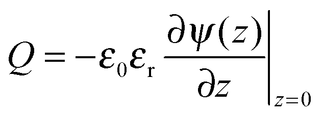
 , and the derivative of the electrostatic potential at the wall can be calculated by integrating eqn (3).