
 Open Access Article
 This Open Access Article is licensed under a
 Creative Commons Attribution 3.0 Unported Licence
Phase separation and coexistence of hydrodynamically interacting microswimmers†
Johannes
Blaschke
 *a,
Maurice
Maurer
b,
Karthik
Menon
a,
Andreas
Zöttl
c and
Holger
Stark
*a
*a,
Maurice
Maurer
b,
Karthik
Menon
a,
Andreas
Zöttl
c and
Holger
Stark
*a
aInstitute of Theoretical Physics, Technische Universität Berlin, Hardenbergstr. 36, D-10623 Berlin, Germany. E-mail: johannes.blaschke@tu-berlin.de; holger.stark@tu-berlin.de
bDepartment of Physics and Astronomy, University of California, Los Angeles, California 90095, USA
cThe Rudolf Peierls Centre for Theoretical Physics, University of Oxford, 1 Keble Road, Oxford, OX1 3NP, UK
First published on 14th November 2016
Abstract
A striking feature of the collective behavior of spherical microswimmers is that for sufficiently strong self-propulsion they phase-separate into a dense cluster coexisting with a low-density disordered surrounding. Extending our previous work, we use the squirmer as a model swimmer and the particle-based simulation method of multi-particle collision dynamics to explore the influence of hydrodynamics on their phase behavior in a quasi-two-dimensional geometry. The coarsening dynamics towards the phase-separated state is diffusive in an intermediate time regime followed by a final ballistic compactification of the dense cluster. We determine the binodal lines in a phase diagram of Péclet number versus density. Interestingly, the gas binodals are shifted to smaller densities for increasing mean density or dense-cluster size, which we explain using a recently introduced pressure balance [S. C. Takatori, et al., Phys. Rev. Lett. 2014, 113, 028103] extended by a hydrodynamic contribution. Furthermore, we find that for pushers and pullers the binodal line is shifted to larger Péclet numbers compared to neutral squirmers. Finally, when lowering the Péclet number, the dense phase transforms from a hexagonal “solid” to a disordered “fluid” state.
1 Introduction
Collective dynamics due to the active motion of microorganisms and artificial microswimmers has received a lot of attention among physicists1–6 as it is relevant both to real world applications2,6–8 as well as for posing fundamental questions in non-equilibrium statistical physics.4,9–13 From the perspective of physics, a unifying feature of microorganisms and artificial microswimmers is that they propel themselves autonomously through a surrounding fluid. As they are constantly driven out of equilibrium, understanding the collective properties of systems comprised of many swimmers is an important field of ongoing research in statistical physics.One of the most striking features of swimmer systems is motility-induced phase separation,14 where stable clusters of swimmers form due to their active motion alone and without any attractive forces. The question of motility-induced phase separation has been treated theoretically using so-called active Brownian particles, which perform a persistent random walk and interact sterically only.11,15–19 However, real microswimmers such as ciliated microorganisms,20 catalytic Janus particles,7,8,21–23 or active emulsion droplets2,24–27 employ propulsion mechanisms reliant on hydrodynamics. Thus nearby microswimmers can affect each other's velocity and orientation, which can potentially alter their collective behaviour depending on the details of their hydrodynamic interactions.28
Biological microswimmers employ non-reciprocal cell-body deformations or the collective dynamics of flagella or cilia in order to propel themselves,29 whereas active colloids and droplets move forward by creating a slip velocity close to their surface.1 The essential features of both of these self-propulsion mechanisms are captured by the so-called “squirmer” model,30–34 which we shall use to generate our hydrodynamic propulsion.
For phase separating systems, it is common to construct the binodal line in order to determine the phase coexistence region. While there have been many studies quantifying the phase-coexistence regime for active Brownian particles,11,13,15,35–38 to list just a few of them, none of these have considered hydrodynamic interactions between the swimmers. Several recent works studied the collective dynamics of hydrodynamic swimmers,39–43 but did not look at phase separation.
In our previous study, we examined the collective dynamics and clustering of hydrodynamic squirmers in a quasi-two-dimensional geometry using the method of multi-particle collision dynamics (MPCD) to explicitly simulate the fluid environment.28 Due to computational limitations, we were restricted to 208 swimmers, which was insufficient to quantify the first-order phase-separation transition. Hence, we built on this study and extended the simulations to thousands of squirmers by implementing a parallelized version on 1008 processor cores. This allows us to investigate the dynamics of a sufficiently large number of squirmers in order to quantitatively resolve phase separation into a dilute gas and a dense phase.
In the following we show phase-separated squirmer systems and explain how we analyze them to obtain the area fractions of the dilute and dense phases. After illustrating the coarsening dynamics towards phase separation, we quantify the coexistence region bounded by the binodal line in a diagram Péclet number versus density. Interestingly, the binodal lines differ for varying mean density. We explain this phenomenon as a true hydrodynamic signature using a pressure balance. In particular, we use the swim pressure introduced in ref. 9 and extend the approach of ref. 9 and 10 by including a hydrodynamic pressure generated by squirmers at the rim of the dense cluster. The binodal line is shifted towards larger Péclet numbers, when the force-dipole contribution of the squirmer, characterizing pushers and pullers, is increased. Finally, moving the dense phase from large Péclet numbers to the critical value, one observes a melting transition between a hexagonal and a fluid phase. We start with summarizing computational details.
2 System and methods
Our system consists for N spherical squirmers of radius R, where N varies from 2116 to 4900 depending on mean area fraction or density![[small phi, Greek, macron]](https://www.rsc.org/images/entities/i_char_e0d6.gif) . Squirmers propel themselves by applying an axisymmetric surface-velocity field,33,34
. Squirmers propel themselves by applying an axisymmetric surface-velocity field,33,34vs = B1(1 + βê·![[r with combining circumflex]](https://www.rsc.org/images/entities/b_char_0072_0302.gif) s)[(ê·s)s − ê] s)[(ê·s)s − ê] | (1) |
s is the unit vector along rs, and ê is the squirmer's orientation. The constant B1 determines the amplitude of the slip velocity and thus its swimming speed v0. For a single squirmer in a bulk fluid, v0 = 2B1/3. We use B1 to control the Péclet number, Pe = Rv0/DT, as the appropriate thermal diffusion coefficient DT is kept constant for all simulations. For the MPCD fluid and squirmer parameters presented below, we obtain Pe ≈ 3546.4B1. The additional parameter β breaks the symmetry about the squirmer equator. For β < 0, the surface field is more concentrated on the southern hemisphere and the squirmer's far field in bulk is that of a pusher. For β > 0 a puller is realized and a swimmer with β = 0 is called a “neutral squirmer”.
Motivated by experiments2,24,44 and following our previous study,28 the swimmers are bounded by two parallel flat plates. As in ref. 28 we choose strong confinement with the distance between the plates being H = 8R/3. We implement the full hydrodynamic interactions between squirmers and confining walls using the MPCD simulation technique.45,46 The fluid is represented by of the order of 107 point-like effective fluid particles with mass m0, velocity vi(t), and position ri(t). The velocities vi(t) are thermostatted to have a temperature T0. The fluid particles perform alternating streaming and collision steps. During the streaming step, fluid particles move ballistically over a time Δt without interacting with each other and reach the position
| ri(t + Δt) = ri + vi(t)Δt. | (2) |
![[v with combining macron]](https://www.rsc.org/images/entities/b_char_0076_0304.gif) = 〈vi〉cell and centre of mass
= 〈vi〉cell and centre of mass ![[r with combining macron]](https://www.rsc.org/images/entities/b_char_0072_0304.gif) = 〈ri〉cell of the particles in each cell is determined. Within each cell they “collide” according to the MPCD-AT+a rule,45 which is reminiscent of an Andersen thermostat and also conserves linear and angular momentum. Random velocity increments δvi for each particle are sampled from a Gaussian distribution with variance kBT0/m0. The velocity increments would give an overall change in momentum m0Δ = m0〈δvi〉cell and angular momentum ΔL = m0〈(ri − ) × δvi〉cell. Hence, we subtract these changes in the velocity increment for the collision step,
= 〈ri〉cell of the particles in each cell is determined. Within each cell they “collide” according to the MPCD-AT+a rule,45 which is reminiscent of an Andersen thermostat and also conserves linear and angular momentum. Random velocity increments δvi for each particle are sampled from a Gaussian distribution with variance kBT0/m0. The velocity increments would give an overall change in momentum m0Δ = m0〈δvi〉cell and angular momentum ΔL = m0〈(ri − ) × δvi〉cell. Hence, we subtract these changes in the velocity increment for the collision step,| vi(t + Δt) = (t) + δvi − Δ − (ri(t) − (t)) × I−1ΔL, | (3) |
2.1 System parameters
For all simulations discussed here, the fluid and squirmer mass densities are the same, ρ = 10m0/a03, and the squirmer radius is R = 3a0. Together with the streaming-time step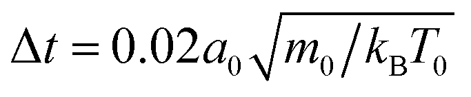 , the fluid viscosity becomes
 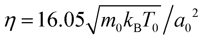 taken from ref. 28 and 48. For the bulk fluid and the parameters stated above, the self-diffusivity of a passive colloid is
 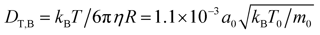 . In the presence of walls, the self-diffusivity becomes a position-dependent tensor.51 We measure the self-diffusivity at the centre between the walls using the Green–Kubo formula. We find that DT,2D ≈ 0.5DT,B, comparable to the result of ref. 51. For a colloid close to the walls this value can decrease to approximately 0.25DT,B due to the enhanced friction. In the following, we use DT,2D for a single particle (particle density ϕ = 0) to define the Péclet number,
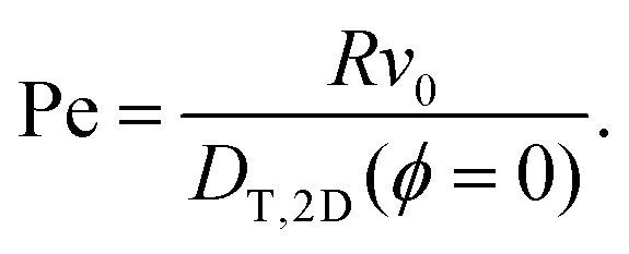 | (4) |
The orientation of a squirmer also undergoes rotational diffusion, for which MPCD gives the rotational diffusion coefficient  in a bulk fluid, which is also approximately valid in our quasi-two-dimensional geometry. There, rotational diffusion strongly depends on the density of squirmers due to the flow field they create and increases by as much as a factor of 15 in very dense systems.28 The rotational diffusion coefficient is used to define the persistence number Per = v0/RDR, which compares persistence or run length l = v0/DR to R.
To summarise, in the following we work with Péclet numbers in the range [190, 355], which corresponds to persistence numbers Per in the range [120, 220] or typical run lengths of single squirmers, l = v0/DR, ranging from 120R to 220R. For high-density simulations without phase separation, where rotational diffusion is considerably enhanced, we have Per ≳ 8 or l ≳ 8R.
3 Results
3.1 Phase separation and coarsening dynamics
For a range of total densities and Péclet numbers, the system decomposes into a dilute gas and a dense phase. Fig. 1: top, left shows a typical snapshot of a phase-separated system with mean area fraction = 0.64 and at Péclet number Pe = 355 (B1 = 0.1). The two phases are clearly visible: many squirmers have come together to form a densely packed and system-spanning cluster, leaving a few squirmers in a much less dense “gas” phase. For lower , the dense phase consists of fewer squirmers and thus might not necessarily form system-spanning clusters. At even lower phase separation does not occur and only the pure gas phase is visible. The ESI† contains Videos M1 and M2b showing a non phase-separating and phase-separating squirmer system, respectively. As well as the onset of phase separation M2a.
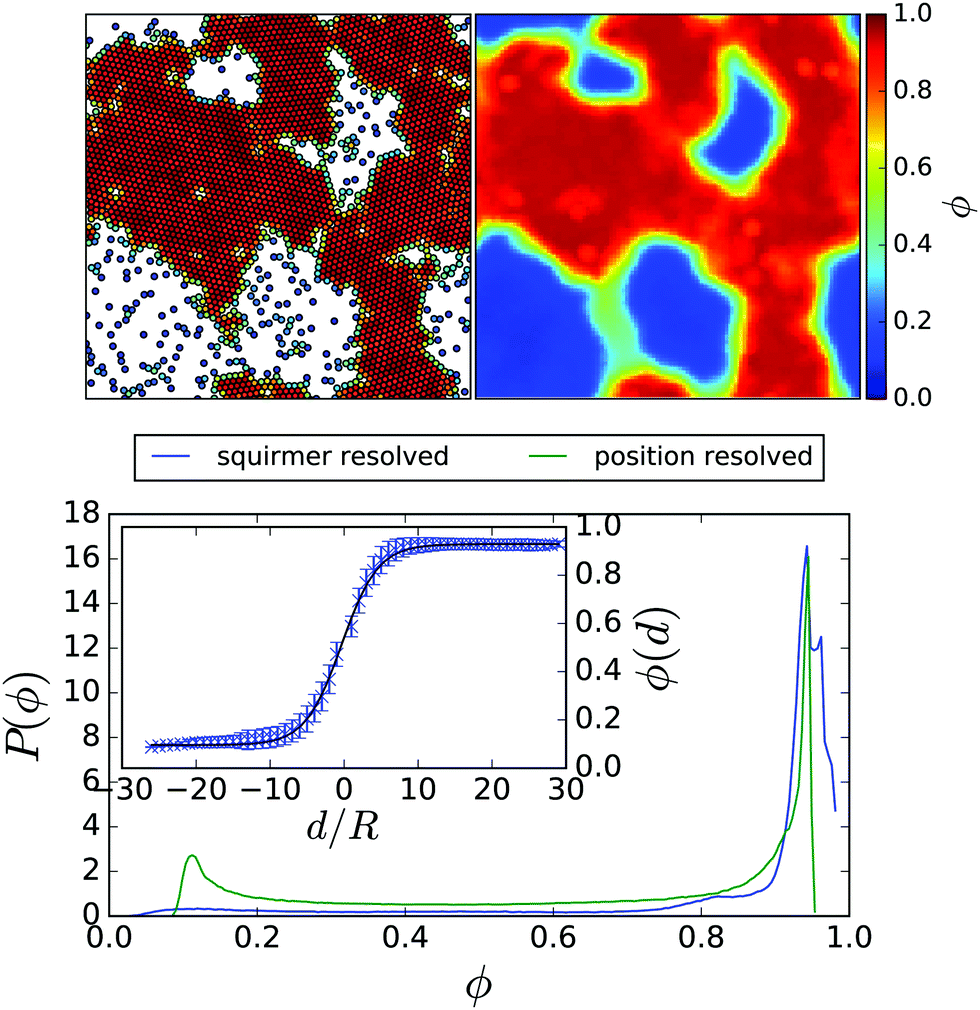 | ||
| Fig. 1 Top, left: Snapshot of squirmer configuration for 3328 squirmers with Pe = 355 (B1 = 0.1) and = 0.64 exhibiting coexistence between a high-density and a low-density phase. The colour code represents the local density ϕi around the i-th squirmer. Top, right: Corresponding position-resolved density ϕ(x,y) averaged over 3 × 10⁶ MPCD time steps. Bottom, main plot: Probability distribution of local density ϕi (blue line). For comparison, the probability of the position-resolved density ϕ(x,y) is shown (green line). Inset: Local density ϕ(d) as a function of distance from an interface, d, measured in units of R. The solid black line is a fit to the interfacial density predicted by Cahn–Hilliard theory. | ||
To quantify the local density, we construct around each squirmer a Voronoi cell and determine its area Ai. The local density within this Voronoi cell is therefore ϕi = 1/Ai. A standard analysis, such as the one used in ref. 35, would be to determine the probability distribution p(ϕi) of local densities ϕi and to identify the densities of the two coexisting phases from the expected bimodal distribution. The probability distribution corresponding to the squirmer snapshot in Fig. 1 is shown in Fig. 1: bottom by the blue line. The dense phase produces a very pronounced peak with a very broad tail, which obscures the signature of the gas phase. This broad tail is due to encounters between a small number of swimmers in the gas phase forming small temporary clusters. Thus, some form of temporal averaging is needed, in order to keep only those dense regions that remain intact and relatively fixed in place.
Hence we divide the system area into a grid with cell spacing equal to the squirmer radius R. Each cell is assigned a local density using a weighted average of the local densities from those Voronoi cells, which intersect each grid cell. We then average over time, choosing the averaging interval to be longer than the life time of temporary clusters, yet short enough so that permanent clusters seem relatively unchanged. Hence, we arrive at a position-resolved density ϕ(x,y) such as the one plotted in Fig. 1: top, right. A histogram of the values of ϕ(x,y) is plotted in Fig. 1: bottom, green line, and recovers the peak for the gas phase.
The color-coded density ϕ(x,y) in Fig. 1 also shows a pronounced interfacial region between dense and gas phase. In order to obtain their densities and distinguish them from the interface, we determine the interfacial density profile ϕ(d), where |d| is the distance to the nearest point on the interface. A preliminary position of the interface is determined by requiring that the time-averaged number of neighbours is three. Variations in this choice simply shift the density profile along the d-axis, but do not alter its shape. Thus the resulting ϕ(d) is independent of fixing the exact interface position beforehand. For each grid cell the distance to each point of the estimated interface is determined and the minimal value is chosen as |d|. Collecting the statistics for each grid cell then gives ϕ(d). The resulting profile corresponding to the color-coded density ϕ(x,y) can be seen in the inset of Fig. 1: bottom. Inspired by ref. 10 and Cahn–Hilliard theory,13 we fit
 | (5) |
Before we introduce the resulting phase diagram, we discuss the coarsening dynamics from the uniform initial state to the final phase-separated system. Fig. 2: top illustrates the time evolution for a system with = 0.48 and Pe = 355 (B1 = 0.1) on different time scales. Initially (first row) clusters of squirmers develop in the unstable uniform phase characteristic for spinodal decomposition. They grow and become denser until a few clusters remain (second row). These clusters already have the final density ϕden of the dense phase. They show the typical coarsening dynamics of a phase-separating system due to diffusive exchange of squirmers between the clusters. Ultimately, one single cluster remains (third row), the shape of which becomes more compact over the course of time.
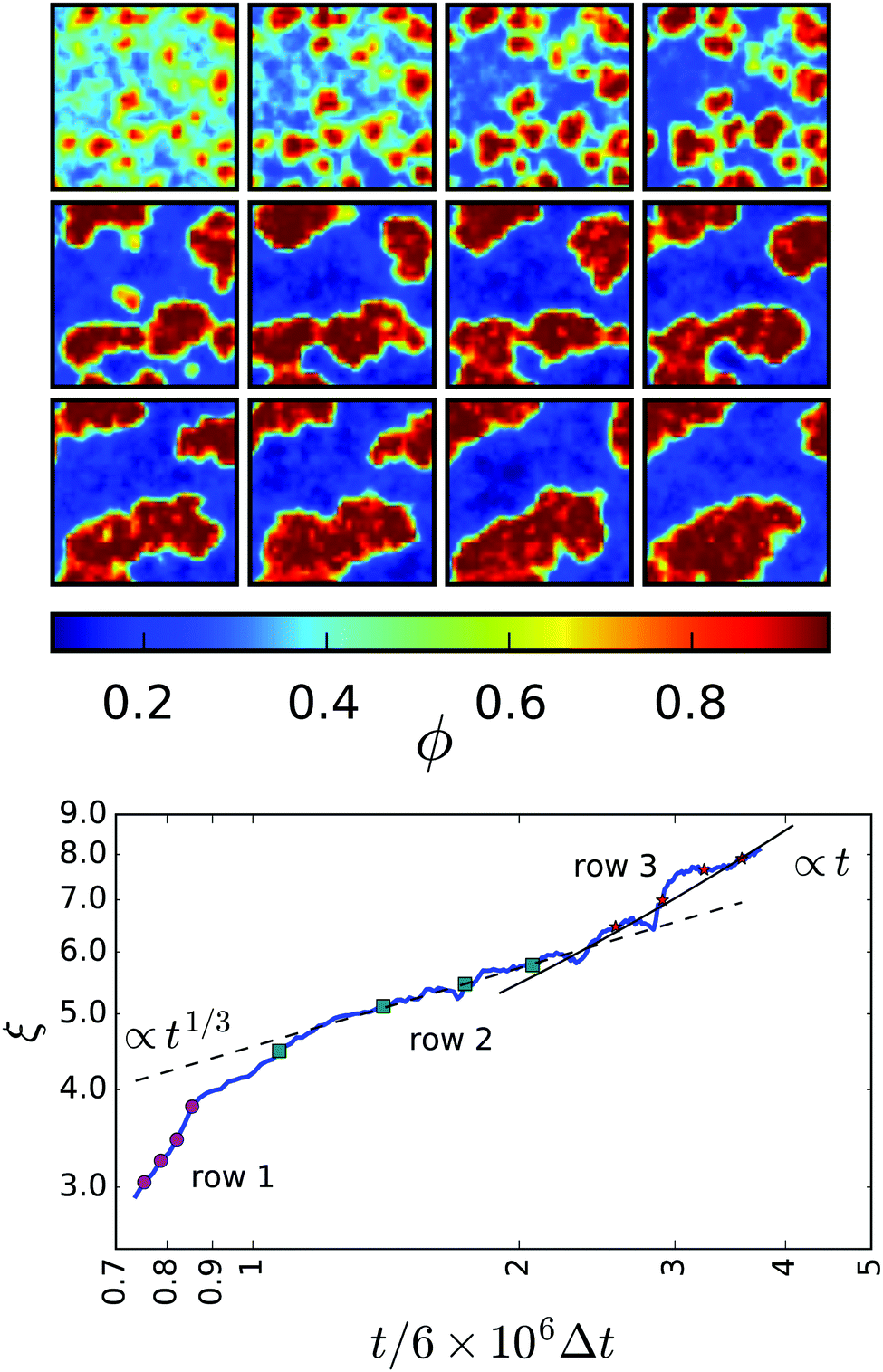 | ||
| Fig. 2 Top: Time evolution of ϕ(x,y). Each successive frame represents a time marked on the plot of ξ(t) (bottom panel). The first, second, and third row are marked by magenta circles, green squares, and red stars, respectively. Bottom: Characteristic cluster size ξ(t) as a function of time (in units of MPCD time step Δt). Simulation data for = 0.48 is shown in the blue solid line. The coarsening dynamics of model H for diffusive transport, ξ(t) ∼ t1/3, and viscous hydrodynamic transport, ξ(t) ∼ t, are indicated by the dashed and solid black lines, respectively. | ||
Following ref. 52, we quantify coarsening by determining the area a(t) of all dense regions and their total perimeter l(t) as a function of time. The mean domain size then becomes ξ(t) := a(t)/l(t). Fig. 2: bottom compares ξ(t) to the different regimes of the coarsening dynamics for a system with conserved order parameter including hydrodynamics.52 After the initial formation of the clusters (the magenta dots refer to the frames in the first row), the total area a(t) remains constant and all further changes in ξ are due to changes in l(t) alone. In the intermediate regime, the mean domain size roughly obeys the scaling expected when diffusive transport dominates, ξ ∼ t1/3 (frames in the second row). This regime lasts less than a decade, since our system size is relatively small. Former work on the coarsening dynamics of pure active Brownian particles report a deviation from the scaling exponent 1/3, measuring 0.25535 or 0.28.53 However, our system is too small to make a clear statement about the exponent. Finally, the compactification of the single cluster gives rise to clearly visible, jumplike increases of ξ(t). For comparison, we give the expected scaling ξ ∼ t due to viscous hydrodynamic transport. This compactification has not been seen for pure active Brownian particles. Also, in our simulations not all enter this regime. Small clusters leave the diffusive transport regime with fairly circular clusters already. Whereas for ≥ 0.50 clusters spanning the whole simulation box are formed. These are stable, either as “slabs” for ≈ 0.50 or the gas phase forms a “bubble” at even larger mean densities. The rapid increase of ξ(t), shown in Fig. 2: bottom towards the end, therefore requires ≲ 0.50 and probably is a finite size effect.
3.2 Phase diagram of neutral squirmers
In Fig. 3: top we plot the densities ϕgas and ϕden of the coexisting gas and dense phases in a Pe–ϕ diagram, which we determined for different mean densities. Interestingly, the resulting binodal lines do not agree. In particular, the gas binodal is shifted to smaller values ϕgas for increasing . In contrast, for pure active Brownian particles, the densities of the two coexisting phases are independent of .11,35 For our geometry we present them in Appendix 5.2. Thus, we suspect hydrodynamic interactions between the squirmers to cause this behaviour. For constant Péclet number Fig. 4 demonstrates how the gas density ϕgas decreases for larger . Thus, the cluster of dense phase, which grows in size with increasing , extracts additional squirmers from the gas phase. Below we will attribute this behaviour to an additional hydrodynamic pressure caused by the squirmers at the interface between the dense and the dilute phase.
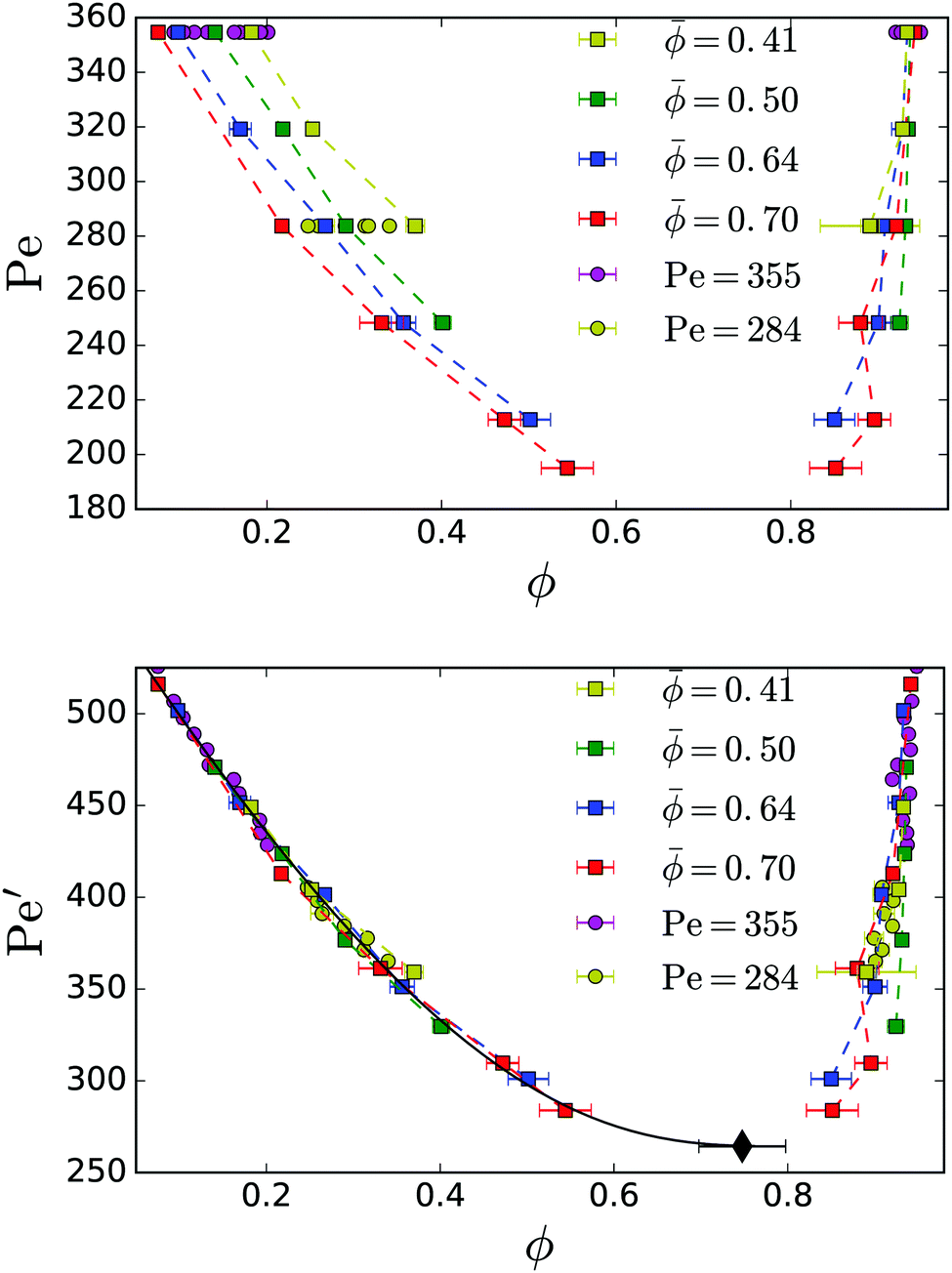 | ||
| Fig. 3 Top: Binodal lines showing the coexistence densities of neutral squirmers for different mean densities . The magenta points for Pe = 355 correspond to simulations from Fig. 4. Bottom: The rescaled data using the effective Péclet number Pe′ = (1 + 0.65) Pe shows a data collapse for different . The black line shows a fit to eqn (7). The fitted critical point is marked by the back diamond. | ||
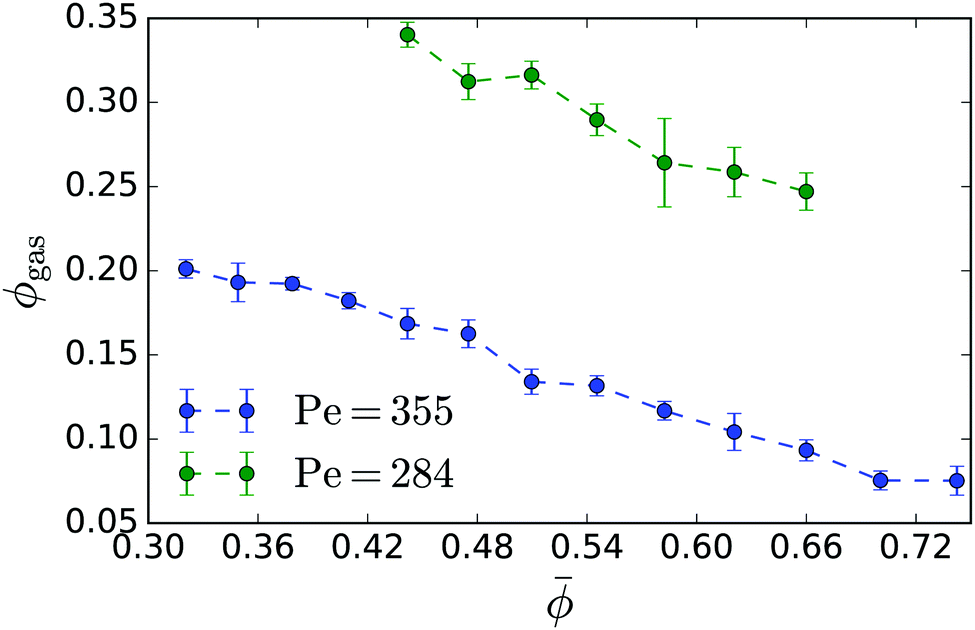 | ||
| Fig. 4 Gas density ϕgas in the phase-separated system plotted versus mean density for neutral squirmers with Pe = 355 (B1 = 0.1) and Pe = 284 (B1 = 0.08). | ||
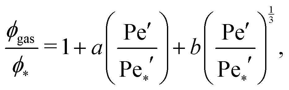
The gas binodals in Fig. 3: top roughly run parallel to each other. Thus, by introducing an effective Péclet number
| Pe′ = (1 + a)Pe | (6) |
) = DT,2D( = 0)/(1 + 2.027) in the definition (4) of the Péclet number. We determined it from the velocity-auto-correlation function and the Green–Kubo formula (see also paragraph after eqn (8) and Appendix 5.3). However, the prediction of 2.027 for the coefficient a cannot explain the reported data collapse.
In order to estimate the position of the critical point (ϕ*,Pe*′), we fit11
 | (7) |
For a system in mechanical equilibrium the total pressure in the coexisting gas and dense phases has to be the same. We now apply this strategy to our system of phase-separating squirmers in order to understand why the binodals depend on the mean density. For active Brownian particles without any hydrodynamic interactions, the pressure balance was first proposed in ref. 9 by introducing a total pressure consisting of a steric and an active contribution: p = p(s) + p(a). This pressure balance was then used in the context of phase separation in ref. 9, 10, 16 and 54–56. The steric pressure results from direct interactions between the squirmers, 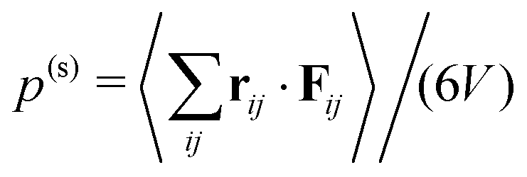 .57 Here, rij = ri − rj is the distance vector from swimmer j to swimmer i, Fij the force with which squirmer j acts on i, V is the volume of a uniform system, and 〈⋯〉 means temporal average. Swimmers moving with constant velocity v0 along the unit vector êi also generate a swim pressure:9
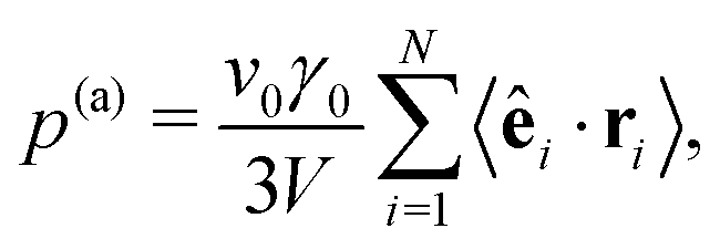 | (8) |
Due to hydrodynamic interactions with bounding walls and other squirmers, the friction coefficient in eqn (8) depends not only on the squirmer's position but also the position of every other squirmer. Hence, it is not possible to know γ0 precisely. To arrive at a sort of mean-field approximation for γ0(ϕ), we use the Green–Kubo formula and determine a self-diffusion coefficient DT,2D(ϕ) from the velocity-auto-correlation function of a passive particle with radius R using the velocity components in the plane of the quasi-two-dimensional geometry. The result is plotted in Fig. 11 of Appendix 5.3 and can be well approximated by DT,2D(ϕ) = DT,2D(ϕ = 0)/(1 + 2.027ϕ). We then use the Einstein relation, γ0(ϕ) = kBT/DT,2D(ϕ), to arrive at a density-dependent friction coefficient. However, the following results only change little compared to working with a constant γ0 = kBT/DT,2D(ϕ = 0) for all densities.
In a dilute gas of non-interacting Brownian particles, orientation decorrelates exponentially on the decorrelation time 2τr and one obtains from eqn (8)9
| p(a)id = ρgasτrγ0v02/6 ∼ ρgasPe2, | (9) |
We are able to calculate steric and the swim pressure of eqn (8) for the local neighbourhood of each squirmer (see Appendix in Section 5 for details). Fig. 5: top shows these local pressure values as a function of the distance from the gas-cluster interface. In light of the discussion about the swim pressure following eqn (8), its pressure values close to the interface have to be treated with caution. But they are not important for the following. Outside the dense phase, d < 0, the steric pressure is low due to very few contacts between squirmers or a squirmer and a bounding wall. And when they do occur, they persist for only a short time. On the other hand, the local swim pressure in the gas phase is large as swimmers can move unhindered. Inside the cluster, d > 0, squirmers are in constant contact with their neighbours and the confining walls. This leads to a significantly higher steric pressure. On the other hand, the squirmer's swimming motion is hindered by the neighbours. Swimming motion and actual displacement are much less correlated and the swim pressure is greatly reduced.
 | ||
| Fig. 5 Top: Local pressure values plotted across the interface between gas and dense phase for Pe = 355 (B1 = 0.1) and = 0.51. Distance from the interface d is measured in units of squirmer radius R. d > 0 represents the interior of the cluster formed by the dense phase. Bottom: Total pressure jump Δ(p(s) + p(a)) when going into the dense phase plotted versus . The black line shows the fit Δp() = 5.1 − 0.95. | ||
However, contrary to what is expected for mechanical equilibrium, the total pressure p = p(s) + p(a) plotted in Fig. 5: top is not the same for the gas and the dense phase. Furthermore, in Fig. 5: bottom we see that this total pressure difference Δp = pden − pgas across the phase interface increases with increasing . Thus, there must be an additional negative pressure stabilizing this interface. When introducing the swim pressure, the authors of ref. 9 already remarked that for swimmers swimming in a fluid environment, the hydrodynamic stresslet induces an additional hydrodynamic pressure. In the following we elaborate on this idea for our special geometry and demonstrate that indeed we are able to justify a negative pressure difference between the dense and the gas phase.
It is not possible to give a complete quantitative theory for the negative hydrodynamic pressure produced by the dense cluster of squirmers. Instead, we present here an approximate treatment, which contains the essential ideas. A squirmer at position r0 and confined between two plates generates the flow field of a source dipole with the approximate dipole moment σ = 2πR2v0ê.40,59 It is accompanied by the pressure field
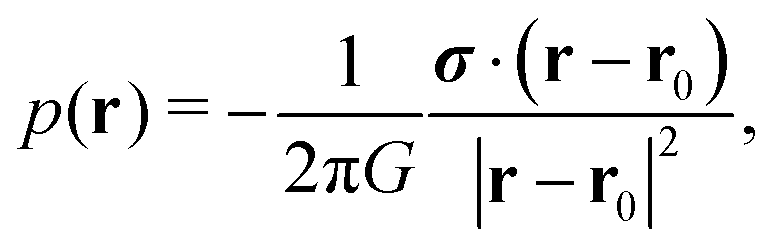 | (10) |
Now, we consider a circular cluster of squirmers and replace the dipole moment σ by a density of source dipoles. Furthermore, we find that on average the squirmers have a tendency to point radially inwards towards the center, especially at the rim of a cluster. Therefore, we introduce a source dipole density ![[small sigma, Greek, macron]](https://www.rsc.org/images/entities/b_i_char_e0d2.gif) = 〈σ·c〉c, where c is a unit vector pointing from the squirmer to the cluster center. The radial dipole density 〈σ·c〉 across the interface from the gas to the dense phase is plotted in Fig. 6 for different . This confirms the preferred radial alignment at the rim of the dense cluster, whereas in the interior the squirmers point towards the bounding walls, on average, since 〈σ·c〉 is zero. We calculate the pressure generated by the dipole density in two steps. First, we integrate along a circle of radius r0 to obtain pressure per unit length:
= 〈σ·c〉c, where c is a unit vector pointing from the squirmer to the cluster center. The radial dipole density 〈σ·c〉 across the interface from the gas to the dense phase is plotted in Fig. 6 for different . This confirms the preferred radial alignment at the rim of the dense cluster, whereas in the interior the squirmers point towards the bounding walls, on average, since 〈σ·c〉 is zero. We calculate the pressure generated by the dipole density in two steps. First, we integrate along a circle of radius r0 to obtain pressure per unit length:
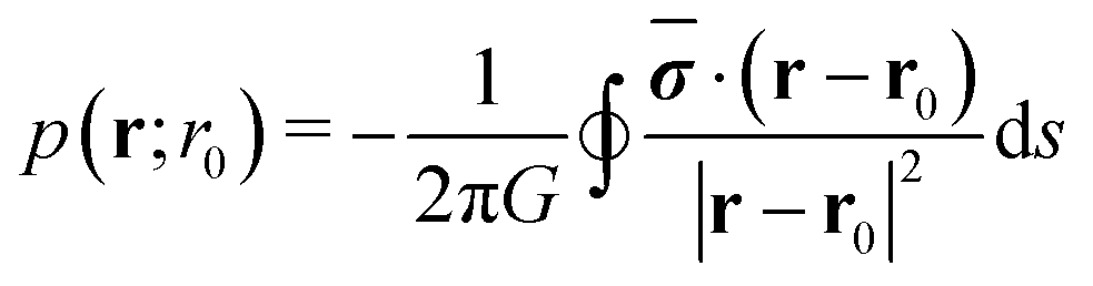 | (11) |
![[thin space (1/6-em)]](https://www.rsc.org/images/entities/char_2009.gif) cosφ, r0sinφ), cosφ = r0·r, and r0 = −r0c one obtains
cosφ, r0sinφ), cosφ = r0·r, and r0 = −r0c one obtains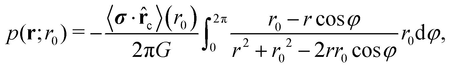 | (12) |
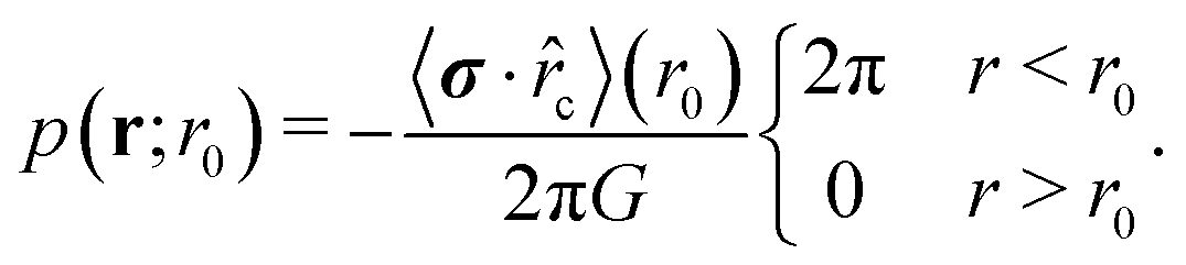 | (13) |
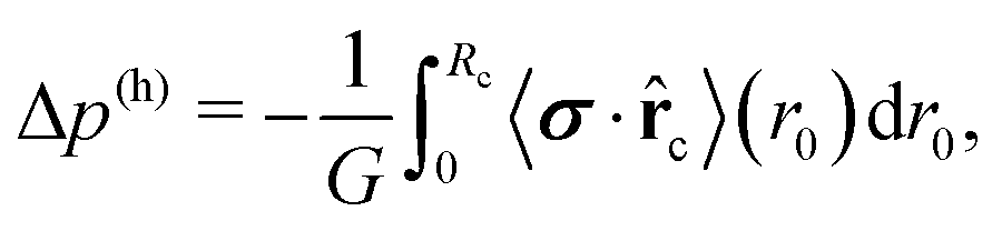 | (14) |
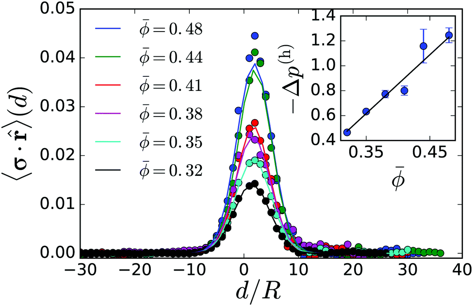 | ||
| Fig. 6 Top: Radial source-dipole density plotted versus distance from the cluster interface, d, measured in units of squirmer radius R for different mean densities . Inset: Magnitude of resulting hydrodynamic pressure difference versus . The solid line shows a fit −Δp(h) = 4.72 − 1.04. | ||
In summary, our argument is as follows: any net polar order of swimmers is accompanied by a jump in solvent pressure, a fact that has also been reported by ref. 60. In our case, this is due to the squirmers at the edge of the cluster: the hydrodynamic pressure difference between cluster interior and exterior is necessary to stop the flow initiated by the squirmers, which try to pump fluid out of the cluster interior.
The inset in Fig. 6 shows the hydrodynamic pressure using the radial source-dipole density 〈σ·c〉 from the main plot. Its absolute value increases linearly with cluster size or , which results from the stronger radial alignment as the cluster size increases. The linear increase of |Δp(h)| coincides with the linear increase of Δ(p(s) + p(a)) plotted in Fig. 5: bottom, however the slope is by a factor of 1.1 too low. This is understandable since we approximate the squirmers in the dense cluster by point-like source dipoles with an approximate dipole moment. We only calculated Δp(h) up to = 0.48, where the dense clusters are nearly circular. Beyond this mean density, they become elongated and the radial alignment of the squirmers cannot clearly be defined.
Thus our claim is that by introducing the negative hydrodynamic pressure generated by squirmes swimming into the cluster at its rim, we are able to maintain mechanical equilibrium. Namely, by defining the total pressure p = p(s) + p(a) + p(h) with the hydrodynamic pressure included, this total pressure should be constant across the interface of gas and dense phase. Our observation that |Δp(h)| increases with cluster size and thus with , explains the different binodals in Fig. 5 and why we can collapse all of them on a single master curve with the help of the effective Péclet number from eqn (6). For an increased |Δp(h)|, a lower Δp(a) ∝ ϕgas is required to maintain the interface and thus ϕgas is reduced.
For phase-separating systems, interface curvature leads to a Laplace pressure and can result in a shift of the coexistence densities.61 We point out that this effect cannot be responsible for the shifted binodals as well as the pressure jump in Fig. 5: bottom. First, the Laplace pressure changes signs as one goes from a droplet to a bubble configuration. In particular, the pressure jump in Fig. 5: top was determined for the “slab” configuration with nearly straight interfaces, where the Laplace pressure should vanish. Second, the coexistence densities of the dilute and dense phase in the middle row of Fig. 2: top do not change while coarsening. However, if Laplace pressure were important in our system, the densities would change since the curvature of the interfaces changes.
Until now we have only examined neutral squirmers. In the following we present binodal lines for different squirmer parameter β to demonstrate how pushers and pullers effect the phase-coexistence region of microswimmers.
3.3 Binodal lines of pushers and pullers
The flow field around squirmers is strongly controlled by the dipole strength β used in our swimmer model. For β ≠ 0, the flow field of a single squirmer in a bulk fluid is reminiscent of pushers (β < 0) and pullers (β > 0).1,62 It has a strong effect on how swimmers reorient due to nearby surfaces or other squirmers as demonstrated in ref. 1, 28 and 62. The qualitative effect of increasing |β| has been shown in our earlier work28 to largely suppress phase separation, requiring systems of increasing in order for stable clusters to form.
The binodal lines for different β are compared to the neutral-swimmer case in Fig. 7 for pushers (top panel) and pullers (bottom panel). The overall trend is that for increasing |β| the coexistence regime becomes smaller. For pushers, one realizes very nicely how the binodals are mainly shifted up, thereby increasing the critical Péclet number. The same applies to pullers, however, the gas binodals are also deformed compared to β = 0. We observe that puller squirmers are more mobile in the dense phase compared to pushers. Therefore, the corresponding binodals are shifted to smaller ϕ.
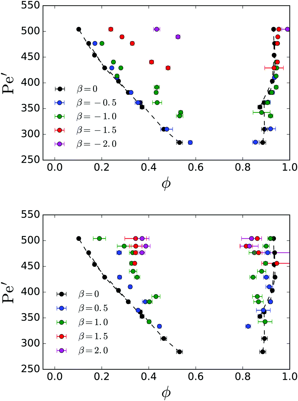 | ||
| Fig. 7 Binodal lines of pushers (top panel) and pullers (bottom panel) for different dipole strengths β. For reference, the data from Fig. 3: bottom is shown as black. | ||
For pushers and pullers in full three dimensions spontaneous polar order was observed for small but non-zero β.39 This results in a net motion of swimmers along a common direction. We do not find such a net motion for small β in our simulations. This might be due to the fact that in our quasi-two-dimensional geometry the far fields of neutral and non-neutral squirmers both decay as 1/r2.40,59 Thus, squirmers with small β ≠ 0 do not have a sufficiently different far field compared to neutral squirmers.
3.4 Melting of the cluster phase
In the region below the critical Péclet number in Fig. 3: bottom the phase is isotropic. On the other hand, at large effective Péclet numbers we observe hexagonal order in the dense phase, which hence has to undergo a melting transition if the Péclet number is reduced. It is not our intention to present a thorough discussion of this subtle phenomenon but to only give an indication for melting.The dense branch of the binodal lines of neutral squirmers and of pushers (see Fig. 7: top) reveal a similar trend. At Pe′ ≈ 400 and below, the density of the dense phase decreases and stabilizes at a lower value around Pe′ ≈ 350. In particular, this feature is clearly seen for neutral squirmers and coincides with a loss of hexagonal order in the cluster. As in ref. 28 we introduce the bond parameter |q6|2 to measure local sixfold bond-orientational order around a squirmer. In Fig. 8 we plot the probability distribution for |q6|2 in the dense phase for a range of Pe′. For Pe′ ≥ 402 a peak at |q6|2 ≈ 1 dominates the distribution and indicates hexagonal order in the dense phase. The hexagonal domains are stable over time with only short perturbations when defects and vacancies move through the hexagonal lattice due to the random component of the squirmers' motions. These perturbations slightly reduce the time-averaged |q6|2 and shift the peak position below 1.
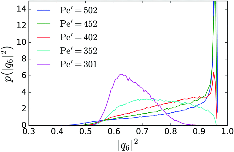 | ||
| Fig. 8 Probability distribution of the six-fold bond parameter |q6|2 within the cluster phase for = 0.64 and a range of effective Péclet numbers Pe′. | ||
Below Pe′ ≥ 402 the sharp peak in the distribution function disappears indicating a melting transition with a loss of hexagonal order. In the simulations we still observe stable clusters, which now form fluid droplets. During the melting transition we also observe an increase of the mobility of the squirmers by a factor of 5–10, when monitoring the mean-square displacement in the dense phase. The ESI† contains Videos M5 and M6 showing the hexagonal and fluid dense phase, respectively. In Video M6 (ESI†) we see that, although hexagonal patches exist, they are not stable over time. Finally, when lowering Pe′ towards the critical point, the fluid cluster “evaporates” as the system exits the phase-coexistence regime.
4 Summary and conclusion
We have studied the phase separation of model hydrodynamic microswimmers called squirmers in quasi-two-dimensional confinement extending our previous investigations.28 The full three-dimensional hydrodynamics was simulated in order to accurately capture the squirmer interactions. This makes our simulations a realistic representation of real-world artificial and biological microswimmers. By employing a parallelized implementation of the MPCD algorithm on over 1008 CPU cores, we were able to simulate thousands of squirmers, allowing us to quantitatively determine the binodal lines for different mean densities and squirmer parameters β. The coarsening dynamics towards the phase-separated system shows a characteristic intermediate diffusive regime and a final rather ballistic regime due to compactification of the dense squirmer cluster. However, most strikingly, we found that the position of the binodal lines is strongly influenced by . This effect has not been observed for active Brownian particles, which only interact sterically, and thus is of real hydrodynamic origin. We were able to collapse the different binodals on a single master curve by introducing an effective Péclet number. Extending the mechanical pressure balance of ref. 9 and 10 by a hydrodynamic pressure due to the squirmer flow field, the reason for the different binodals became apparent.
We also explored the dependence of the binodal line on β, a parameter which allows us to tune the swimmer type and their flow fields between pushers and pullers. We found that in all cases going to strong pushers or pullers suppresses phase separation by shifting the phase-coexistence region to larger Péclet numbers. The shape of the coexistence region does, however, depend on whether the squirmers are pushers or pullers.
Finally, we examined the structure of the dense phase as the squirmers' swimming speed, the Péclet number, is reduced. We find that fast squirmers in the dense phase form a hexagonal cluster, which melts with decreasing Péclet number into a fluid cluster. This is expected since close to the critical Péclet number the swimmer fluid is isotropic.
5 Appendix
5.1 Position-resolved time averaging
In order to associate an average quantity to a position, one commonly divides up the system into a grid. We call each cell of the grid a “pixel”. A spatially-resolved average can thus be found by simply averaging over the squirmers in each pixel. Since we have only a few thousand squirmers, each pixel would need to be relatively large in order to capture enough squirmers per pixel. This would prevent the accurate resolution of the phase interface.We will use the local density to illustrate our method. First we partition the system into its Voronoi cells. Each Voronoi cell contains a single squirmer, and thus its local density is ϕi = 1/Ai where Ai is the area of the i-th Voronoi cell. Our grid of pixels is then assigned a local density
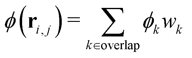 | (15) |
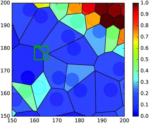 | ||
| Fig. 9 Illustration for the spatially-resolved time average of local density. Each Voronoi cell with area Ai is assigned a local density ϕi = 1/Ai (colorbar). The average density at a pixel (green square) is the weighted average of the local density in all overlapping Voronoi cells, based on the degree of overlap. | ||
All time averages are taken with respect to a specific spatial position. Due to the motion of the squirmers, the time averages of ϕ(ri,j) eventually wash out the structure of the Voronoi construction, leaving only those density inhomogeneities that are stationary in space. We use the same construction for calculating local pressure and |q6|2 values.
5.2 Comparison with active brownian particles
Fig. 10 compares the binodals from Fig. 3 with those for active Brownian particles in quasi two dimensions. Brownian dynamics simulations where conducted for the same range of parameters and the same geometry as the full hydrodynamic simulations. Similarly to simulations conducted in two dimensions11 for the range of Péclet numbers simulated, the coexistence densities for active Brownian particles did not vary much. We also note that the binodals for two different mean densities = 0.41 and = 0.70 lie on top of each other. For comparison, the binodals for the hydrodynamically interacting (HI) squirmers from Fig. 3 are shown.
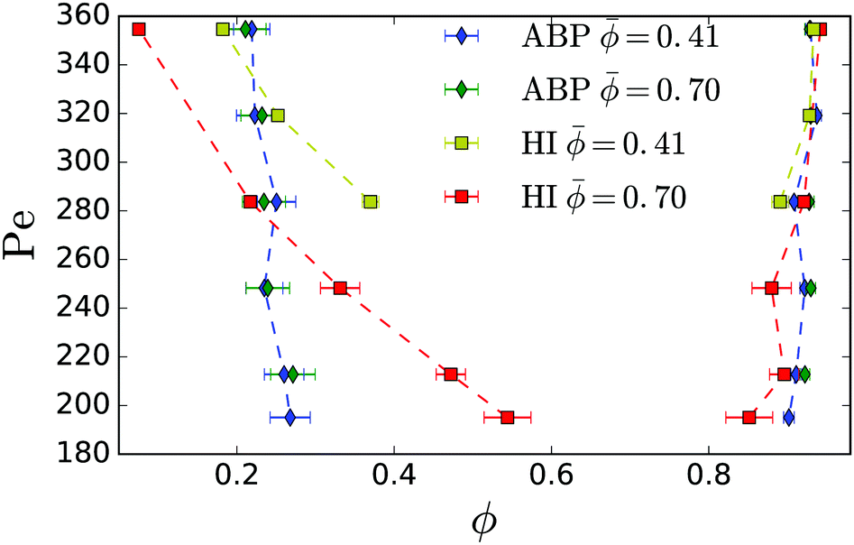 | ||
| Fig. 10 Comparison between binodals for active Brownian particles (ABP) and the binodals for squirmers (HI) from Fig. 3. Mean densities and Péclet numbers, as well as simulation box size and squirmer radius correspond to the range used for the full hydrodynamic simulations. | ||
5.3 Position-resolved swim and steric pressure
Before we explain, how we calculate the pressure values, we present in the inset of Fig. 11 the velocity-auto-correlation function for the in-plane velocity components of a passive particle, determined in MPCD simulations for different mean densities of passive particles. The self-diffusion coefficient is then plotted in the main graph of Fig. 11 and fitted by DT,2D(ϕ) = DT,2D(ϕ = 0)/(1 + 2.027ϕ). Using the Einstein relation, we obtain a density-dependent friction coefficient, γ0(ϕ) = kBT/DT,2D(ϕ).
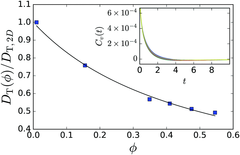 | ||
| Fig. 11 Self-diffusion coefficient of passive particles plotted versus their density ϕ confined between two walls with distance H = 8R/3. The full line is a fit to DT,2D(ϕ) = DT,2D(ϕ = 0)/(1 + bϕ) with b = 2.027. Inset: The corresponding in-plane velocity-auto-correlation functions Cv(t) = 〈v(t)·v(0)〉/2kBT for the different densities in the main plot. The differences are rather subtle. Time is given in MPCD units. | ||
Now, we apply eqn (8) to the individual Voronoi cells and its surround neighbours (cf.Fig. 12). Our system volume now is Vi ≈ HAi, i.e., the height of the system H times the 2D-Voronoi cell area Ai, and the neighbours are the immediate neighbours in terms of the Voronoi cell. On this level, the force generating the active motion Fswim = γ0vj of neighbouring squirmers will act on the central Voronoi cell, i.e. inducing a pressure on its “walls”. There is an additional subtlety here: the position vectors rj of the neighboring squirmers always have to start from the central swimmer, for which local pressure is calculated, otherwise shear terms would appear in the derivation of eqn (8).63 Furthermore, the mean velocity also needs to be subtracted from the individual swimmer velocities. Thus we are performing calculations in the centre-of-mass frame of the neighbourhood of each squirmer. We reduce the amount of fluctuations by taking the time average for each pixel (cf. previous subsection on spatial averaging). This time average is longer than the decorrelation time DR−1 of the swimmers as required by eqn (8).
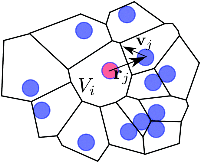 | ||
Fig. 12 Illustration of the swim pressure in the central Voronoi cell (central particle colored in red). The coordinate system is centred at the central particle. Its Voronoi cell has a volume Vi. Nearby particles exert a swim pressure  “on” the Voronoi cell of the central particle, where j runs over all neighboring Voronoi cells. “on” the Voronoi cell of the central particle, where j runs over all neighboring Voronoi cells. | ||
Similarly, we use the Voronoi cells to also introduce a local steric pressure following ref. 57. The steric forces acting on one squirmer include forces from its neighbors and also from the bounding walls.
Acknowledgements
We would like to thank I. Aranson, R. Golestanian, G. Gompper, R. Kapral, K. Kroy, T. Speck, and J. Tailleur for stimulating discussions and the referees for their very helpful feedback. This project was funded under the DFG priority program SPP 1726 “Microswimmers – from Single Particle Motion to Collective Behaviour” (grant number STA352/11). Simulations were conducted at the “Norddeutscher Verbund für Hoch- und Höchstleistungsrechnen” (HLRN), project number bep00050.References
- A. Zöttl and H. Stark, J. Phys.: Condens. Matter, 2016, 28, 253001 CrossRef.
- S. Herminghaus, C. C. Maass, C. Krüger, S. Thutupalli, L. Goehring and C. Bahr, Soft Matter, 2014, 10, 7008–7022 RSC.
- M. C. Marchetti, J. F. Joanny, S. Ramaswamy, T. B. Liverpool, J. Prost, M. Rao and R. A. Simha, Rev. Mod. Phys., 2013, 85, 1143–1189 CrossRef CAS.
- D. Saintillan and M. J. Shelley, C. R. Phys., 2013, 14, 497–517 CrossRef CAS.
- I. S. Aranson, C. R. Phys., 2013, 14, 518–527 CrossRef CAS.
- R. Kapral, J. Chem. Phys., 2013, 138, 020901 CrossRef PubMed.
- J. Palacci, S. Sacanna, A. P. Steinberg, D. J. Pine and P. M. Chaikin, Science, 2013, 339, 936–940 CrossRef CAS PubMed.
- I. Theurkauff, C. Cottin-Bizonne, J. Palacci, C. Ybert and L. Bocquet, Phys. Rev. Lett., 2012, 108, 268303 CrossRef CAS PubMed.
- S. C. Takatori, W. Yan and J. F. Brady, Phys. Rev. Lett., 2014, 113, 028103 CrossRef CAS PubMed.
- J. Bialké, J. T. Siebert, H. Löwen and T. Speck, Phys. Rev. Lett., 2015, 115, 098301 CrossRef.
- T. Speck, A. M. Menzel, J. Bialké and H. Löwen, J. Chem. Phys., 2015, 142, 224109 CrossRef PubMed.
- K. Schaar, A. Zöttl and H. Stark, Phys. Rev. Lett., 2015, 115, 038101 CrossRef PubMed.
- R. Wittkowski, A. Tiribocchi, J. Stenhammar, R. J. Allen, D. Marenduzzo and M. E. Cates, Nat. Commun., 2014, 5, 4351 CAS.
- M. E. Cates and J. Tailleur, Annu. Rev. Condens. Matter Phys., 2015, 6, 219–244 CrossRef CAS.
- J. Stenhammar, R. Wittkowski, D. Marenduzzo and M. E. Cates, Phys. Rev. Lett., 2015, 114, 018301 CrossRef PubMed.
- A. P. Solon, J. Stenhammar, R. Wittkowski, M. Kardar, Y. Kafri, M. E. Cates and J. Tailleur, Phys. Rev. Lett., 2015, 114, 198301 CrossRef PubMed.
- T. Speck, J. Bialké, A. M. Menzel and H. Löwen, Phys. Rev. Lett., 2014, 112, 218304 CrossRef.
- J. Bialké, H. Löwen and T. Speck, EPL, 2013, 103, 30008 CrossRef.
- J. Tailleur and M. E. Cates, Phys. Rev. Lett., 2008, 100, 218103 CrossRef CAS PubMed.
- K. Drescher, K. C. Leptos, I. Tuval, T. Ishikawa, T. J. Pedley and R. E. Goldstein, Phys. Rev. Lett., 2009, 102, 168101 CrossRef PubMed.
- J. Simmchen, J. Katuri, W. E. Uspal, M. N. Popescu, M. Tasinkevych and S. Sánchez, Nat. Commun., 2015, 7, 10598 CrossRef PubMed.
- I. Buttinoni, J. Bialké, F. Kümmel, H. Löwen, C. Bechinger and T. Speck, Phys. Rev. Lett., 2013, 110, 238301 CrossRef PubMed.
- J. Palacci, C. Cottin-Bizonne, C. Ybert and L. Bocquet, Phys. Rev. Lett., 2010, 105, 088304 CrossRef PubMed.
- S. Thutupalli, R. Seemann and S. Herminghaus, New J. Phys., 2011, 13, 073021 CrossRef.
- M. Schmitt and H. Stark, EPL, 2013, 101, 44008 CrossRef.
- C. C. Maass, C. Krüger, S. Herminghaus and C. Bahr, Annu. Rev. Condens. Matter Phys., 2016, 7, 171–193 CrossRef CAS.
- M. Schmitt and H. Stark, Eur. Phys. J. E: Soft Matter Biol. Phys., 2016, 39, 80 CrossRef CAS PubMed.
- A. Zöttl and H. Stark, Phys. Rev. Lett., 2014, 112, 118101 CrossRef PubMed.
- E. M. Purcell, Am. J. Phys., 1977, 45, 3 CrossRef.
- M. J. Lighthill, Commun. Pure Appl. Math., 1952, 5, 109–118 CrossRef.
- J. R. Blake, J. Fluid Mech., 1971, 46, 199–208 CrossRef.
- H. A. Stone and A. D. T. Samuel, Phys. Rev. Lett., 1996, 77, 4102–4104 CrossRef CAS PubMed.
- T. Ishikawa, M. P. Simmonds and T. J. Pedley, J. Fluid Mech., 2006, 568, 119–142 CrossRef.
- M. T. Downton and H. Stark, J. Phys.: Condens. Matter, 2009, 21, 204101 CrossRef PubMed.
- G. S. Redner, M. F. Hagan and A. Baskaran, Phys. Rev. Lett., 2013, 110, 055701 CrossRef PubMed.
- J. Stenhammar, D. Marenduzzo, R. J. Allen and M. E. Cates, Soft Matter, 2014, 10, 1489–1499 RSC.
- A. Wysocki, R. G. Winkler and G. Gompper, EPL, 2014, 105, 48004 CrossRef.
- X. Yang, M. L. Manning and M. C. Marchetti, Soft Matter, 2014, 10, 6477–6484 RSC.
- F. Alarcon and I. Pagonabarraga, J. Mol. Liq., 2013, 185, 56–61 CrossRef CAS.
- T. Brotto, J.-B. Caussin, E. Lauga and D. Bartolo, Phys. Rev. Lett., 2013, 110, 038101 CrossRef PubMed.
- M. Hennes, K. Wolff and H. Stark, Phys. Rev. Lett., 2014, 112, 238104 CrossRef PubMed.
- G.-J. Li and A. M. Ardekani, Phys. Rev. E: Stat., Nonlinear, Soft Matter Phys., 2014, 90, 013010 CrossRef PubMed.
- N. Oyama, J. J. Molina and R. Yamamoto, Phys. Rev. E, 2016, 93, 043114 CrossRef PubMed.
- C. Krüger, C. Bahr, S. Herminghaus and C. C. Maass, Eur. Phys. J. E: Soft Matter Biol. Phys., 2016, 39, 1–9 CrossRef PubMed.
- H. Noguchi, N. Kikuchi and G. Gompper, EPL, 2007, 78, 10005 CrossRef.
- J. T. Padding and A. A. Louis, Phys. Rev. E: Stat., Nonlinear, Soft Matter Phys., 2006, 74, 031402 CrossRef CAS.
- A. Zöttl and H. Stark, PhD thesis, Technische Universität Berlin, 2014.
- H. Noguchi and G. Gompper, Phys. Rev. E: Stat., Nonlinear, Soft Matter Phys., 2008, 78, 016706 CrossRef PubMed.
- I. Götze, H. Noguchi and G. Gompper, Phys. Rev. E: Stat., Nonlinear, Soft Matter Phys., 2007, 76, 046705 CrossRef PubMed.
- I. O. Götze and G. Gompper, Phys. Rev. E: Stat., Nonlinear, Soft Matter Phys., 2010, 82, 041921 CrossRef PubMed.
- A. Imperio, J. T. Padding and W. Briels, Phys. Rev. E: Stat., Nonlinear, Soft Matter Phys., 2011, 83, 046704 CrossRef CAS PubMed.
- A. J. Bray, Philos. Trans. R. Soc., A, 2003, 361, 781–791 CrossRef CAS PubMed.
- J. Stenhammar, A. Tiribocchi, R. J. Allen, D. Marenduzzo and M. E. Cates, Phys. Rev. Lett., 2013, 111, 145702 CrossRef PubMed.
- A. P. Solon, Y. Fily, A. Baskaran, M. E. Cates, Y. Kafri, M. Kardar and J. Tailleur, Nat. Phys., 2015, 11, 673–678 CrossRef CAS.
- R. G. Winkler, A. Wysocki and G. Gompper, Soft Matter, 2015, 11, 6680–6691 RSC.
- S. C. Takatori and J. F. Brady, Phys. Rev. E: Stat., Nonlinear, Soft Matter Phys., 2015, 91, 032117 CrossRef CAS PubMed.
- D. H. Tsai, J. Chem. Phys., 1979, 70, 1375 CrossRef CAS.
- J. Brady, private communication.
- J. B. Delfau, J. Molina and M. Sano, EPL, 2016, 114, 24001–24006 CrossRef.
- W. Yan and J. F. Brady, Soft Matter, 2015, 11, 6235–6244 RSC.
- A. Statt, P. Virnau and K. Binder, Phys. Rev. Lett., 2015, 114, 026101 CrossRef PubMed.
- S. E. Spagnolie and E. Lauga, J. Fluid Mech., 2012, 700, 105–147 CrossRef.
- T. Speck, EPL, 2016, 114, 30006–30007 CrossRef.
Footnotes |
| † Electronic supplementary information (ESI) available: 6 video files. See DOI: 10.1039/c6sm02042a |
| ‡ One can argue that the linear exention of the volume V should be larger than the persistence length of the swimmer. However, if one averages over a sufficiently long time so that a sufficient number of swimmers enter and leave V, this requirment might be relaxed. This needs to be checked more carefully in a future investigation. |
| This journal is © The Royal Society of Chemistry 2016 |