DOI:
10.1039/C6RA03547G
(Communication)
RSC Adv., 2016,
6, 30199-30204
On the dissolution state of cellulose in aqueous tetrabutylammonium hydroxide solutions
Received
7th February 2016
, Accepted 10th March 2016
First published on 14th March 2016
Abstract
We have characterized the dissolution state of microcrystalline cellulose (MCC) in aqueous 40 wt% tetrabutylammonium hydroxide (TBAH) using a combination of light and small angle X-ray scattering, up to 0.1 g cm−3. In dilute solutions, cellulose–cellulose interactions are repulsive, as seen by a positive second virial coefficient. Above 0.04 g cm−3, interactions shift from repulsive to be effectively attractive and cellulose begin to form aggregates that can be modelled as mass fractal clusters. The small angle X-ray scattering data also indicate that cellulose is preferentially solvated by TBA+ ions. We propose that the apparent shift in effective interactions is due to a phase transition where less soluble cellulose II precipitates while cellulose I still dissolves.
Introduction
Cellulose is the World's most abundant biopolymer and hence an important renewable raw material for many materials, like textile fibers and films.1,2 For such applications, however, it is necessary to first dissolve the cellulose pulp. Dissolving cellulose has turned out to be a challenge.3–5 Cellulose is insoluble in most classical polar and non-polar solvents, but is soluble in certain ionic liquids and also partly in concentrated NaOH. The latter being used in the viscose process, developed in the early 1900's.6 Replacing sodium with the more hydrophobic tetrabutyl ammonium cation, appears to improve cellulose solubility.7–10
For applications of cellulose solutions, detailed knowledge of the dissolution state, interactions and solution structure are useful. Optimum spinning conditions generally require particular rheological properties, which in turn may depend strongly on the dissolution state of the cellulose. The scattering of X-rays and visible light allows for characterizing polymer solution structure and interactions on the colloidal length scale.11 Static light scattering (SLS) is often used to determine polymer molecular weight and overall interactions. Small angle X-ray scattering (SAXS), on the other hand, probes the structure on shorter length scales, carrying information on radius of gyration, coil fractal dimension and persistence length. In this paper we combine SLS and SAXS in the characterization of the dissolution state of cellulose when dissolved in aqueous 40 wt% tetrabutyl ammonium hydroxide, TBAH(aq), the cellulose source being microcrystalline cellulose (MCC).
Materials and methods
Materials
Microcrystalline cellulose was obtained from Sigma-Aldrich (Avicel PH-101) as a white powder, having a z-averaged molar mass of Mz = 57 kg mol−1 as obtained from SEC-MALS.12 Tetrabutylammonium hydroxide (TBAH) was obtained as a 40 wt% aqueous solution from Sigma-Aldrich. Both materials were used as received. The cellulose solutions were prepared by weight and the cellulose powder was added to the solvent followed by vigorous stirring until the powder was dissolved. Samples were prepared in a concentration range from 0.0025–0.1 g cm−3. In the binary TBAH–water system 2 clathrate phases are present.13 Below 26 °C 40 wt% TBAH is in a clathrate-solution two phase region and particular attention has to be given in the handling of the solutions, i.e. melting eventual clathrates before sample preparation. Samples containing cellulose were stored for several days at room temperature without any sign of clathrate formation in wide angle diffraction experiments, nor any viscosity increase. Scattering experiments here were performed at 25 °C and refractometry at ambient temperature (≈22 °C).
Refractometry
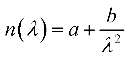
The refractive index, n, and refractive index increment, dn/dc, was determined on a Abbe 60/ED refractometer. The refractive indices were determined at three wavelengths, 435.8, 546.1, and 579.0 nm and at several cellulose concentrations; 0, 0.001, 0.0025, 0.005, 0.0075 and 0.01 g cm−3. The refractive indices were determined at the three wavelengths using the Abbe Utility software. Hereafter, the refractive index was obtained at 632.8 nm using Cauchy's empirical equation  . The refractive index of 40 wt% TBAH(aq) was determined to be 1.406(3) and dn/dc 0.108 cm3 g−1 at ambient temperature.
Static light scattering
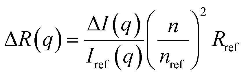
The light scattering study was performed on a goniometer system from ALV Gmbh (Langen, Germany). The instrument of the type ALV/DLS/SLS-5022F has a He–Ne laser with a (in vacuum) wavelength of λ0 = 632.8 nm, a cylindrical quartz vat filled with decaline for refractive-index matching and a detection unit comprises of two matched avalanche photodiodes. The static light scattering (SLS) was performed at scattering angles 30° ≤ θ ≤ 140°, with steps of 10° and an acquisition time of 10 s. The sample was contained in a vial with a path length of 5 mm. Prior to measuring, the samples were centrifuged for 1 hour at 4000 rpm to remove dust. The background subtracted scattering intensity ΔI(q) was converted to absolute scale, i.e. the excess Rayleigh ratio, ΔR(q), according to11| |
 | (1) |
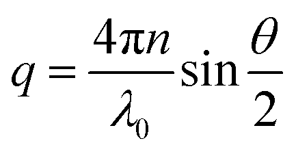
where Iref(q), nref and Rref are the scattered intensity, refractive index and Rayleigh ratio, respectively, of the reference, here being toluene. n is the refractive index of the cellulose solution. q is the scattering vector magnitude, given by| |
 | (2) |
Static light scattering measurements were limited to cellulose concentrations c ≤ 0.01 g cm−3, due to still remaining dust particles after centrifugation. Dust particles occasionally entering the scattering volume gave rise to a high scattered intensity. When this occurred, experiments were repeated. For c > 0.01 g cm−3 dust particles were too frequently present within the scattering volume to allow data correction in this way.
Small-angle X-ray scattering
The small-angle X-ray scattering was performed on an in-house pinhole instrument (Ganesha) from SAXSLAB A/S. The scattering data was collected at two sample-to-detector distances enabling coverage of a total q-range of 0.004–0.7 Å−1. At both sample-to-detector distances a two-pinhole setup whit scatter less slits and a X-ray wavelength of 1.54 Å was used and the scattering patterns were collected on a 300k Pilatus detector. All samples were measured in reusable quartz capillaries at ambient temperature. The entire setup was evacuated. The acquisition time for the 0.02 g cm−3 sample was 8 hours at the shorter sample-to-detector distance and 12 hours at the longer distance. The acquisition times for the following concentrations, 0.03–0.1 g cm−3, were scaled accordingly. All buffers and samples were collected in the same capillary. The azimuthal averaging of the 2D images and background subtractions were performed using the SAXSGUI software. The data was brought to absolute scale using water as a primary standard.
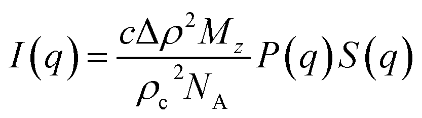
In dilute solutions, the SAXS intensity can be written as11
| |
 | (3) |
here,
c is the cellulose concentration (mass per volume), Δ
ρ = 4.0 × 10
10 cm
−2 is the scattering length density difference between cellulose and solvent,
ρc = 1.5 g cm
−3 is the cellulose density,
Mz is the
z-averaged cellulose molar weight, and
NA is Avogadro's number.
P(
q) and
S(
q) are the form and structure factor, respectively. These are averaged quantities because of the cellulose polydispersity. The cellulose molecules were modelled as semi-flexible chains, as will be further described below. In SAXS,
q is still given by
eqn (2), however with
n = 1.
Results and discussion
Static light scattering
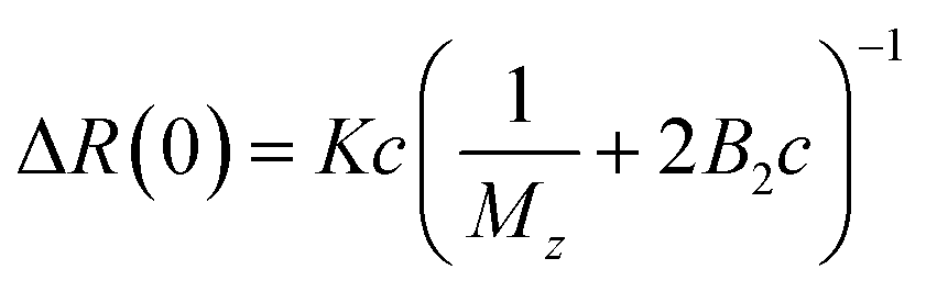
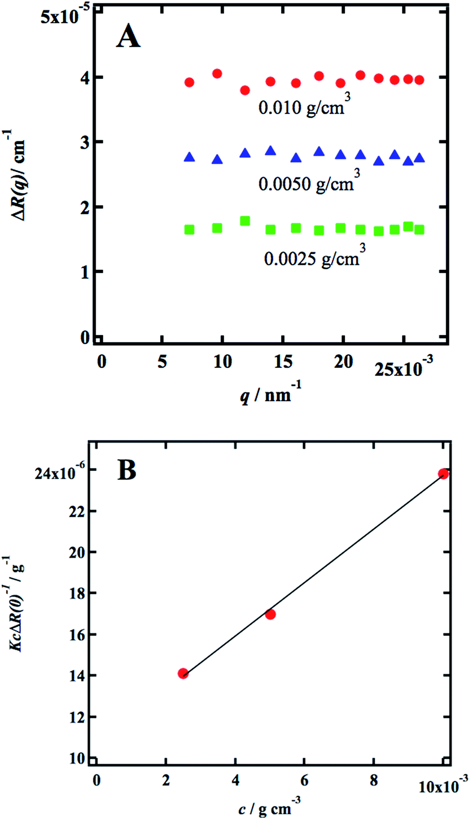
Static light scattering (SLS) experiments were performed on dilute solutions. Three samples were measured, 0.0025, 0.0050, and 0.010 g cm−3, respectively, and in Fig. 1a we present the q-dependence of the absolute scattered intensity ΔR(q). The scattered intensity is essentially q-independent, implying that indicating that the radius of gyration, Rg ≪ 1/qmax ≈ 40 nm, which in turn is a strong indication that the cellulose is fully molecularly dissolved. The SLS data were further analyzed in terms of the excess Rayleigh ratio, ΔR(q), extrapolated to the scattering vector q = 0, which up to the second virial coefficient, B2, often is written as11| |
 | (4) |
where c is the cellulose concentration and Mz is the z-averaged molecular mass. K is the optical constant given by:| |
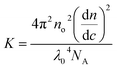 | (5) |
where no = 1.4063 is the refractive index of the solvent, dn/dc = 0.108 cm3 g−1 the refractive index increment, and NA is Avogadro's number. With the laser wave length λ0 = 632.8 nm, we have K = 9.43 × 10⁻⁸ cm2 g−2. In Fig. 1b we have plotted Kc/ΔR(0) as a function of the cellulose concentration, for which eqn (4) predicts a linear relationship with the slope 2B2, and 1/Mz being the intercept. The line in Fig. 1b corresponds to Mz = 93 kg mol−1, and the apparent second virial coefficient, B2 = 6.7 × 10⁻⁴ cm3 g−2. The molecular weight is approximately 60% higher than the value Mz = 57 kg mol−1 obtained from SEC-MALS11 of the same material. The reason for this discrepancy is unclear. We will in the analysis of the SAXS data below use Mz = 93 kg mol−1, the B2 value is slightly positive, although small, indicating repulsive cellulose–cellulose interactions and consistent with 40% TBAH(aq) being close to a θ-solvent for cellulose. For excluded volume interaction we can estimate B2 from14| |
 | (6) |
where Rg is the radius of gyration and M the molecular weight, that both here are number averages. Ψ is a factor that depends on the degree of chain interpenetration when colliding, which in turn depends on interactions. Under θ-conditions Ψ = 0 and it approaches ca. 0.24 in good solvent.15 With M = 30 kg and Rg ≈ 10 nm, we obtain the estimate Ψ ≈ 0.04.
 |
| | Fig. 1 (A) Excess Rayleigh ratio, ΔR(q) versus q, for c = 0.0025 g cm−3 (green squares), 0.050 g cm−3 (blue triangles) and 0.010 g cm−3 red circles. (B) Kc/ΔR(0) versus c. | |
Small-angle X-ray scattering
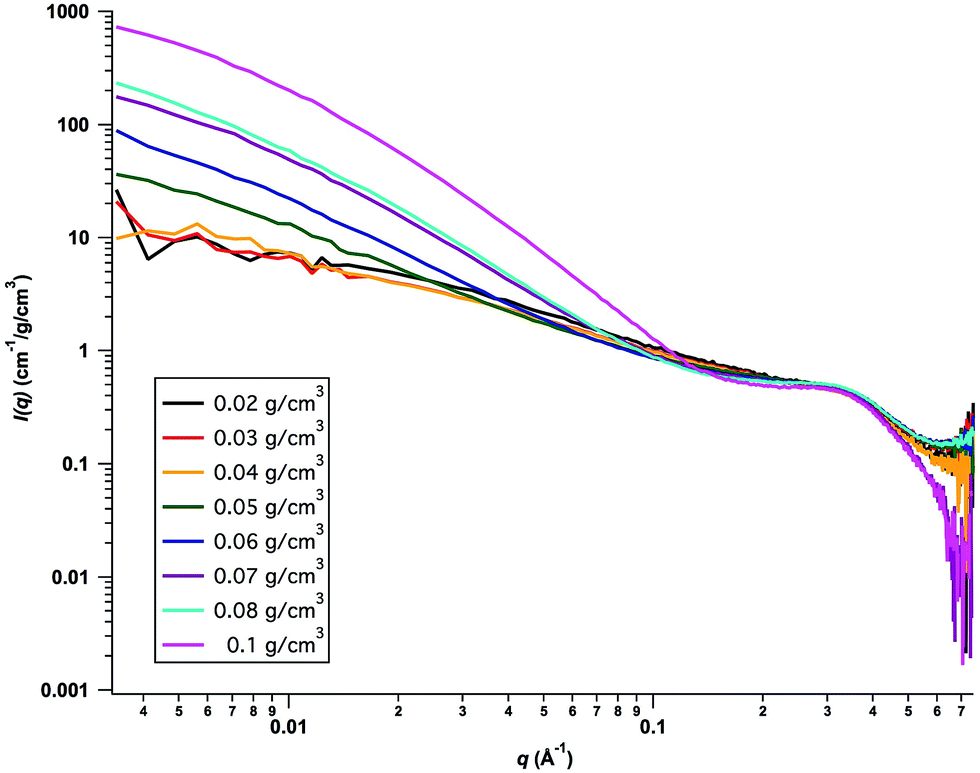
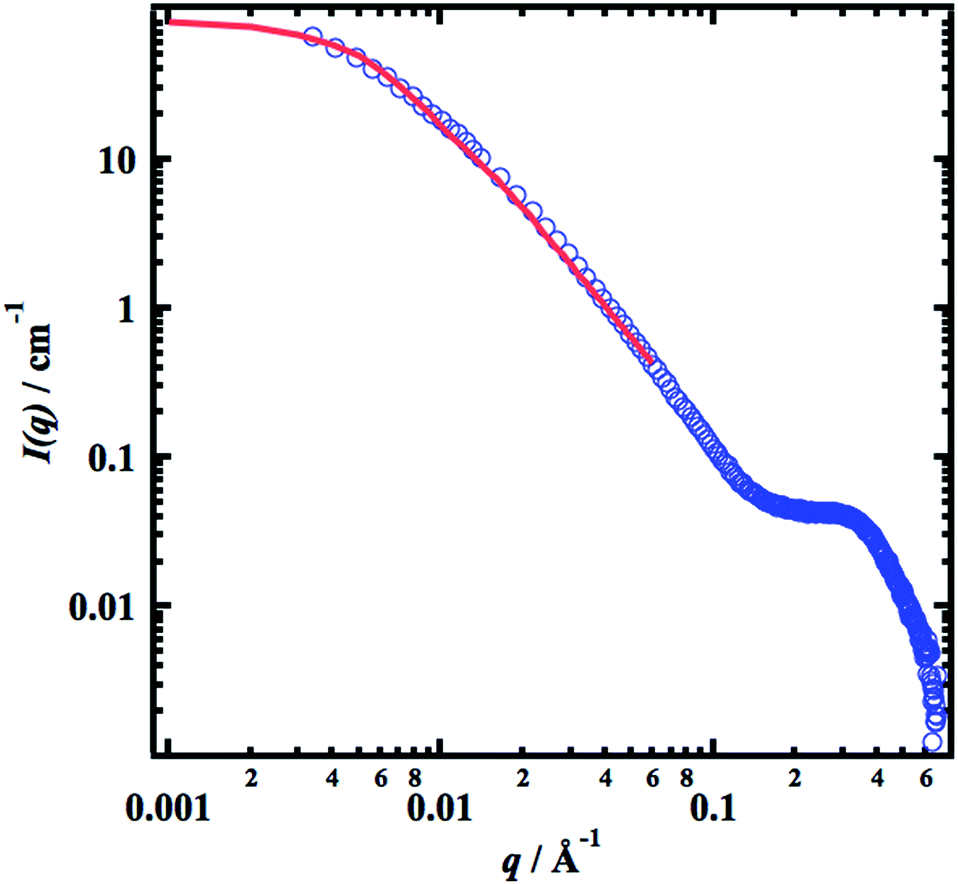
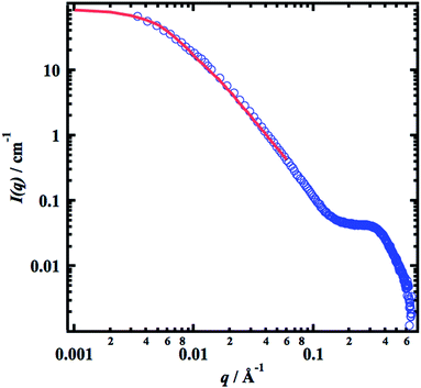
Small-angle X-ray scattering (SAXS) experiments were performed in the concentration range 0.02–0.1 g cm−3 of cellulose. The absolute scaled scattering profiles, normalized by the cellulose concentration (in g cm−3), are presented in Fig. 2. As can be seen, the data from the two lowest concentrations, 0.02 and 0.03 g cm−3, overlap in the whole q-range. At the highest q-values, q > 0.2 Å−1, the overlap remains for all concentrations, indicating that also for the highest concentration, 0.10 g cm−3, the cellulose is essentially fully molecularly dissolved.
 |
| | Fig. 2 Concentration normalized SAXS intensities, I(q)/c, versus q. Cellulose concentrations are indicated in the figure. | |
The bump observed in the scattering curves at q ≈ 0.35 Å−1 represents a characteristic feature of the average effective cross section of the cellulose chain. The scattering is consistent with a core–shell structure, having an overall diameter of approximately twice the size of a glucose monomer unit, and where the shell has a scattering length density, ca. 10% lower than in the bulk. As TBA+ has a slightly lower scattering length density than water, this is consistent with an excess concentration of TBA+ in the first solvation shell of the cellulose molecules. This can be due both to electrostatic attraction, because of the high pH, and to hydrophobic interactions. This preferential solvation by TBA+ ions is confirmed by recent self-diffusion experiments.16
We have modelled the SAXS data using the form factor, P(q), of semi-flexible chains with excluded volume interactions, obtained by Pedersen and Schurtenberger.17,18 The model form factor, parameterized from Monte Carlo simulations, captures the polymer coil at the different length scales, from the Guinier regime to the cross section structure of the chain. For the final cross section it makes use of the decoupling approximation
| | |
P(q) = Pchain(q)Pcs(q)
| (7) |
where
Pchain(
q) describes the average overall coil structure, which depends on the contour length,
L, and the persistence length
λp, and
Pcs(
q) is the cross section form factor. Light scattering data indicated repulsive inter coil interactions in dilute solution. A common approach to include excluded volume interactions in dilute solutions is the random phase approximation
19,20where the interaction strength parameter
υ = 1/
S(0) − 1.
In Fig. 3 we present the scattering curve from c = 0.02 g cm−3, together with a model based on eqn (4) and (5) in (3). The parameters used in the model calculation are c = 0.02 g cm−3, core radius Rcore = 5 Å, core scattering length density ρcore = 1.3 × 1011 cm−2, shell thickness tshell = 5 Å, shell scattering length density ρshell = 8.9 × 1010 cm−2, contour length L = 3000 Å (calculated from the molecular weight as L = (Mz/MAGU)lAGU, where MAGU = 162 g and lAGU = 5.15 Å are the molar mass and effective length of the anhydrous glucose monomer unit, respectively, and Mz/MAGU = 574 being the z-averaged degree of polymerization), persistence length λp = 25 Å, and the interaction strength, ν = 10.5. As can be seen, there is a good agreement between the model and experiment. c = 0.02 g cm−3 corresponds to approximately 0.7c*, where c* ≈ 0.03 g cm−3 is the overlap concentration as determined by rheology measurements,21 and the relative high value of ν, and correspondingly low value of S(0), comes from that upon approaching c*, higher order virial coefficients can no longer be neglected.
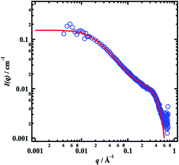 |
| | Fig. 3 SAXS pattern (blue circles) from a 0.02 g cm−3 sample together with a model calculation (red line). | |
Turning to higher concentrations, we see in Fig. 2 that from ca. 0.04 g cm−3 the normalized scattered intensity at lower q-values increases with increasing cellulose concentration. For the highest concentration, c = 0.1 g cm−3, the normalized intensity at lower q-values has increased by almost 2 orders of magnitude. The increase in low q scattering is denotative of effectively attractive interactions. Hence, there is a striking crossover from repulsive interactions to aggregation and effectively attractive interactions, occurring at approximately c = 0.04 g cm−3. There are two possible explanations for such a sudden onset of aggregation. Either it may be an equilibrium micelle formation, occurring within a homogeneous phase, or involve a phase transition and the formation of a new phase.22 Although cellulose is slightly amphiphilic,4 it is so only at the level of the monomer, and for a homopolymer, like cellulose, equilibrium micelle formation is unlikely. Most likely we are rather dealing with a phase transition and the onset of cellulose precipitation from a supersaturated solution.
Cellulose can crystallize in several different polymorphs, that are expected to have different solubilities. When synthesized in the plant cell wall, cellulose precipitates as cellulose I,23 with parallel chains. However, this crystal structure is metastable with respect to cellulose II, where the chains are anti-parallel, and which normally form when cellulose is recrystallized (regenerated) from solution.24 Cellulose II being more stable, with a lower cellulose chemical potential, compared to cellulose I, implies that cellulose II has the lower solubility of the two. A possible explanation for the behavior observed for c > 0.04 g cm−3 is thus that the cellulose I of the MCC dissolves and creates a solution that is supersaturated with respect to cellulose II, which then slowly precipitates. This scenario implies that the solubility of cellulose II is ca. 0.04 g cm−3, while the solubility of cellulose I is >0.1 g cm−3.
Polymer crystallization is a complex process and the solid phase is generally only semi-crystalline containing significant amounts of amorphous defect domains. As for small molecules, polymer crystallization is a nucleation and growth process.25,26 A significant difference between polymer crystallization and the crystallization of small molecules, however, is that polymer chains can participate in more than one nucleus. The nuclei are often referred to as fringed micelles27 and a cross linked network may arise, leading lead to gelation. Fringed micelles have also been proposed by Burchard and coworkers to describe the colloidal aggregate structure of cellulose and some derivatives.28,29 If now the cellulose II solubility is ca. 0.04 g cm−3, then more than half of the cellulose in a 0.1 g cm−3 sample should be in the precipitated solid phase at equilibrium. However, for the concentration range investigated here, c ≤ 0.1 g cm−3, solutions show no observable diffraction peaks in wide angle X-ray scattering.30 Neither were there any significant change in the SAXS pattern on the time scale of days. This apparent kinetic stability then suggests that we here are within the induction phase of the nucleation process where all nuclei formed are still sub-critical and unstable, and hence reversible and able to re-dissolve.
The onset of attractive interactions essentially coincides with the overlap concentration, c* ≈ 0.04 g cm−3. In the semidilute regime, where the polymer coils overlap, the scattering can no longer be described in terms of P(q) and S(q). The transient network is rather described in terms of a screening length, ξ, essentially corresponding to the network mesh size of the transient network.20 In a first attempt to model the observed low q scattering, we simply consider it as an excess scattering arising from a low concentration of, i.e. well separated, cellulose aggregates. We focus here only at lower q < ξ, and assume that the aggregates can be described as mass fractal clusters, having a radius of gyration, Rg,c, and fractal dimension, d. We use the corrected Beaucage model, as described by Hammouda31 where the normalized cluster form factor is given by
| |
 | (9) |
with
| |
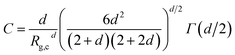 | (10) |
where
Γ(
x) is the gamma function. In
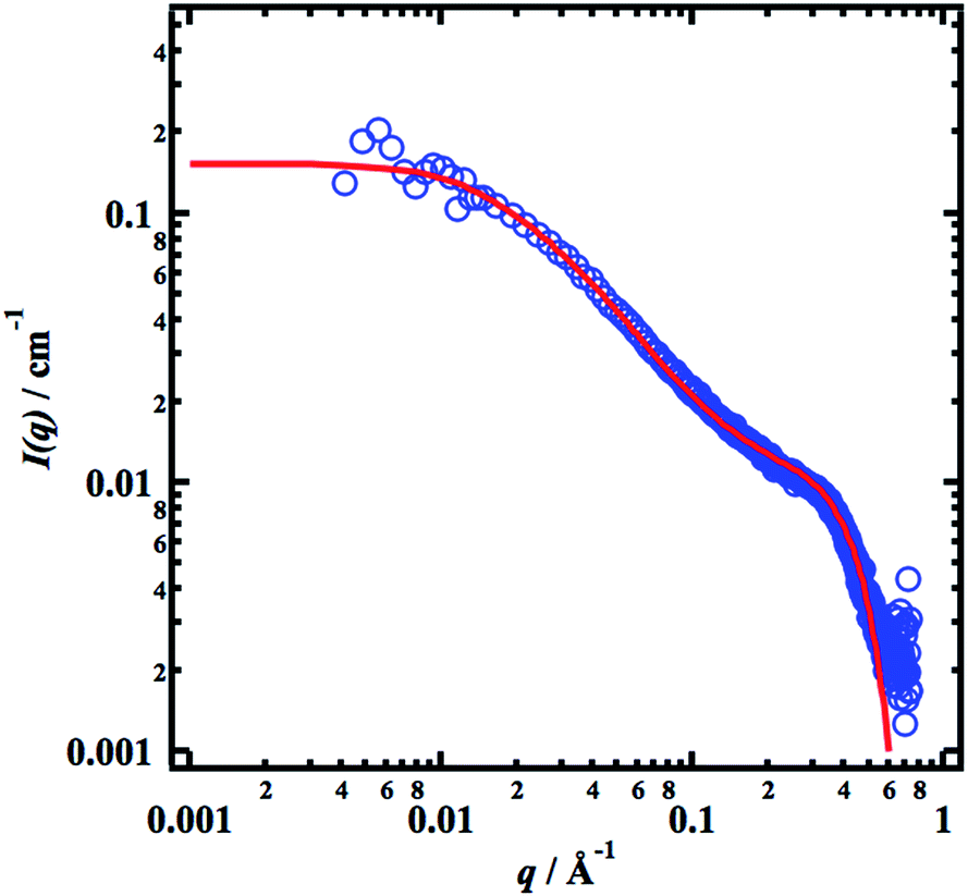
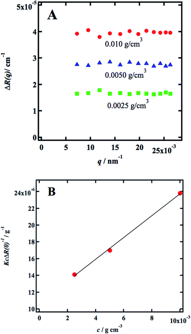
Fig. 4 we show the SAXS pattern of the 0.1 g cm
−3, sample, together with a simulated scattering curve
Ic(
q) =
Ic(0)
Pc(
q), with
Ic(0) = 85 cm
−1,
Rg,c = 270 Å and
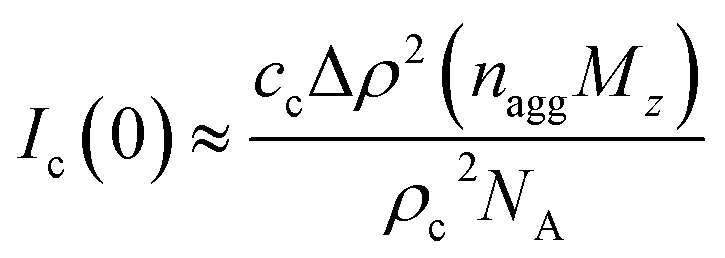
d = 2.2. The model is probably somewhat naïve, but it allows us to estimate some numbers. First,
Ic(0) is related to the average aggregation number,
nagg, of the clusters, and neglecting interactions we have
| |
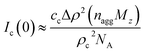 | (11) |
where
cc ≤
c is the concentration of cellulose that are involved in the clusters (
c is the total concentration of cellulose in the sample). With
Ic(0) = 85 cm
−1, we obtain
nagg ≈ 8
c/
cc. Hence if all cellulose chains are aggregated into clusters,
i.e. cc =
c, the average aggregation number
nagg ≈ 8. If
cc is smaller,
nagg is correspondingly larger. The
Rg,c value is larger than the corresponding value,
Rg ≈ (
Llp/3)
1/2 ≈ 160 Å, for the average single chain. Furthermore,
d is larger than 5/3, which is the effective fractal dimension of a single polymer coil, consistent with more densely packed aggregates.
 |
| | Fig. 4 SAXS pattern (blue circles) from a 0.10 g cm−3 sample together with a model calculation (red line, see text). | |
Conclusions
We have shown that microcrystalline cellulose (MCC) dissolved in 40 wt% THAH(aq) show repulsive interactions (good solvent conditions) at lower concentrations up to ca. 0.04 g cm−3. Above this concentration, cellulose aggregation is observed. We propose the possibility that 0.04 g cm−3 corresponds to the solubility of cellulose II, while the solubility of cellulose I is significantly higher. Thus dissolving MCC above 0.04 g cm−3 result in supersaturated solutions with respect to cellulose II that precipitates. SAXS data also indicate a preferential solvation of cellulose by TBA+ ions. This may be a significant ingredient in understanding cellulose solubilisation, possibly as a phenomenon of cosolvency.32
Acknowledgements
We thank Björn Lindman, Lars Stigsson, Luis Alves, Bruno Medronho, and members of the Avancell collaborative research program, supported by The Södra Foundation for Research, Development and Education, for interesting discussions and for introducing us to the problem of cellulose dissolution. We also thank Caroline Löfgren at Södra for providing SEC-MALS analysis of the cellulose source. We thank the Bo Rydin Foundation for Scientific Research and the Swedish Research Council for financial support.
Notes and references
- D. Klemm, B. Heublein, H. P. Fink and A. Bohn, Cellulose: fascinating biopolymer and sustainable raw material, Angew. Chem., Int. Ed. Engl., 2005, 44, 3358–3393 CrossRef CAS PubMed.
- J. L. Wertz, J. P. Mercier and O. Bédué, Cellulose Science and Technology, EPFL Press, Boca Raton, 1st edn, 2010 Search PubMed.
- B. Medronho and B. Lindman, Competing Forces During Cellulose Dissolution: From Solvents to Mechanisms, Curr. Opin. Colloid Interface Sci., 2014, 19, 32–40 CrossRef CAS.
- B. Medronho, A. Romano, M. G. Miguel, L. Stigsson and B. Lindman, Rationalizing Cellulose (in)Solubility: Reviewing Basic Physicochemical Aspects and Role of Hydrophobic Interactions, Cellulose, 2012, 19, 581–587 CrossRef CAS.
- T. Liebert, Cellulose Solvents – Remarkable History, Bright Future, in Cellulose Solvents: For Analysis, Shaping and Chemical Modification, ed. T. Liebert, T. Heinze and K. J. Edgar, American Chemical Society, Washington, DC, 2010; vol. 1033, pp. 3–54 Search PubMed.
- C. Woodings, Regenerated Cellulose Fibres, CRC Press LLC, Boca Raton, USA, 2001 Search PubMed.
- W. Wei, X. Wei, G. Gou, M. Jiang, X. Xu, Y. Wang, D. Hui and Z. Zhou, Improved Dissolution of Cellulose in Quaternary Ammonium Hydroxide by Adjusting Temperature, RSC Adv., 2015, 5, 39080–39083 RSC.
- M. Abe, Y. Fukaya and H. Ohno, Fast and Facile Dissolution of Cellulose with Tetrabutylphosphonium Hydroxide Containing 40 wt% Water, Chem. Commun., 2012, 48, 1808–1810 RSC.
- L. Alves, B. F. Medronho, F. E. Antunes, A. Romano, M. G. Miguel and B. Lindman, On the Role of Hydrophobic Interactions in Cellulose Dissolution and Regeneration: Colloidal Aggregates and Molecular Solutions, Colloids Surf., A, 2015, 483, 257–263 CrossRef CAS.
- L. Alves, B. Medronho, F. E. Antunes, D. Topgaard and B. Lindman, Dissolution State of Cellulose in Aqueous Systems. (1) Alkaline Solvents, Cellulose, 2016, 23, 247–258 CrossRef CAS.
- Neutron, X-rays and Light: Scattering Methods Applied to Soft Condensed Matter, ed. P. Lindner and T. Zemb, Elsevier, Amsterdam, 2002 Search PubMed.
- C. Löfgren, (private communication).
- A. A. Karimi, O. Dolotko and D. Dalmazzone, Hydrate Phase Equilibria Data and Hydrogen Storage Capacity Measurement of the System H2 + Tetrabutylammonium hydroxide + H2O, Fluid Phase Equilib., 2014, 361, 175–180 CrossRef CAS.
- H. Yamakawa, On the Theory of the Second Virial Coefficient for Polymer Chains, Macromolecules, 1992, 25, 1912–1916 CrossRef CAS.
- A. J. Barrett, Second Osmotic Virial Coefficient for Linear Excluded Volume Polymers in the Domb–Joyce Model, Macromolecules, 1985, 18, 196–200 CrossRef CAS.
- L. Gentile and U. Olsson, submitted.
- J. S. Pedersen and P. Schurtenberger, Scattering Functions of Semiflexible Polymers With and Without Excluded Volume Effects, Macromolecules, 1996, 29, 7602–7612 CrossRef CAS.
- W.-R. Chen, P. D. Butler and L. J. Magid, Incorporating Intermicellar Interactions in the Fitting of SANS Data From Cationic Wormlike Micelles, Langmuir, 2006, 22, 6539–6548 CrossRef CAS PubMed.
- H. Benoit and M. Benmouna, Scattering From a Polymer Solution at an Arbitrary Concentration, Polymer, 1984, 25, 1059–1067 CrossRef CAS.
- J. S. Higgins and H. C. Benoit, Polymers and Neutron Scattering, Oxford University Press. Oxford, 1994 Search PubMed.
- M. Gubitosi, L. Gentile, H. Duarte, U. Olsson and B. Medronho, unpublished.
- D. F. Evans and H. Wennerström, The Colloidal Domain: Where Physics, Chemistry, Biology and Technology Meet, John Wiley & Sons, Inc, New York, 2nd edn, 1999 Search PubMed.
- R. H. Atalla and D. L. VanderHart, Native Cellulose: A Composite of Two Distinct Crystalline Forms, Science, 1984, 223, 283–285 CAS.
- P. Langan, N. Sukumar, Y. Nishiyama and H. Chanzy, Synchrotron X-Ray Structures of Cellulose Iβ and Regenerated Cellulose II at Ambient Temperature and 100 K, Cellulose, 2005, 12, 551–562 CrossRef CAS.
- M. Muthukumar, Shifting Paradigms in Polymer Crystallization, in Progress in Understanding Polymer Crystallization, Lecture Notes in Physics, ed. G. Reiter and G. R.Strobl, Springer, Berlin, Heidelberg, 2007, vol. 714, pp. 1–18 Search PubMed.
- M. Muthukumar and P. Welch, Modeling Polymer Crystallization From Solutions, Polymer, 2015, 41, 8833–8837 CrossRef.
- A. Keller, Crystalline Polymers; An Introduction, Faraday Spec. Discuss. Chem. Soc., 1979, 68, 145–166 RSC.
- W. Burchard, Polymer Structure and Dynamics, and Polymer–Polymer Interactions, Adv. Colloid Interface Sci., 1996, 64, 45–65 CrossRef CAS.
- L. Schulz, B. Seger and W. Burchard, Structures of Cellulose in Solution, Macromol. Chem. Phys., 2000, 201, 2008–2022 CrossRef CAS.
- P. Nosrati, M. Koder Hamid, M. A. Behrens, J. Hagman, M. Gubitosi and U. Olsson, unpublished.
- B. Hammouda, Analysis of the Beaucage Model, J. Appl. Crystallogr., 2010, 43, 1474–1478 CrossRef CAS.
- J. Dudowicz, K. F. Freed and J. F. Douglas, Cosolvency and Cononsolvency Explained in Terms of a Flory–Huggins Type Theory, J. Chem. Phys., 2015, 143, 131101–131106 CrossRef PubMed.
|
| This journal is © The Royal Society of Chemistry 2016 |
Click here to see how this site uses Cookies. View our privacy policy here. 
 . The refractive index of 40 wt% TBAH(aq) was determined to be 1.406(3) and dn/dc 0.108 cm3 g−1 at ambient temperature.