The structure and dynamics of chitin nanofibrils in an aqueous environment revealed by molecular dynamics simulations

Abstract

Chitin is one of the most abundant structural biomolecules in nature, where it occurs in the form of nanofibrils that are the smallest building blocks for many biological structural materials, such as the exoskeleton of Arthropoda. Despite this fact, little is known about the structural properties of these nanofibrils. Here, we present a theoretical study of a single chitin molecule and 10 α-chitin nanofibrils with different numbers of chains in an aqueous environment that mimics the conditions in natural systems during self-assembly. Our extensive analysis of the molecular dynamics trajectories, including free energy calculations for every model system, reveals not only the structural properties of the nanofibrils, but also provides insight into the principles of nanofibril formation. We identified the fundamental phenomena occurring in the chitin nanofibrils such as their hydrogen bonding pattern and resulting helical shape. With increasing size, the nanofibrils become increasingly stable and their structural properties approach those of crystalline α-chitin if they consist of more than 20 chains. Interestingly, this coincides with the typical size of chitin nanofibrils observed in natural systems, suggesting that their evolutionary success was at least partially driven by these specific structure–property relations.

---

Introduction

In contrast to most man-made structural materials, biological materials are inherently structurally heterogeneous. Most of them consist of a matrix of structural biopolymers and various other organic components that are produced by the organisms themselves which control their formation and, either directly or indirectly, the formation of subassemblies which lead to the hierarchical organization of these materials. Among the known structural biopolymers, chitin is the second most abundant biopolymer in nature, after cellulose,¹ and forms the organic matrix in the cell walls of fungi and the exoskeletons of Arthropoda.² Arthropod exoskeletons are formed from the cuticle, a hierarchically structured fibre-based composite, where chitin is responsible for both shaping and reinforcing the material. The polysaccharide molecule chitin is a linear polymer of β-1,4 linked N-acetylglucosamine. The predominant form occurring in the cuticle is crystalline α-chitin, where the chains are arranged in anti-parallel fashion with a highly ordered orthorhombic symmetry that originates from hydrogen bonds of four hydroxyl groups and two amide groups in the repeating unit.^2–4 Two other forms of chitin found in nature are β-chitin and γ-chitin. β-Chitin can be found for example in squid pens.⁵ Its abundance is very low due to the parallel arrangement of chitin chains, which does not provide as strong a hydrogen bond pattern as in α-chitin. γ-Chitin has been described in insect cocoons or other special structures formed by insects,⁴ and it contains a repeating motif where two parallel chains are complemented by one in the opposite orientation.

Typical α-chitin crystallites occurring in the cuticle have a polygonal section profile and consist of 18–25 chitin molecules with a diameter between 2 and 5 nm and lengths of about 300 nm.⁶ They are always surrounded by a sheath of proteins, resulting in rod-shaped nanofibrils that have been identified as the basic structural unit of the cuticle in a large variety of species from all groups of Arthropoda.^6–9 Potential chitin-organizing proteins currently under discussion are a class of evolutionarily conserved cuticle proteins featuring the so-called Rebers and Riddiford (R&R) domain⁹ such as resilin, and the obstructor proteins¹⁰ that possess tachycitin-like chitin-binding domains. The long-known sterical compatibility between the amino groups of the acetylglucosamine and amino acid residues of the proteins have been proposed to facilitate the formation of hydrogen bonds between the molecules.¹¹ However, the exact functions of these proteins have not been identified yet. Chitin–protein nanofibrils further organize into stacks of planar arrays that form the so-called twisted plywood structure commonly found in all exoskeletal elements of Arthropoda. While the ground-state structure of α-chitin,^7,8,12,13 its mechanical properties and the impact on the overall mechanical performance of the composite cuticle have been extensively studied both theoretically and experimentally,^14,15 little is known about how it organizes to form the chitin–protein nanofibrils. During the process of cuticle formation,¹⁶ chitin molecules are produced by the membrane inserted enzyme chitin synthase.¹⁷ The enzyme catalyses the β-1-4 linkage between N-acetylglucosamines supplied from the cytoplasm. The formed chitin molecules are extruded across the plasma membrane into the extracellular space.^18–21 Here, the chitin and chitin-binding proteins present in the extracellular space organize into the typical nanofibrils that form the exoskeleton, most likely in a self-assembly process. This process involves the assembly of chitin molecules into larger fibrils and their interaction with chitin-binding proteins, which are the fundamental steps not only for the formation of the exoskeleton itself, but also establish the fundamentals that lead to the elaborate function-specific structural differentiation in the final tissue observed in many species of arthropods.

Even though crystalline α-chitin has been intensively studied in past years,^12,14,22,23 its structural properties remain unclear. Likewise experimental evidence concerning nanofibril composition, structural parameters and hierarchical structure were never further expanded to explain the self-organization of chitin nanofibrils. Since suitable in vitro and even more so in vivo experimental approaches are barely practicable in terms of elucidating the basic principles of the self-assembly of single chitin molecules to α-chitin nanofibrils, this study employs theoretical approaches using molecular dynamics in fully solvated systems to shed light on these processes. There are only few studies described in the past that employ molecular dynamics for description of chitin properties. For example, properties of a single chitin chain was studied by molecular dynamics approach in aqueous environment²⁴ and during adhesion to montmorillonite clay.¹ More complex studies try to describe adsorption of chitosan to chitin nanocrystallites,²⁵ thermodynamics of α-chitin de-crystallization,²⁶ and properties of chitin–protein composites.²⁷ Recently, a coarse grain model of crystalline α-chitin was derived from experimental data and atomistic molecular dynamics simulations.²⁸

However, to our best knowledge, none of these studies did characterize self-assembly of α-chitin nanofibrils and structures of possible intermediates in a comprehensive way. Due to methodological constraints, the self-assembly process of α-chitin nanofibrils in vivo as well as in vitro cannot be fully covered in an integral modeling experiment due to the size of simulated models, which are simply beyond current technical possibilities. Therefore, the process is studied in reverse by observing what the properties of already assembled chitin nanofibrils of various dimensions are.

Here, we evaluate the geometry of single chitin molecules and chitin nanofibrils of various sizes (Fig. 1), correlate the observed global structural features with local geometrical parameters, and analyze the driving forces responsible for the self-assembly of nanofibrils in terms of free energy changes. The studied nanofibril models were chosen such as to reflect successive intermediate fibril configurations that presumably occur during the self-assembly process leading to the nanofibril size reported in previous studies of arthropod cuticle.^29,30 This corresponds to the 6760 system (Fig. 1), which should be approximately 3 nm in diameter. Starting from the 6760 system, we considered one bigger and nine smaller systems. The shapes of smaller systems were selected in such a way that they reasonably span all important chain rearrangements in the both a and b crystallographic directions while avoiding simulations of too similar systems.

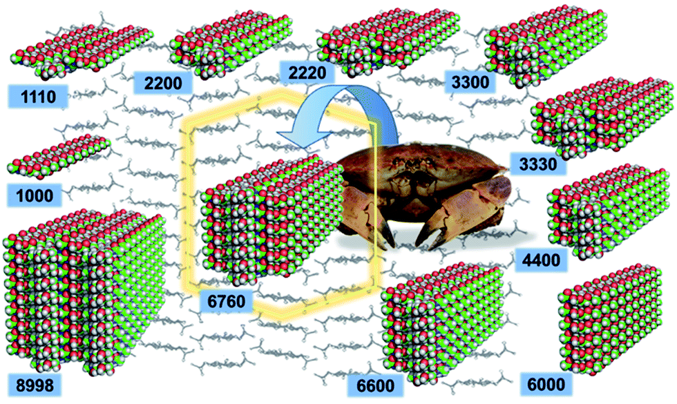Fig. 1 The eleven structural models of chitin nanofibrils analyzed in this study. Their denomination is based on the number of horizontally aligned chitin molecules (up to four), the numerical value of each digit indicates the number of vertically stacked molecules in the structure.

Materials and methods

Chitin nanofibril models were constructed in silico from the experimentally determined structure of an α-chitin crystal (Fig. 2).¹² Each model is composed of oligosaccharide chains of constant length. Each chain contains twenty units of N-acetylglucosamine (GlcNAc) linked by β-1,4 glycosidic bonds capped with hydroxyl groups on both chain terminals. The chains are then packed in the a and b lattice directions of the source α-chitin crystal, which preserves native contacts among individual chains, including both hydrophobic interactions as well as hydrogen bonds. These lead to either a single chain (1000) or fibrils in an antiparallel arrangement as combinations of 3 (1110), 4 (2200), 6 (2220, 3300, 6000), 8 (4400), 9 (3330), 12 (6600), 19 (6760) and 34 (8998) chains. The number of non-zero digits in the name is the number of chitin chains in the ab plane, whereas the numeral at a given position is the amount of chains in the corresponding ac plane. Detailed information about the simulated systems is provided in Table S1 in ESI (ESI†).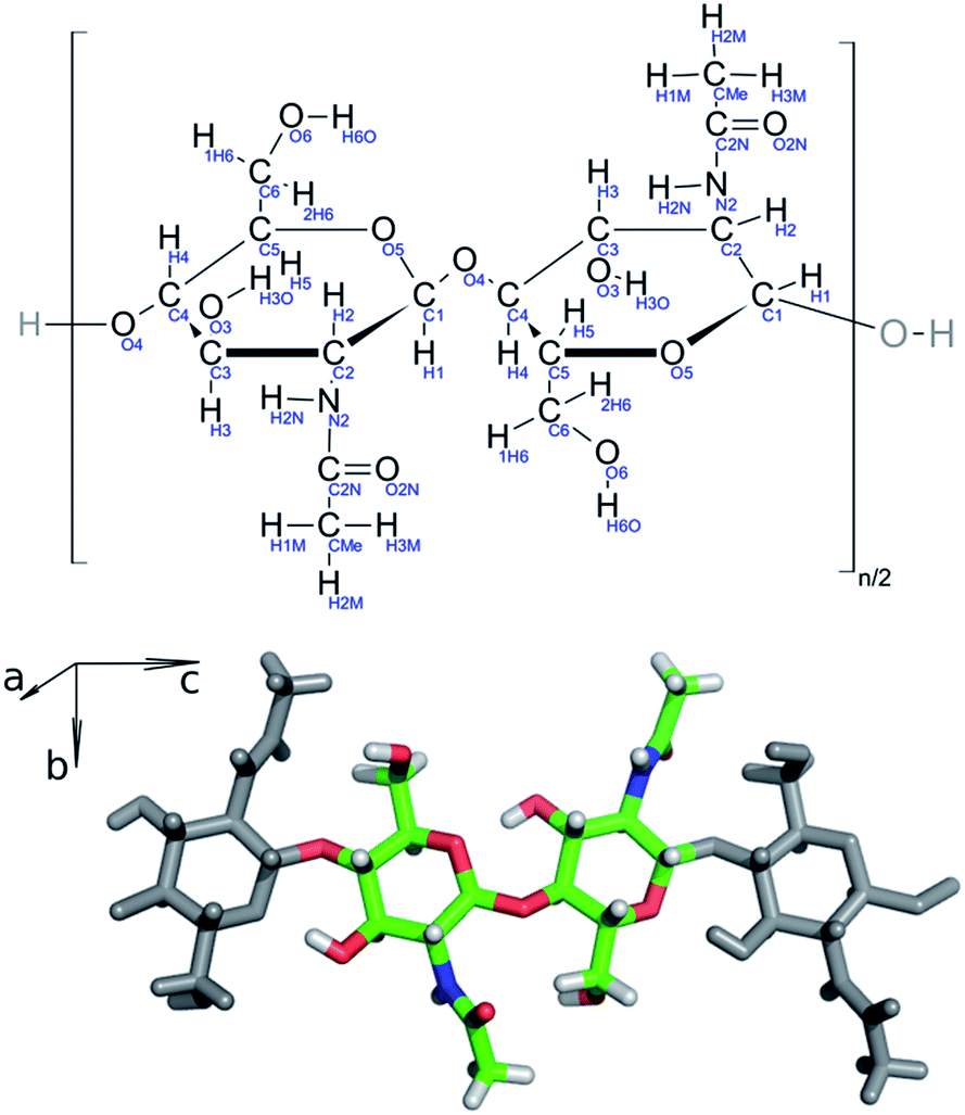

Fig. 2 (Top) Schematic structure of repeating N-acetylglucosamine dimers with atom names highlighted in blue. (Bottom) 3D structure of repeating N-acetylglucosamine dimers in a chitin chain, axes shown correspond to crystallographic axes.

Molecular dynamics simulations performed with the Amber 12 package³¹ were employed to evaluate the structural and dynamic behavior of the prepared models. The chitin nanofibrils were described with a GLYCAM 06g force field.³² To mimic the native conditions in the chitin nanofibril assembly zone, each structure was put in a truncated octahedral box, which was filled with water molecules described by the TIP3P water model.³³ Long-range interactions under the periodic boundary conditions were treated by the particle-mesh-Ewald method,³⁴ with a direct summation cut-off of 9.0 Å. The same cut-off distance was used for the treatment of van der Waals interactions. Each system was equilibrated prior to the production of simulations. The system was slowly heated from 5 K to 300 K. During the equilibration, the solute was kept fixed by positional restraints with decreasing strength from 50.0 to 0.0 kcal mol⁻¹ A⁻², with the initial structure used as a reference structure. The barostat set to 100 kPa was enabled at later stages of the equilibration to reach the proper density of the water environment.

Production simulations were performed at a constant temperature of 300 K and a pressure of 100 kPa. The lengths of all bonds containing hydrogen atoms were kept fixed, enabling an integration time step of 2 fs to be used. Temperature was kept fixed by Langevin thermostat employing a collision frequency of 1.0 ps⁻¹. Pressure was maintained by a weak coupling barostat with a feedback time constant of 1.2 ps. The production dynamics were run on GPU accelerators.³⁵ The length of each production run was 200 ns, configuration snapshots were taken each 10 ps.

Trajectory analyses were performed in the ptraj and cpptraj modules³⁶ of the Amber package or using in-house developed scripts. The root-mean square deviation (RMSD)³⁷ was calculated for each snapshot along the trajectory to the reference structure, which was the initial structure (e.g. crystal-like structure).

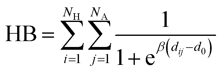
Hydrogen bonds were analyzed by evaluating number of contacts between the H and A atoms in patterns of the following form D–H⋯A–Z that might be considered as a stabilizing interaction, where the three dots denote the hydrogen bond.³⁸ The number of contacts was calculated using a Fermi switch function:

where d_ij is the distance between the hydrogen H and acceptor A atoms of analyzed contact. The β and d₀ parameters were chosen as 10.0 Å⁻¹ and 2.5 Å. These parameters are able to discriminate hydrogen bonds from long-range non-specific interactions for a varied range of hydrogen and acceptor atoms, as can be seen from a comparison of the switch function and histograms of the distances d_ij depicted in Fig. S1.† In our analysis, the directionality of a hydrogen bond is not taken explicitly into account. Thus in some cases, the obtained results might be contaminated by contacts that cannot be considered as strong hydrogen bonds, but rather electrostatic interactions. These situations are however rare as it is demonstrated in Fig. S2† showing distribution of angle θ(D–H⋯A) for selected hydrogen bonds. Majority of considered contacts have the angle higher than 110°, which is recommended minimum value for the hydrogen bond.³⁸ We also compared our approach with the traditional one, which is usually based on simple true/false consideration based on fulfillment of distance and angle criteria. Depending on the used criteria, our approach overestimates or underestimates the number of hydrogen bonds up to 25% or 5% for strict and weaker criteria, respectively (for details see Table S2†).

The axial chirality was described as the pseudo-dihedral angle α between four points. The second and third points are the centers of mass of the sugar rings aligned in the ab terminal planes. These two points represent the helical axis of nanofibrils. The first and fourth points are the centers of mass of the top-edge sugar rings (in the b direction). The geometry of glycosidic bonds was evaluated using the ψ(C5ⁿ, C4ⁿ, O4ⁿ, C1ⁿ⁺¹) and ϕ(C4ⁿ, O4ⁿ, C1ⁿ⁺¹, O5ⁿ⁺¹) dihedral angles. Rotamers of terminal CH–CH₂OH groups were monitored using the dihedral angle δ(C4, C5, C6, O6) and orientations of terminal CH₃CONH–CH groups were monitored using the dihedral angle ε(C1, C2, N2, C2N). Ring conformations were analyzed by measuring the ϕ and θ ring-puckering coordinates for sugar rings (C1, C2, C3, C4, C5, and O5) and pseudo-rings (O4ⁿ, C4ⁿ, C3ⁿ, O3ⁿ, O5ⁿ⁺¹, C1ⁿ⁺¹).³⁹

The binding strength between chitin chains was evaluated by means of the MM/PBSA^40–42 as implemented in Amber 12. The method is based on post-processing the trajectories obtained during production molecular dynamics to assess the absolute free energy of the solute (chitin nanofibril). The absolute free energy G is composed of two major contributions: (a) the free energy of the solute in vacuum G_vac for a solute configuration ensemble generated in the solvent and (b) the solvation free energy of the solute G_sol, representing the vertical transfer from vacuum to solvent (thus this energy does not include any deformation energy). The first term is calculated from the solute enthalpy H, which is taken as a time average of the total solute energies E_MM calculated by means of molecular mechanics (MM), and entropy S. The calculation of the entropy term will be discussed later in more detail.

G = G_vac + G_sol = H − TS + G_sol = 〈E_MM〉 − TS + 〈G^el_sol〉 + 〈G^ne_sol〉

The solvation free energy is composed of two contributions: electrostatic G^el_sol and non-electrostatic G^ne_sol. The electrostatic part was evaluated by employing a Poisson–Boltzmann (PB) method⁴¹ to describe the solvent implicitly. The PB method requires the definition of the atomic radii separating the interior and exterior of the system. In this work modified Bondi parameters⁴⁰ were used, together with an interior relative dielectric constant set to 1.0. The exterior relative dielectric constant was set to 80.0, which corresponds to water. The non-electrostatic contribution was calculated by employing a surface tension model using the solvent accessible surface area^43,44 with a default tension constant for the given atomic radii sets (0.0072 kcal mol⁻¹ A⁻²). Due to the computational complexity of the MM/PBSA, snapshots taken every 1 ns were included in the analysis of the last 150 ns.

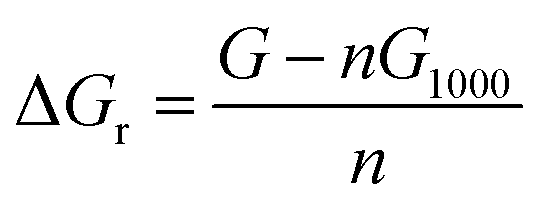
The change in the total reaction free energy related to a single chitin chain (the structure labeled 1000) was calculated via the following equation:

where G is the absolute free energy of the system containing n chitin chains, and G₁₀₀₀ is the absolute free energy of the 1000 system. The same equation was employed for the calculation of individual contributions to the total reaction free energy.

The essential dynamics analysis (EDA) method^45,46 was used to identify correlated atomic motions occurring during simulations. It is a post-processing method for molecular dynamics trajectories that can also be used to filter out thermal noise from analyzed trajectories. In the first step, the covariance matrix was calculated from fluctuations of the C1, C3, and C5 atoms around their average positions, employing trajectory snapshots taken every 10 ps. Then, eigenvalues and corresponding eigenvectors of the covariance matrix were evaluated. The eigenvalues represent the total mean square fluctuation of the system along the corresponding eigenvectors. Eigenvectors were employed to divide overall motion along the trajectory into separate modes. The modes with greater eigenvalues represent slow motion – essential motion, whereas modes with smaller eigenvalues represent rapid motion – thermal motion. New trajectories containing only correlated atomic motions individually projected from the source trajectory on five eigenvectors with the largest eigenvalues were calculated together with projection factors p.

For further analysis, the trajectories were coarse-grained. These simplified trajectories were employed in the vibrational entropy calculations. Each N-acetylglucosamine unit was represented by a point (CG bead) with a mass equal to the total mass of the N-acetylglucosamine unit, and its position was taken as the center of mass of all atoms in the given unit. The intention behind this procedure was to decrease the number of degrees of freedom while keeping the overall motions of systems close to representations with atomic resolution.

The entropy contributions were calculated separately for translation, rotation and vibrational motions using the cpptraj module from the Amber package. The translational S_t and rotational S_r contributions were calculated using statistical mechanical formulas for an ideal gas model at a temperature of 300 K and a pressure of 100 kPa. The vibrational entropy S_v was calculated for the same temperature using a quasi-harmonic approach.⁴⁷ To eliminate the impact of trajectory length on results, the vibrational entropy was calculated from varying blocks of the trajectory with lengths of 50 ns, 75 ns, and 150 ns and then extrapolated to infinite time.⁴⁸

Figures showing 3D structures of the studied systems were prepared in PyMol⁴⁹ and VMD.⁵⁰

Results and discussion

In the natural system, the pH and the ionic composition of the aqueous fluid present in the ecdysial gap where chitin nanofibrils assemble is controlled by the cells.⁵¹ Within our model environment, the experimentally determined low concentrations of Na⁺, K⁺, Mg²⁺, and Ca²⁺ ions in the moulting fluid of the crustacean Porcellio scaber during initial cuticle formation would have resulted in very few ions present in the simulation box. Since preliminary simulations in isotonic solution yielded similar results, all models were simulated in a water environment without the presence of any ions. Due to computational demands, the sizes of the models had to be kept reasonably small. The length of chitin chains was limited to twenty N-acetylglucosamine units, which corresponds to approximately 10.6 nm-long chains. This is about 30 times smaller than the reported length of chitin nanofibrils occurring in nature. However, the models are long enough to avoid artificial interactions between terminal sides in the axial direction. The average structures of our nanofibril model systems obtained from the entire production MD trajectories are shown in Fig. 3. It is immediately obvious that an increasing number of chitin chains in the a and b directions have a strong impact on the resulting overall structure of individual nanofibrils.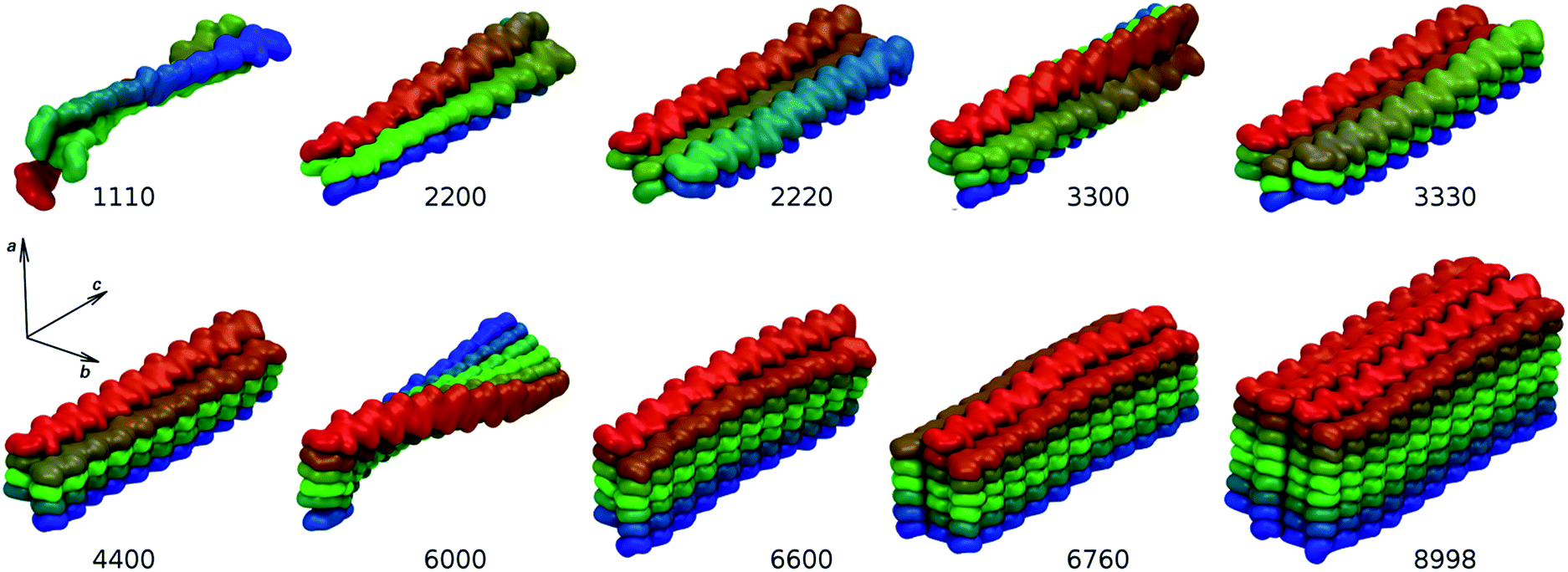

Fig. 3 Average structures of simulated nanofibril systems. Building blocks are color-coded to highlight structural features.

The overall flexibility of the different nanofibril models was monitored by root-mean square deviation (RMSD, Fig. 4 and S3†). This property quantifies the structural deviation of the simulated models from ideal, crystal-like structures. The larger this value is at a given time, the more the model structure deviates from the initial structure. The single chitin chain exhibits a broad fluctuation ranging from 3.3 to 15.1 Å, with a maximum at 5.3 Å. This indicates that the structure is rather flexible. Despite this fact, the structure maintains a straight shape without tendencies to fold into more compact structures. This was expected, as the single chitin chain would be the most flexible due to the lack of surrounding partners that would stabilize the structure. Surprisingly, it was found that some of the larger nanofibrils, namely the 1110, 2200, 6000, 6600 systems, deviate even more from the crystalline configuration, indicating an even higher flexibility. To explain this observation, the hydrogen bond network in nanofibrils was analyzed, as this is thought to be one of the key interactions that influence their shape, stability and mechanical properties.

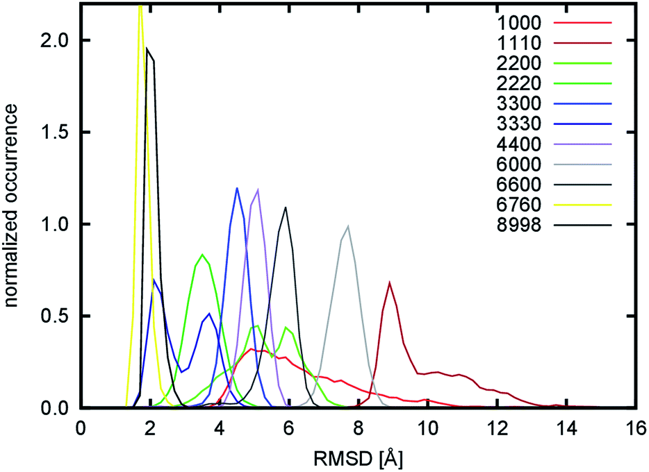Fig. 4 Distribution of RMSD.

The hydrogen bond analysis was performed for specific and non-specific pairs of hydrogen bond donor and acceptor atoms. The specific hydrogen bonds represent geometrically necessary interactions occurring in the crystalline α-chitin while the non-specific hydrogen bonds represent possible interactions that might coincidentally occur during its evolution or its deformation. The specific hydrogen bonds are represented by the O2N–H2N, O5–H3O, O2N–H6O, and O6–H60 atom pairs, and their statistics are summarized in Table 1.

Table 1 Statistics of specific hydrogen bonds^a

System	n	l	O5–H3O			O2N–H2N
			〈HB〉	σ(HB)	〈HB〉/n	〈HB〉	σ(HB)	〈HB〉/l
a n – number of chitin chains; l – number of stacking layers; 〈HB〉 – average number of hydrogen bonds; σ(HB) – variance (fluctuation) of number of hydrogen bonds; 〈HB〉/n – average number of hydrogen bonds related to a single chitin chain; 〈HB〉/l – average number of hydrogen bonds related to a single stacked layer of chitins.
1000	1	0	14.04	1.74	14.04	0.00	0.03	—
1110	3	0	44.01	2.76	14.67	2.04	1.12	—
2200	4	2	71.76	1.76	17.94	36.11	1.62	18.06
2220	6	3	110.00	1.64	18.33	56.18	1.61	18.73
3300	6	4	110.70	1.50	18.45	72.87	1.92	18.22
3330	9	6	166.40	1.72	18.49	113.40	2.19	18.90
4400	8	6	146.80	1.90	18.35	108.50	2.70	18.08
6000	6	5	109.00	1.87	18.17	89.91	2.64	17.98
6600	12	10	221.30	2.13	18.44	182.10	3.66	18.21
6760	19	16	353.40	2.03	18.60	308.30	3.07	19.27
8998	34	30	634.00	2.52	18.65	567.30	5.22	18.91

---

System	n	l	O2N–H6O			O6–H60
			〈HB〉	σ(HB)	〈HB〉/n	〈HB〉	σ(HB)	〈HB〉/l
1000	1	0	0.01	0.08	—	0.05	0.18	—
1110	3	0	9.01	4.12	—	3.24	1.52	—
2200	4	2	9.13	2.65	4.56	10.89	4.29	5.45
2220	6	3	13.48	2.92	4.49	13.48	2.92	4.49
3300	6	4	18.66	3.32	4.67	31.79	2.95	7.95
3330	9	6	28.63	4.00	4.77	59.01	3.91	9.84
4400	8	6	26.09	3.99	4.35	44.27	4.49	7.38
6000	6	5	16.19	3.78	3.24	12.53	2.77	2.51
6600	12	10	45.63	5.85	4.56	67.58	5.90	6.76
6760	19	16	89.73	5.92	5.61	143.50	7.07	8.97
8998	34	30	192.70	9.57	6.42	266.30	10.19	8.88

---

The largest number of hydrogen bonds per chain was detected for the O5–H3O atom pair. This type of hydrogen bond is responsible for stabilization along the c-axis of a single chitin chain due to an interaction between the O5 atom and H3O–O3 hydroxyl group from adjacent sugar rings. Except for the 1000 and 1110 fibrils, all systems exhibit values that range from 17.9 to 18.6. These values are close to the theoretical limit, which is 19.0 for twenty-unit-long chains. The 1000 and 1110 systems exhibit only slightly smaller values (about 14). These might be caused by the absence of stabilizing adjacent chitin chains in the ac plane, and the resulting complete exposure of both systems to the water environment. These hydrogen bonds are also responsible for the formation of seven-membered pseudo-rings, which are roughly in the chair conformation. Together with the sugar rings, which are also in the chair conformation, they form a thermodynamically stable belt-like structure of mutually interconnected rings. This arrangement makes single-chitin chains resistant to axial rotations along glycosidic bonds, which prevents a short single chain collapsing into a more compact structure. This is in agreement with the behavior observed in the simulation of the 1000 system. The conformation of rings was further quantified by the ring-puckering ϕ and θ angles (Fig. S4 and S5†). The polar θ angle is close to 180.0° for both kinds of rings, which correspond to the observed chair conformation. The azimuthal ϕ angle shows different distributions for every simulated system, but as the polar θ angle is always close to 180.0°, these changes actually reflect only very small geometrical changes. The only significant deviation of the polar θ angle from its ideal value of 180.0° was observed for the 1000, 1110, 2200, and 6000 systems. In these systems, the ring enclosures formed by the O5 and H3O atoms are not buried in the structure, but located on the surface and thus fully exposed to water, making the enclosures significantly weaker.

The second most common type of hydrogen bond is formed between stacked chitin chains (in the a direction) by interaction between the carbonyl O2N and amide H2N atoms. The number of hydrogen bonds per number of stacked layers is between 17.98 and 19.27, which is close to the theoretical limit of 20.0. The value slightly increases with an increase in the number of adjacent stacked layers in the b direction. For example, the 2200 system exhibits a value of 18.06, while the 2220 system exhibits a value of 18.73. However, this effect is less pronounced if the number of layers stacked in the a direction increases (see the 3300, 3330 and 6000, 6600 systems). From previous studies⁵² it follows that this type of hydrogen bond is responsible for maintaining the structural integrity of chitin crystallites in the a direction, which is in agreement with the behavior observed in all our simulated systems that contain stacked chains.

The remaining specific hydrogen bonds are formed by the O2N–H6O and O6–H60 atom pairs. Their values, related to either the number of chains or the number of stacked layers, are not as constant as in the two previous cases (Table 1), but strongly depend on the nanofibril size and shape. One possible explanation for this might be that these hydrogen bonds are weaker than the previous ones and could thus be influenced by the water environment at the surface of the nanofibrils. To confirm this hypothesis, we tried to rationalize this observation by including the effect of the solvent into the model. Instead of entering the number of hydrogen bonds purely due to the total number of stacked layers, the stacked layers were counted separately for the situation where they are exposed to the solvent (they are close to the surface of the nanofibril – l_w) or when they are located inside the nanofibril (l_i). To make the model robust, each edge of stacked layers was counted independently. The relationship was then considered as a simple linear model of the following form:

〈HB〉 = n_wl_w + n_il_i

where n_w and n_i are the number of hydrogen bonds per given stacked layer edge that need to be determined for layers exposed to water or the nanofibril internal environment, respectively. This simple model does not consider all contacts with water properly, for example on the ab and ac facets of the nanofibrils. Nevertheless it performed very well, as the square of the Pearson correlation coefficient (R²) between the number of hydrogen bonds obtained from the analyzed trajectories and that predicted by the model, found by the least-square fitting approach, is in both cases higher than 0.99 (Table S3, Fig. S6†). For the O2N–H6O hydrogen bond, the found parameters are 1.04 ± 0.35 and 3.92 ± 0.18 for n_w and n_i, respectively. For the O6–H60 hydrogen bond, they are 1.64 ± 0.61 and 5.57 ± 0.31, respectively. Indeed, these values confirm that the O2N–H6O and O6–H60 hydrogen bonds are weakened by the presence of the solvent, because in both cases the parameter n_w is about a third of n_i.

We also focused on the analysis of other possible hydrogen bonds that do not commonly occur in crystalline chitin. The aim was to find possible correlations between the presence of such non-specific hydrogen bonds and the observed structural shape of the simulated nanofibrils. However, the analysis of the O6–H3O, O6–H2N, O3–H6O, O3–H2N, O2N–H3O atom pairs did not confirm such correlations, as the number of these hydrogen bonds related to a single chain is negligible (smaller than one in all cases except for the 1110 system, see Table S4†).

During the simulation of the 1110 model system, we observed a structural reorganization of the nanofibril. This is characterized by a very large change in the RMSD, the largest observed deviation among all the tested systems. The RMSD shows a broader distribution in the range from 5.7 to 15.7 Å with a maximum at 8.9 Å (Fig. 4) for the 200 ns-long simulation. Detailed analysis of the trajectory showed that the structure of the model underwent a rearrangement, in which the non-covalent (mostly dipole–dipole) interaction between adjacent chains in the b direction is disrupted. This occurred during the equilibration stage of the simulation, which indicates that this kind of interaction is very weak and was the reason for their replacement with hydrogen bond interactions. To quantify this process, the evolution of emerging hydrogen bonds (HB) over time was calculated (Fig. 5). During the 200 ns-long simulation, we observed a sudden change in the structure of the nanofibril chain, which motivated us to extend the simulation to 500 ns to observe possible further reorganization. The hydrogen bonds were monitored for the O2N–H2N, O2N–H6O, and O6–H6O atom pairs as representatives of those specific hydrogen bonds. The evolution of the fourth specific hydrogen bond for the O5–H3O atom pair is not shown, since the count was constant throughout the whole simulation (around 44.1, see Table 1). The evolution of non-specific hydrogen bonds formed by the O6–H2N and O2N–H3O atom pairs was also monitored.

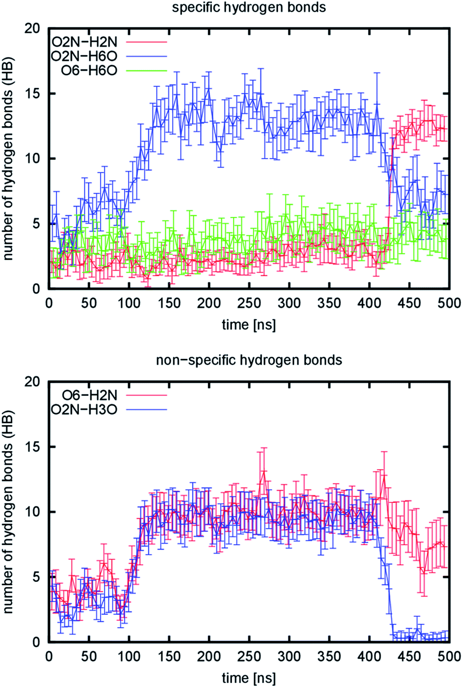Fig. 5 Number of hydrogen bonds emerging during simulation of the 1110 model. Lines represent running averages over 5 ns time intervals and vertical bars are variances in the same time interval.

Two changes occurred during the simulation: the first one happened in the interval from the 100^th to 150^th ns and the second change, which was more rapid, at about the 425^th ns. These two changes split the simulations into three regions, for which representative structural snapshots are shown in Fig. S7.† During the first change, the structure that still resembled the starting structure collapsed and became more compact, which resulted in an increase in the number of hydrogen bonds, especially non-specific ones. From the specific hydrogen bonds, only the O2N–H6O type prevails. However, a very slow increase in two other types is also visible in the region from the 150^th to 400^th ns. The average increase is 0.29 and 0.28 hydrogen bonds per 100 ns for the O2N–H2N and O6–H6O atom pairs. The second change is accompanied by an increase in the number of O2N–H2N hydrogen bonds. This resulted in the formation of regions in the structure where the chains change their position to the stacked conformation (Fig. S7,† highlighted with ovals). This stacking is not perfect yet, as the chains are not properly aligned vertically in some parts (they are slightly displaced relative to each other in the c direction). In addition, the chains even cross each other and stack in an inappropriate order in one part of the structure. Taken together, the observed changes suggest that the 1110 system slowly transforms into the 3000 system, where the stacking is the most dominant interaction due to specific hydrogen bonds. From the analysis of hydrogen bonds in the other simulated models, we can predict the numbers of hydrogen bonds for the 3000 arrangement to be: 36.44 (O2N–H2N), 4.16 (O2N–H6O), and 6.56 (O6–H6O). The number of non-specific hydrogen bonds should be close to zero. At the end of the 1110 simulation, the final values were: 12.29 (O2N–H2N), 7.25 (O2N–H6O), 3.83 (O6–H6O), and 7.33 (O6–H2N). From the comparison of the predicted and current value of the leading structural descriptor (O2N–H2N), we can assume that the transformation is approximately in the first third. The further rearrangement must involve the structure re-folding due to misaligned stacking. This was the reason why we did not continue with the simulation, because a significantly longer simulation time would be required.

The other simulated systems did not undergo any significant rearrangements like the one observed for the 1110 system. However, some of them still deviated significantly from the crystal-like geometries. This is especially noticeable for the 2200, 6000, and 6600 systems. The cause of this behavior is a twist distortion along the c-axis of the structure (see Fig. 3). This distortion makes all the systems axially chiral (in addition to the configurational chirality introduced by the stereogenic centers in the building saccharide units). As a measure of axial chirality, the pseudo-dihedral angle α was calculated and its distribution is shown in Fig. 6. Its average values, including the corresponding fluctuations, are summarized in Table 2.

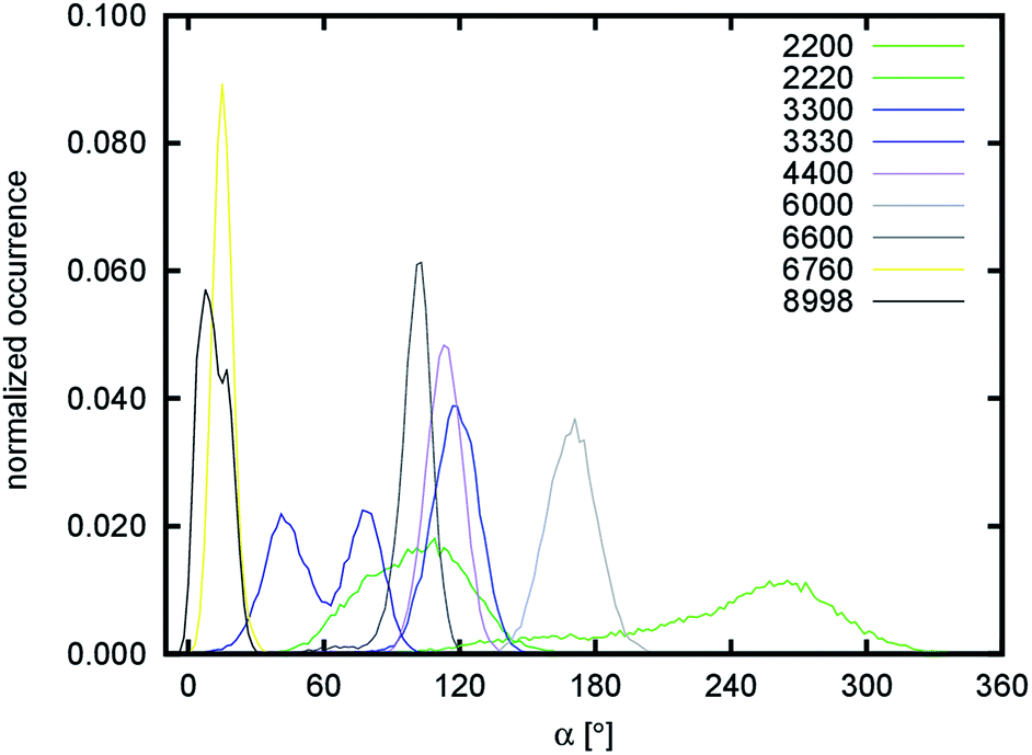Fig. 6 Distribution of pseudo-dihedral angle α quantifying axial chirality of nanofibril chains.

Table 2 Average values of dihedral angles α, ψ and ϕ and their root mean square fluctuations σ

System	〈α〉	σ(α)	〈ψ〉	σ(ψ)	〈ϕ〉	σ(ϕ)
1000	—	—	−129.0	20.5	−78.0	11.1
1110	—	—	−130.6	22.4	−79.1	10.8
2200	236.2	48.9	−139.7	10.5	−83.4	8.2
2220	100.3	22.5	−145.0	9.7	−86.8	7.8
3300	117.7	11.0	−145.5	9.1	−86.2	7.5
3330	59.2	19.9	−148.0	8.4	−88.0	7.2
4400	112.4	10.8	−146.4	8.9	−86.2	7.1
6000	169.4	11.4	−142.7	9.6	−85.3	7.5
6600	99.9	9.0	−146.9	8.5	−86.6	7.1
6760	15.4	5.8	−149.9	7.3	−89.1	6.7
8998	11.3	6.3	−150.9	7.8	−89.2	7.1

---

The factor that influences the degree of axial chirality most significantly is the number of stacked layers of chitin chains interacting in the b direction. The axial chirality decreases when a nanofibril is growing in this direction (compare the 2200 → 2220, 3300 → 3330, and 6000 → 6600 systems). The highest axial chirality among the simulated systems is exhibited by the 2200 and 6000 systems. The helical twist of 180° along the entire length is particularly obvious in the average structure of the 6000 system shown in Fig. 3. In an attempt to explain this behavior at the molecular level, we focused on possible correlations of the pseudo-dihedral angle α with different structural descriptors (Fig. S8–S10 and Tables S5 and S6†).

The significant correlation between the pseudo-dihedral angle α and structural descriptors was found for dihedral angles describing the geometry of the glycosidic bonds. The dihedral angles ψ and ϕ exhibit single Gaussian distributions (Fig. S9†). The peak maxima (average values) (Table 2) then correlated well with the pseudo-dihedral angle α with R² of 0.97 and 0.99, respectively. The obtained linear models (Fig. S10†) enable the extrapolation of ψ and ϕ to α = 0, which should correspond to the situation in crystalline α-chitin (no axial chirality is observed in the crystal). The comparison of the obtained values with the data extracted from two available crystal structures and ab initio calculations is summarized in Table 3. Although the values ψ and ϕ were not determined for the real structure of crystalline α-chitin, but extrapolated from the behavior of smaller chitin nanofibrils, their correspondence with the experimental as well as ab initio data is very good. They are approximately in the middle between two values determined by X-ray crystallography and are also close to the values determined by ab initio calculations. This can be taken as a performance validation of the force field employed for the description of chitin nanofibrils.

Table 3 Comparison of dihedral angles ψ and ϕ

	This work	Ab initio ^52	exp^8	exp^57
ψ	−151	−156	−142	−168
ϕ	−89	−97	−102	−73

---

We also checked if the observed agreement between our simulations, experimental, and ab initio data cannot be consequence of specific force-field parameters that would force the system to adopt configuration with values of the ψ and ϕ dihedral angles equal to values found by the extrapolation. We found that minima on the potential energy surface describing rotation on both glycosidic bonds do not coincide with the extrapolated values of dihedral angles (Fig. S11†). This indicates that observed behavior is a result of orchestration of all type of interactions among them dihedral, electrostatic and van der Waals interactions playing predominant role.

The twist was also observed in simulations of cellulose nanofibrils.^53–56 However it was shown that on longer timescales (∼800 ns) the twist can disappear due to reorganization of hydrogen bonds that starts at the solvent/solute boundary and slowly propagates into the body of cellulose nanofibril. Moreover it was shown that the phenomena is force-field dependent.⁵⁴ On timescale of our simulations (∼200 ns) we did not observe such disappearance of the twist. Splitting of distribution of the pseudo-dihedral angle α in the 3330 as well as 8998 systems (Fig. 6) is rather caused by an increase of the twist for a short period during the simulations. To further support this different observation, we extended length of simulation for 6000, 4400, and 6760 systems up to 300 ns (Fig. S12†). Once again, no sudden change or decrease in the twist was observed.

A recent study from the same authors performed on cellulose nanofibrils of various sizes and on shorter timescales (∼200 ns)⁵⁵ shows results that are very similar to our work. They found that the twist is decreasing with increasing size of nanofibril. Nevertheless they were not able to recognize that magnitude of the twist might exhibit anisotropy due to size of nanofibrils along the a and b directions because their nanofibrils were symmetrical. Also the molecular origin of the twist will be probably different as the authors identified HO2 group as a key player, which is however absent in chitin as this position is occupied by the N-acetylamide group.

Another correlation was found between the pseudo-dihedral angle α and average values of the ring-puckering coordinate θ for the pseudo-rings formed by the hydrogen bonds between the O5–H3O atom pairs. As a consequence, the pseudo-dihedral angle also correlates with the number of O5–H3O hydrogen bonds per chain (Table S6†). R² is 0.95 and 0.94, respectively.

The correlations found indicate that the twist distortion of the simulated nanofibrils is a consequence of the internal axial chirality of individual chitin chains. The internal axial chirality is caused by deviations of the ψ and ϕ dihedral angles from their ideal values observed in the crystal structure. In our model, these extrapolated ideal average values are −151.0° and −89.4°, while in the single chitin chain (the 1000 system) they are only −129.0° and −78.0°, respectively. The internal axial chirality of single chains is suppressed in larger chitin nanofibrils by non-covalent interactions between adjacent stacked layers of chitin chains. These probably include dipole–dipole interactions between acetamide groups in the b direction. As a consequence of distortion along glycosidic bonds, the number of O5–H3O hydrogen bonds that stabilize a belt-like structure of chitin chains was also found to correlate well with the overall axial chirality, together with the θ puckering coordinate describing such pseudo-ring conformations.

The axial chirality of chitin nanofibrils is also reflected in key soft-mode movements detected by the essential dynamics analysis of coarse-grained trajectories employing the C1, C3, and C5 atoms. This analysis separates the overall dynamic motion into linearly independent motions scored by their softness (e.g. how the energy of the system changes with the particular movement). Projections of the trajectories to the five essential modes with highest (softest) eigenvalues are summarized in Fig. S13.† Non-uniform (Gaussian) distributions of projections were found for several systems (most notably for 1110, 2200, 3330, 6600, and 8998). This indicates that the motion is too slow to be properly sampled on the timescale of the analyzed simulations. With the 1110 system, the non-uniform distributions of several modes are caused by the complex structural rearrangement, which was already discussed. With the 2200, 3330, 6600, and 8998 systems, the non-uniform distribution is caused by slow axial distortion, which is also visible in the distribution of the pseudo-dihedral angle α (Fig. 6, most notably the split distribution for the 3330 system).

The slowest essential modes show changes in the axial chirality for all systems (apart from 1000 and 1110), indicating that a twist distortion is energetically the most favorable deformation (Fig. 7, M1). The other modes show various types of distortion along the c direction, with the 6760 system they are variants of shear distortions (Fig. 7, M2). Since the 6760 system most closely resembles the geometry of chitin nanofibrils observed in arthropod exoskeletons, these properties might be important for the interaction between chitin nanofibrils and chitin-binding proteins in natural systems. While chitin is very stiff in the c direction due to the covalent nature of glycosidic bonds supported by the hydrogen bond network, it is rather soft in the other directions, which might facilitate small structural adjustments that enable proper alignment to the protein binding sites in living systems.

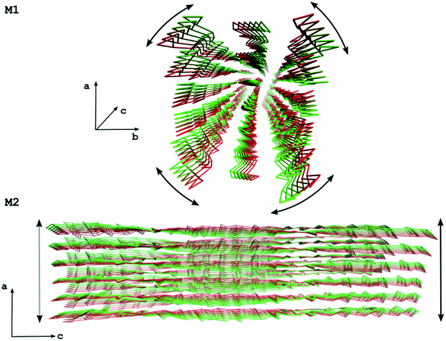Fig. 7 Movements along two essential modes for the 6760 system. The M1 mode shows a twist distortion while the M2 mode shows a shear distortion.

The fact that the chitin fibrils in mature and developing exoskeleton are always confined by various chitin-binding proteins makes it difficult to obtain direct experimental evidence for axial chirality in the α-chitin nanofibrils, since the interactions between chitin and proteins are likely to influence the structural conformation of the chitin fibrils. However, synchrotron X-ray micro-diffraction experiments have shown that in arthropod exoskeletons the crystallographic axes a and b of the chitin fibrils rotate around the longitudinal axis c.⁵⁸ This supports our results, since this rotation might very well originate from an initial axial distortion of the newly assembled chitin nanofibrils which is retained despite the addition of the protein coating.

The self-assembly of chitin chains into chitin nanofibrils is controlled by the kinetics and thermodynamics of individual assembly steps. The kinetics of self-assembly is very hard to describe by means of computational techniques, as the process is composed of several reaction pathways which are difficult to capture and characterize. An example of such a process partially occurred in the simulation of the 1110 model. In contrast, thermodynamics can be easily described by means of various computational techniques. In this work, we selected the MM/PBSA method. Using this method, we calculated the reaction free energies released during nanofibril formation.

The changes in reaction enthalpy in the gas phase ΔH_r/n show that the process is strongly exothermic. As we use molecular mechanics (pair-wise additive approach) to describe the system, it is possible to further decompose the enthalpy into individual energy terms (Table S7,†Fig. 8 and S14†). From the decomposition, it follows that the major driving forces in the binding are equally contributing electrostatic and van der Waals forces. This is very surprising, as we expected that the electrostatic contribution would be the major player due to the emerging hydrogen bond network and dipole–dipole interactions of acetamide groups. The value of ΔH_r/n decreases with an increasing number of chains to the limiting value (extrapolated for an infinite number of chitin chains), which we estimated to be about −651.1 ± 58.4 kcal mol⁻¹. This behavior was expected, because with an increasing number of chitin chains the nanofibril structures approach the structure of crystalline chitin (the ideal structure) where the overall interaction network is maximized.

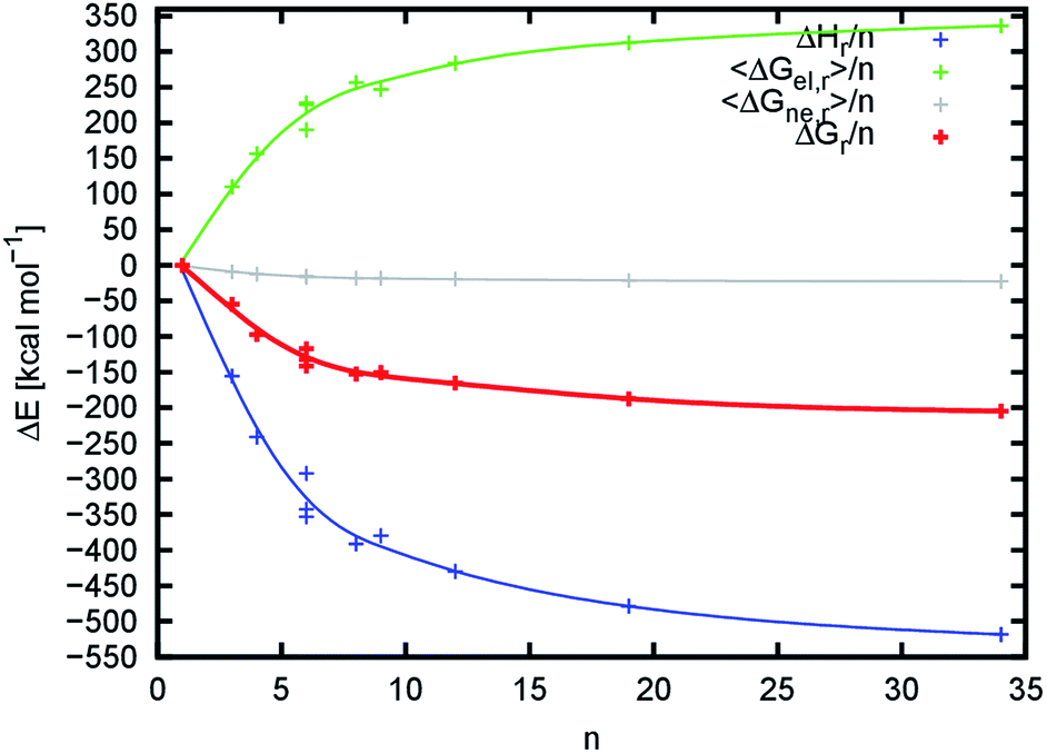Fig. 8 Dependence of change in reaction enthalpy ΔH_r, electrostatic ΔG_el,r and non-electrostatic ΔG_ne,r contributions to solvation free reaction energies and total free reaction energy ΔG_r per single chitin chain on the number of chitin chains n (excluding the entropy contributions). Lines are meant to only highlight the progress of individual energy contributions.

While the interaction between chitin chains is strongly favorable towards the assembly of chitin nanofibrils (negative enthalpy) we found that the solvent destabilizes their mutual binding. This is caused by the relatively strong interaction between nanofibrils and solvent molecules, and the fact that the contact of individual disassembled chitin chains with the solvent is higher than in an assembled nanofibril. The contribution of the solvent to the binding is expressed by the value of 〈ΔG_sol,r〉/n. The value of 〈ΔG_sol,r〉/n, which is the sum of 〈ΔG_el,r〉/n and 〈ΔG_ne,r〉/n, increases up to the limiting value (Table S8,†Fig. 8), which we estimated to be about 394.7 ± 34.7 kcal mol⁻¹. This value is smaller than the limiting value for the reaction enthalpy in the gas phase, confirming that the destabilization by the solvent is weaker than the mutual interaction between chitin chains.

The change in total reaction free energy per chitin chain is provided in Fig. 8. Its extrapolated limiting value is about −256.6 ± 24.2 kcal mol⁻¹. The initial very steep change in the total binding energy reaches an energy plateau with a very slow energy decay towards the limiting energy starting from approximately 20 chains (n = 20). From this perspective, the 676 and 8998 nanofibrils reached dimensions at which the binding enthalpy and desolvation energies are already maximized. From the enthalpy point of view, this means that the shape of the nanofibril and formed internal interaction network reached a situation very close to the crystalline chitin. From a desolvation point of view, as the number of chitin chains increases, the total surface of chitin chains that lose contact with the solvent (the proportion of the chitin chains that are desolvated upon binding) becomes predominant compared to the nanofibril surface (the proportion of the chitin chains that remain solvated). The value of 〈ΔG_sol,r〉/n must then converge to the opposite value of the solvation energy of a single chitin chain. Indeed, the value of 〈ΔG_sol,r〉/n converges to 394.7 ± 34.7 kcal mol⁻¹ while the solvation energy of the 1000 model is −399.1 kcal mol⁻¹.

The beginning of the energy plateau coincides with the size of the nanofibrils occurring in the natural chitin nanocomposites, which usually consist of 18–25 chitin molecules.⁶ It can be assumed that the evolution of chitin nanofibrils with this geometry was at least partially driven by the fact that they are the smallest nanofibrils with crystalline chitin-like properties, which combine small size for structural versatility with excellent chemical and mechanical properties.

We also use our data to predict changes in reaction entropy. Due to the length of the trajectories, we only obtained qualitative data on the simplified coarse-grained models of the simulated systems (Table S9 and Fig. S15†). The obtained data show a decrease in translational, rotational and vibrational contributions to the total reaction entropy per single chitin chain (ΔS_r/n) with an increasing number of chains, which could be expected as the structures become more compact and rigid. Due to coarse-graining of the analyzed trajectories, the model does not correctly account for all entropy changes, such as for example the decrease in hydroxyl group rotational entropy upon the formation of hydrogen bonds. Thus in future studies it will be necessary to employ more advanced techniques for entropy calculations, such as the two-phase thermodynamic (2PT) model.⁵⁹ Despite bottlenecks in the methodology used, entropy does not change the progress of the reaction free energy discussed above. The entropy converges towards about −275 cal mol⁻¹ K⁻¹, (a very crude estimate due to the irregular progress of entropy), which corresponds to a free energy contribution of about +82.5 kcal mol⁻¹. This, together with the reaction free energy can be used to predict the total contribution to binding per single unit of chitin chain (e.g. N-acetylglucosamine), which is about −8.7 kcal mol⁻¹. Since this value is in very good agreement with typical binding energies including saccharide moieties,⁶⁰ our methodology is suitable for providing consistent predictions of binding energies and affinities at least at a qualitative level.

Conclusions

Employing a theoretical approach, we elucidate the structure, dynamics, energy characteristics and aspects of self-assembly of a single chitin chain and 10 chitin nanofibrils composed of an increasing number of molecules in an aqueous environment. The molecular dynamics simulations of the smallest nanofibril model, which includes three chitin chains, indicate that nanofibril formation is driven by a variety of weak non-specific hydrogen bonds during the early stages of nanofibril formation. These non-specific hydrogen bonds, which are formed especially by the O6–H2N and O2N–H3O atom pairs, do not normally appear in crystalline chitin or assembled nanofibrils. We can speculate that their presence might be important for the efficiency of nanofibril self-assembly. Simulations of the other nine nanofibrils show relatively stable structures. The most significant discovery is axial chirality, which is exhibited by all nanofibrils. The similar behavior was already described for cellulose nanofibrils^55,56 but it seems that the molecular origin of this phenomenon in these two crystalline polysaccharides might be different. The largest axial distortion was observed for the 2220 and 6000 nanofibril systems, where the twist along the axis of the 20 unit long chains is nearly 240 and 180 degrees, respectively. This axial chirality is a consequence of the intrinsic axial chirality of single chitin chains, which is altered by interactions between chains. The stacking of chains on top of each other in the a direction preserves their axial chirality, while the presence of additional nanofibrils in the b direction significantly decreases chirality. This can be explained by dipole–dipole interactions between the acetamide groups from adjacent stacked chitin layers. These alter the mutual orientation of adjacent sugar rings along glycosidic bonds and thus influence the overall axial chirality. Essential dynamics analysis revealed that axial twist distortion is the softest dynamic mode. This might be important for the formation of protein-coated chitin nanofibrils in living organisms, where it could play a role in the binding of proteins. The calculated binding free energies reveal that the major driving force for binding is enthalpy, which is suppressed by desolvation and entropy. The progress of the total free reaction energy per single chitin chain reaches an energy plateau at about 20 chitin chains and above. This indicates that the 6760 and 8998 chitin nanofibrils exhibit binding interactions that resemble those in crystalline chitin. The resulting excellent mechanical properties together with the rather high flexibility of nanofibrils in the a and b directions may very well be one reason why evolution favored chitin nanofibrils with this geometry as basic components for biocomposites such as the exoskeleton of Arthropoda.

Acknowledgements

This research was financially supported by the Ministry of Education, Youth and Sports of the Czech Republic under the project CEITEC 2020 (LQ1601) and the project CZ.1.05/1.1.00/02.0068 financed from the European Regional Development Fund. The computational resources were provided by the CESNET LM2015042 and the CERIT Scientific Cloud LM2015085, provided under the programme "Projects of Large Research, Development, and Innovations Infrastructures". This work was also supported by the IT4Innovations Centre of Excellence project (CZ.1.05/1.1.00/02.0070, individual projects IT4I-9-11, OPEN-4-2, OPEN-5-10, OPEN-6-10 and OPEN-6-23), funded by the European Regional Development Fund and the national budget of the Czech Republic via the Research and Development for Innovations Operational Program, and the Ministry of Education, Youth and Sports of the Czech Republic via the programme "Projects of Large Research, Development, and Innovations Infrastructures" (LM2011033). The parts of this study that were conducted at the Max-Planck-Institut für Eisenforschung, Düsseldorf, Germany benefitted from financial support from the German Research Foundation (DFG) within the priority programme SPP 1420. M. F. acknowledges financial support from the Academy of Sciences of the Czech Republic through the Fellowship of Jan Evangelista Purkynĕ. Z. S. is grateful for financial support from the Max Planck Society during her stay at the Max Planck Institute for Iron Research in Düsseldorf, Germany.

Notes and references

1. Y. Wang, J. Wohlert, M. Bergenstrahle-Wohlert, Y. Tu and H. Agren, RSC Adv., 2015, 5, 54580–54588.
2. M. N. Ravi Kumar, React. Funct. Polym., 2000, 46, 1–27.
3. A. Neville, D. Parry and J. Woodheadgalloway, J. Cell Sci., 1976, 21, 73–82.
4. K. J. Kramer and D. Koga, Insect Biochem., 1986, 16, 851–877.
5. Y. Fan, T. Saito and A. Isogai, Biomacromolecules, 2008, 9, 1919–1923.
6. A. Neville, D. Parry and J. Woodhead-Galloway, J. Cell Sci., 1976, 21, 73–82.
7. D. Carlstrom, J. Biophys. Biochem. Cytol., 1957, 3, 669–683.
8. R. Minke and J. Blackwell, J. Mol. Biol., 1978, 120, 167–181.
9. J. E. Rebers and L. M. Riddiford, J. Mol. Biol., 1988, 203, 411–423.
10. M. Behr and M. Hoch, FEBS Lett., 2005, 579, 6827–6833.
11. G. Fraenkel and K. M. Rudall, Proc. R. Soc. London, Ser. B, 1947, 134, 111–143.
12. P. Sikorski, R. Hori and M. Wada, Biomacromolecules, 2009, 10, 1100–1105.
13. M. Petrov, L. Lymperakis, M. Friák and J. Neugebauer, Biopolymers, 2013, 99, 22–34.
14. S. Nikolov, M. Petrov, L. Lymperakis, M. Friak, C. Sachs, H.-O. Fabritius, D. Raabe and J. Neugebauer, Adv. Mater., 2010, 22, 519–526.
15. S. Nikolov, H. Fabritius, M. Petrov, M. Friak, L. Lymperakis, C. Sachs, D. Raabe and J. Neugebauer, J. Mech. Behav. Biomed. Mater., 2011, 4, 129–145.
16. B. Moussian, Insect Biochem. Mol. Biol., 2010, 40, 363–375.
17. H. Merzendorfer, J. Comp. Physiol., B, 2006, 176, 1–15.
18. Y. Arakane, S. Muthukrishnan, K. J. Kramer, C. A. Specht, Y. Tomoyasu, M. D. Lorenzen, M. Kanost and R. W. Beeman, Insect Mol. Biol., 2005, 14, 453–463.
19. M. E. Gagou, M. Kapsetaki, A. Turberg and D. Kafetzopoulos, Insect Biochem. Mol. Biol., 2002, 32, 141–146.
20. B. Moussian, H. Schwarz, S. Bartoszewski and C. Nüsslein-Volhard, J. Morphol., 2005, 264, 117–130.
21. Y. Arakane, C. A. Specht, K. J. Kramer, S. Muthukrishnan and R. W. Beeman, Insect Biochem. Mol. Biol., 2008, 38, 959–962.
22. H.-O. Fabritius, C. Sachs, P. R. Triguero and D. Raabe, Adv. Mater., 2009, 21, 391–400.
23. G. T. Beckham and M. F. Crowley, J. Phys. Chem. B, 2011, 115, 4516–4522.
24. E. F. Franca, R. D. Lins, L. C. G. Freitas and T. P. Straatsma, J. Chem. Theory Comput., 2008, 4, 2141–2149.
25. V. E. Yudin, I. P. Dobrovolskaya, I. M. Neelov, E. N. Dresvyanina, P. V. Popryadukhin, E. M. Ivan'kova, V. Y. Elokhovskii, I. A. Kasatkin, B. M. Okrugin and P. Morganti, Carbohydr. Polym., 2014, 108, 176–182.
26. G. T. Beckham and M. F. Crowley, J. Phys. Chem. B, 2011, 115, 4516–4522.
27. Z. Yu and D. Lau, J. Mater. Sci., 2015, 50, 7149–7157.
28. Z. Yu and D. Lau, J. Mol. Model., 2015, 21, 128.
29. E. Atkins, J. Biosci., 1985, 8, 375–387.
30. J. F. V. Vincent and U. G. K. Wegst, Arthropod Struct. Dev., 2004, 33, 187–199.
31. D. Case, T. Darden, T. Cheatham, C. Simmerling, J. Wang, R. Duke, R. Luo, R. Walker, W. Zhang, K. Merz, B. Roberts, S. Hayik, A. Roitberg, G. Seabra, J. Swails, A. Goetz, I. Kolossváry, K. Wong, F. Paesani, J. Vanicek, R. Wolf, J. Liu, X. Wu, S. Brozell, T. Steinbrecher, H. Gohlke, Q. Cai, X. Ye, J. Wang, M. Hsieh, G. Cui, D. Roe, D. Mathews, M. Seetin, R. Salomon-Ferrer, C. Sagui, V. Babin, T. Luchko, S. Gusarov, A. Kovalenko and P. Kollman, AMBER 12, University of California, San Francisco, 2012.
32. K. N. Kirschner, A. B. Yongye, S. M. Tschampel, J. González-Outeiriño, C. R. Daniels, B. L. Foley and R. J. Woods, J. Comput. Chem., 2008, 29, 622–655.
33. W. L. Jorgensen, J. Chandrasekhar, J. D. Madura, R. W. Impey and M. L. Klein, J. Chem. Phys., 1983, 79, 926–935.
34. T. Darden, D. York and L. Pedersen, J. Chem. Phys., 1993, 98, 10089–10092.
35. R. Salomon-Ferrer, A. W. Götz, D. Poole, S. Le Grand and R. C. Walker, J. Chem. Theory Comput., 2013, 9, 3878–3888.
36. D. R. Roe and T. E. Cheatham, J. Chem. Theory Comput., 2013, 9, 3084–3095.
37. E. A. Coutsias, C. Seok and K. A. Dill, J. Comput. Chem., 2004, 25, 1849–1857.
38. E. Arunan, G. R. Desiraju, R. A. Klein, J. Sadlej, S. Scheiner, I. Alkorta, D. C. Clary, R. H. Crabtree, J. J. Dannenberg, P. Hobza, H. G. Kjaergaard, A. C. Legon, B. Mennucci and D. J. Nesbitt, Pure Appl. Chem., 2011, 83, 1637–1641.
39. D. Cremer and J. A. Pople, J. Am. Chem. Soc., 1975, 97, 1354–1358.
40. V. Tsui and D. A. Case, Biopolymers, 2001, 56, 275–291.
41. N. Homeyer and H. Gohlke, Mol. Inf., 2012, 31, 114–122.
42. B. R. Miller, T. D. McGee, J. M. Swails, N. Homeyer, H. Gohlke and A. E. Roitberg, J. Chem. Theory Comput., 2012, 8, 3314–3321.
43. R. Hermann, J. Phys. Chem., 1972, 76, 2754–2759.
44. B. Honig, K. Sharp and A. Yang, J. Phys. Chem., 1993, 97, 1101–1109.
45. A. Amadei, A. Linssen and H. Berendsen, Proteins: Struct., Funct., Genet., 1993, 17, 412–425.
46. D. M. F. VanAalten, B. L. DeGroot, J. B. C. Findlay, H. J. C. Berendsen and A. Amadei, J. Comput. Chem., 1997, 18, 169–181.
47. J. Schlitter, Chem. Phys. Lett., 1993, 215, 617–621.
48. H. Schafer, A. E. Mark and W. F. van Gunsteren, J. Chem. Phys., 2000, 113, 7809–7817.
49. The PyMOL Molecular Graphics System, Version 1.6.1, Schrödinger, LLC.
50. W. Humphrey, A. Dalke and K. Schulten, J. Mol. Graphics, 1996, 14, 33–38.
51. S. Hild, O. Marti and A. Ziegler, J. Struct. Biol., 2008, 163, 100–108.
52. M. Petrov, L. Lymperakis, M. Friak and J. Neugebauer, Biopolymers, 2013, 99, 22–34.
53. S. Paavilainen, T. Rog and I. Vattulainen, J. Phys. Chem. B, 2011, 115, 3747–3755.
54. J. F. Matthews, G. T. Beckham, M. Bergenstrahle-Wohlert, J. W. Brady, M. E. Himmel and M. F. Crowley, J. Chem. Theory Comput., 2012, 8, 735–748.
55. L. Bu, M. E. Himmel and M. F. Crowley, Carbohydr. Polym., 2015, 125, 146–152.
56. K. Conley, L. Godbout, M. A. Whitehead and T. G. M. van de Ven, Carbohydr. Polym., 2016, 135, 285–299.
57. P. Sikorski, R. Hori and M. Wada, Biomacromolecules, 2009, 10, 1100–1105.
58. A. Al-Sawalmih, C. Li, S. Siegel, H. Fabritius, S. Yi, D. Raabe, P. Fratzl and O. Paris, Adv. Funct. Mater., 2008, 18, 3307–3314.
59. A. S. Gross, A. T. Bell and J.-W. Chu, Phys. Chem. Chem. Phys., 2012, 14, 8425–8430.
60. S. K. Mishra, G. Calabró, H. H. Loeffler, J. Michel and J. Koča, J. Chem. Theory Comput., 2015, 11, 3333–3345.

---

Footnote

† Electronic supplementary information (ESI) available: Tables S1–S9, Fig. S1–S15. See DOI: 10.1039/c6ra00107f

---