Preparation of spherical agglomerates from potash alum

Abstract

Salt hydrates are low-cost, readily available PCMs (phase change materials). As a core material for encapsulation the salt agglomerates can be prepared by spherical agglomeration, a well-known method to produce drug loaded microspheres in the pharmaceutical industry, but not used for PCM formulation. The two basic mechanisms in spherical crystallization are spherical agglomeration (SA) and the quasi emulsion solvent diffusion (QESD) processes. The spherical agglomerates of aluminium potassium sulfate dodecahydrate (potash alum dodecahydrate), a highly water soluble material, were produced by spherical crystallization technique in four different solvent systems. In water (good solvent)–ethanol–dichloromethane (poor solvent) ternary solvent system the agglomeration takes place by the SA mechanism. In water–ethanol–n-hexane, water–ethanol and water–isopropyl alcohol solvent systems spherical particles were produced by the QESD method. Both procedures were proved to be feasible for the preparation of spherical salt hydrate particles as core material for microencapsulation. This method gives important basis to produce phase change materials from suitable salt hydrates. The potash alum content in the spherical agglomerates was analysed by conductivity and thermogravimetric measurements and their composition by XRD. Volume weighted mean diameters (D(4,3)) of the microparticles were 66 μm, 79 μm, 89 μm, and 684 μm formed in water–ethanol–n-hexane, water–ethanol, water–isopropyl alcohol, and water–ethanol–dichloromethane solvent system, respectively. Potash alum dodecahydrate is a double salt. Due to its different solubility in the four different solvent systems it crystallized out not only as potash alum, but also in other salt forms. The enthalpy changes of spherical agglomerates produced from different solvent systems were increased proportionally with potash alum contents.

---

Introduction

Currently in particle technology the spherical form of the particles is an essential demand. Spherical agglomeration can be an applicable method to produce spherical composite particles. Kawashima and his co-workers were the pioneers, who explored the so called spherical crystallization at the end of the 80s.¹ In this process, crystallization and agglomeration were carried out simultaneously in one step. This technique has been developed for improvement of flowability and compressibility of drugs with different crystal form e.g. needle type.² The method is very effective in the enhancement of bioavailability of different pharmaceutical drugs, characterized by low water solubility and a slow dissolution profile, by improving their dissolution behaviour.

Later the method was adapted to produce microcapsules in the development of controlled release systems, since it is also applicable for co-precipitation of the drug and the encapsulating polymer in the form of a spherical particle. By involving the polymer in the anti-solvent of the drug, microencapsulation can take place,³ while by adding the polymer to the solution of the drug different spherical composite particles can be formed, such as spherical nanomatrix⁴ and spherical or hollow microspheres.^5–8 In our previous work composite CS–HSA–PSS (CS: chitosan, HSA: human serum albumin, PSS: poly(sodium-4-styrene-sulfonate)) microparticles were prepared in ethyl acetate–ethanol–water ternary solvent system by combined chemical and anti-solvent precipitation, accompanied with spherical agglomeration.⁹

Spherical agglomeration has been primarily used for improving the solubility of non-water soluble synthetic drugs.^10–12 The researchers discovered spherical agglomeration in the presence of the hydrophilic polymers enhances the solubility of the poorly soluble drug. It is supposed that the deposition of the polymer onto the crystal surface causes an increase in the wettability and thus in the solubility of the drug powder. Only a few examples of the spherical agglomeration of water-soluble drugs can be found in literature.^13–15

In the simplest way of carrying out the SA process the suspended solid particles can be agglomerated by the addition of a small amount of bridging liquid, which preferentially wets the surface of the solid. Thus surface properties of the crystals and nature of the bridging liquid play an important role in the agglomeration process.¹⁴ Chow et al. submitted some general guidelines for the spherical agglomeration of drugs based on their own experimental observations.¹³ In the case of water-soluble compounds, a water-immiscible organic solvent is used as the suspending liquid and salt solutions of high concentration without common ions can be applied as the bridging liquid. This method can be used for the agglomeration of the salt crystals after its crystallization. However, literature is lacking examples for agglomeration of highly water-soluble inorganic salts from its aqueous solution as one step procedure.

Kawashima et al. studied the SA and the QESD mechanisms in detail for the agglomeration of ascorbic acid¹⁶ and bucillamine.¹⁷ The solvent systems were composed in two different ways for the agglomeration. Using the water and ethyl-acetate solvents in miscible volume ratio for ascorbic acid, the agglomeration takes place by the QESD mechanism, but using those ones in immiscible volume ratio the agglomeration occurs by the SA mechanism. Agglomeration of the bucillamine is going on in ethanol–water solvent system by the QESD mechanism, while in ethanol–water–dichloromethane non-miscible solvent system by the SA mechanism.

It is a fact that energetics is a very important research area. Besides several research areas, the investigation of heat storage systems plays a leading role.^18,19 The possibility of the phase change materials preparation in particulate form and its microencapsulation is often explored.²⁰ According to a study of Fraunhofer Institute the price of the microencapsulated phase change materials mainly arises from the cost of the pure PCM core materials besides the charge of the microencapsulation procedure steps.²¹

The numerous inorganic phase change materials like salt hydrates are low-cost, readily available PCMs. Salt hydrates have several advantages compared to organic PCMs such as paraffin.²² They have higher volumetric heat storage capacity, high thermal conductivity, and they are non-flammable materials.

To ensure high heat transfer surface area, the salt hydrates should be used in particulate and spherical form, encapsulated in water-insoluble polymer shell. Spherical particles have minimal surface/volume ratio, which can be uniformly covered with relatively small amount of polymer. Yet, the most easily coatable shape is the sphere. The specific heat transfer area per unit volume is generally increased by decreasing the mean diameters of spherical particles. A suitable preparation method for obtaining spherical salt particles is spherical agglomeration.

The objective was to study production of salt hydrate core particles by different type of spherical agglomeration methods and to characterize the products extensively. Potash alum dodecahydrate was chosen as a model salt hydrate because of data concerning its solubility in different organic solvents. Based on the experiences in the formation of the pharmaceutical drugs by spherical agglomeration, the preparation of spherical salt hydrate particles can be solved by this low cost method.

Materials and methods

Materials

The organic solvents, i.e. dichloromethane (DCM), hexane (Hx), ethanol (a.r., EtOH) were obtained from Scharlau. Isopropyl alcohol (purum, IPA) and aluminium potassium sulphate dodecahydrate (KAl(SO₄)₂·12H₂O, puriss, 98–102%, potash alum dodecahydrate, henceforth named also as ‘reference’) was purchased from Renal and Molar Chemicals Ltd. (Hungary), respectively.

Preparation of salt agglomerates

Spherical agglomerates were prepared in a closed glass reaction vessel of 100 mL inner volume and stirred by a paddle mixer. The temperature during the whole process was kept at 25 °C by a heat transfer fluid circulated in the jacket of the vessel through a Julabo thermostat. To avoid the loss of solvents a glass condenser was applied.

Precipitation of the salt agglomerates was accomplished by a quick addition of the warm (at 40 °C saturated) salt solution in one portion to the organic solvent mixture. The saturated salt solution was prepared by dissolving 3.87 g reference salt in 14.67 g distilled water. This solution was then thermostated at 40 °C for a few hours. Given volume of this salt solution was added to the organic solvents mixtures with different compositions at 25 °C. Table 1 shows the different compositions of the starting organic solvent mixture and the added amounts of the saturated salt solutions. The formed suspension was stirred for 20 minutes at 500 rpm. Particles were filtered by a 3 μm cut-off filter paper (Macherey-Nagel 640 d) or fritted glass funnels (G4) with vacuum filtration for the further analysis.

Table 1 Preparation conditions of the precipitation processes

Sample	Volume of salt solution, mL	Volume of EtOH, mL	Volume of Hx, mL	Volume of DCM, mL	Volume of IPA, mL
Sample 1	4.8	19.5	0.00	31.5	0.00
Sample 2	6.0	54.6	22.8	0.00	0.00
Sample 3	4.0	36.0	0.00	0.00	0.00
Sample 4	2.5	0.00	0.00	0.00	47.5

---

Size analysis and morphology

The size distribution of the obtained spherical agglomerates was determined by Mastersizer 2000 (Malvern Instruments, Malvern, UK) operated by laser diffraction method. The particles were characterized by the volume mean diameter. Size measurements were carried out in suspension after the samples of dry agglomerates were re-suspended in ethanol (the stability of agglomerates against disintegration in the suspension was evaluated by observing the change of size distribution under stirring at 2000 rpm in the suspension after 5–10 min). Mie's theory, refractive index of 1.456 and absorption of 0 were used in the calculations.²³ The shape of the agglomerates was observed under an optical microscope attached to a camera. The surface morphology of the agglomerates was examined by Philips XL30 ESEM scanning electron microscope. The crystals were sputter coated with gold before scanning. The photomicrographs were taken at 25.0 kV and magnification at 100×, 1000× and 3000×.

Determination of hydrate water content by conductivity measurements

The salt content in the salt agglomerates was investigated in a 150 mL double-jacketed baker which was connected to a thermostat. In 100 g distilled water 13–20 mg salt agglomerates were dissolved. The temperature was kept at 25 °C, the solution was stirred with magnetic bar by 500 rpm. The conductivity was measured with a Radelkis OK097P electrode connected to a Radelkis OK-114 conductometer equipped with a digital multimeter. The measured digital signals were transmitted to a PC. Calibration curve between salt concentration and conductivity was calculated based on the measurements of the conductivity of KAl(SO₄)₂ in a concentration range between 0.01–0.12 g L⁻¹. Based on the fitted equation, the salt content in weight percentage in the agglomerates could be calculated.

From the concentration data, the salt (S%) and water content (W%) of the agglomerates were calculated by the eqn (1) and (2), respectively:

S% = y/(m × 10) (1)

W% = 100 − S%, (2)

where m is the mass of the agglomerated sample (g) in 100 g distilled water, y is the concentration of the salt solution (g L⁻¹), S% is the salt content and W% is the water content in w/w% of the salt agglomerates. Five and three parallel measurements were made for the reference and the samples, respectively.

Thermal properties of the agglomerates

Thermogravimetric analyses were carried out in a MOM Derivatograph Q-1500D under static air atmosphere and dynamic heating conditions (10 °C min⁻¹ heating rate) in the range of temperature from 30 to 1000 °C, applying high-grade corundum as reference. Corundum crucibles were used for the experiments.

DSC measurements

The measurements were carried out on a Setaram LabsysEvo DSC thermal analyzer, in flowing high purity nitrogen atmosphere (flow rate 50 mL min⁻¹), with a constant heating rate of 5 °C min⁻¹, using standard 100 μL aluminium crucibles. The measurements were carried out in the temperature range 30–300 °C, and the reference crucible was empty.

XRD analysis

The X-ray diffraction (XRD) analyses were carried out by a Philips PW 3710 type diffractometer equipped with a PW 3020 vertical goniometer and curved graphite diffracted beam monochromator. The radiation applied was CuKα from a broad-focus Cu tube, operating at 50 kV and 40 mA. The samples were measured in continuous scan mode with 0.02° s⁻¹ scanning speed. Data collection and evaluation was performed with X'Pert Data Collector software. X'Pert Highscore Plus software was applied for identification and for the determination of the microstructures. The mean crystallite sizes were calculated using Scherrer's relationship,

L = K·λ/(B·cos θ), (3)

where L is the mean crystallite size in Angstrom, K is the shape factor equals 0.9, B is the broadening of the diffraction line measured at the half of its maximum intensity in radians, λ is the wavelength of the X-rays and θ is the Bragg's diffraction angle.

Results and discussion

Solvents selection for the agglomeration systems

In the literature there is a lack of the spherical crystallization of water-soluble salts from its aqueous solution by precipitation and agglomeration in one step. The selection of the solvent system for the agglomeration was based on the miscibility of solvents and the solubility of salt in individual solvents. Three kinds of solvents are needed: a good solvent – which dissolves the material to be agglomerated – and it should be miscible with a bad or poor solvent, i.e. with anti-solvent. The latter induces the precipitation or crystallization of the solute. The third auxiliary material is a bridging liquid, which shows good adhesion (or wetting) to crystals and forms liquid bridges between them during the process.

The precipitation of water-soluble salts generally takes place from their aqueous solution by adding different alcohols or acetone. The solubility of the model salt hydrate was examined in different alcohol–water (e.g. ethanol–water) systems by Mullin et al.²⁴ and Mydlarz et al.²⁵ as well. Utilizing their experiences, ethanol was used as poor solvent in our experiments. In previous work⁹ to produce spherical agglomerates of water soluble polymer, a ternary solvent system was used. For potash alum the equilibrium phase data are known for ethanol–water–dichloromethane²⁶ and ethanol–water–hexane²⁷ systems that were used as basic data for the ternary solvent system. The dichloromethane and the hexane act also as bad solvents, and thus, as a medium they can cause the flocculation of the salt crystals to reduce its surface or can help to form the required composition for the quasi emulsion. On the basis of the ternary solvent mixture experiments various alcohol–water mixtures were tested in order to simplify the solvent composition.

Preparation of the agglomerates by SA mechanism

Sample 1 (S1) was prepared in water–dichloromethane–ethanol ternary solvent system. The equilibrium solubility (indicated by ●) and the tie line data (indicated by ■) of the applied solvent system were published by Merzoungui and his co-authors,²⁶ and phase diagram (Fig. 1a) was drawn based on these data. Tie lines are the lines that connect two phases which are in equilibrium on a ternary phase diagram.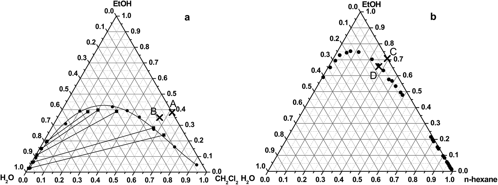

Fig. 1 Studied spherical agglomeration processes on the ternary phase diagram of the water–ethanol–dichloromethane (a)²⁶ and water–ethanol–hexane system (b).²⁷

The initial composition of the organic solvent mixture was the following: dichloromethane: 61.8% (v/v), ethanol: 38.2% (v/v) (denoted by A on Fig. 1a). After addition of the aqueous salt solution the final ratio of the solvent was 56.5% (v/v) of dichloromethane, 34.9% (v/v) of ethanol, and 8.6% (v/v) of water (point B on Fig. 1a.). The change of the composition of the solvent mixture can be represented by an arrow, which starts from the cross, located on the side of the triangle and moves to the direction to the water vertex of the triangle. The final mixture composition is situated in the miscible region in the ternary phase diagram.

The salt agglomerates were precipitated due to the high initial supersaturation induced by the rapid reduction of the solubility of the salt after adding the salt solution in one portion (‘one-shot’) to the organic solvent mixture. The decrease in solubility was achieved by the anti-solvent effect of the organic solvents and the cooling of the 40 °C saturated aqueous salt solution down to 25 °C.

Under the preparation conditions the interaction between water and ethanol was stronger than the interaction between the salt and water. It means that the main part of the introduced water dissolved in the solvent mixture, leaving the salt in less hydrated state. Due to the decreased water content in the formed droplets and the very low solubility of the salt in the organic solvent mixture, the salt precipitates immediately. Because of the bad wettability of the precipitated salt crystals with the solvent medium (dichloromethane), they formed spherical agglomerates with the non-precipitated, though saturated salt solution serving as binding liquid.

Preparation of the agglomerates by QESD mechanism

The spherical agglomeration was carried out in both of the ternary and the binary solvent systems by QESD mechanism. Sample 2 (S2) was prepared in the water–n-hexane–ethanol ternary solvent system. The liquid–liquid equilibrium data (indicated by ●) of the applied solvent system (Fig. 1b) was published by Moriyoshi et al.²⁷

The initial composition of the organic solvent mixture (Hx: 29.5%, EtOH: 70.5%) and the final solvent concentrations of the mixture (Hx: 27.3%, EtOH: 65.5%, H₂O: 7.2%) after addition of the aqueous salt solution can be seen in the ternary diagram showed by point C and D, respectively. The final mixture composition is situated in the miscible region in the ternary phase diagram.

In this case the interaction between the water and the salt was higher than the interaction between the n-hexane and the water, which led to the formation of quasi emulsion droplets. The crystallization took place inside the droplets, resulted in almost perfectly spherical crystal agglomerates.

Preliminary experiments showed that in a water–ethanol mixture at 50% (v/v) ethanol concentration potash alum crystallized in the regular potash alum dodecahydrate form, but at 90% (v/v) ethanol concentration the dodecahydrate form was replaced by perfect spheres. Sample 3 (S3) and sample 4 (S4) were prepared in water–ethanol and water–isopropyl-alcohol solvent systems, respectively. The solubility of the potash alum dodecahydrate in these water–alcohol solvent systems is very similar at 26.302% (m/m) alcohol concentration 0.573 g and at 24.140% (m/m) 0.771 g salt hydrate/100 g solution at 25 °C for ethanol and isopropyl alcohol, respectively.²⁵ The solubility decreases to a sufficiently low level at the 90% ethanol and 95% isopropyl alcohol concentrations, at the generated high supersaturation the nucleation rate is so high, that there is enough time to be complete the solidification before the water could mix with alcohols.²⁸ This precipitation also resulted in almost perfect spheres like in the above water–n-hexane–ethanol solvent system.

Size, and morphology

As shown in Fig. 2, the type of agglomeration method had a great effect on the size of particles. Applying the SA method the size of spherical agglomerates was much larger (S1, volume-weighted mean D(4,3) = 684 μm) and had a wider size distribution than using the ESD method (volume-weighted mean D(4,3) = 66 μm, 79 μm and 89 μm for S2, S3, and S4, respectively). It can also be observed that neither of the samples had monomodal distribution, since each obtained size distribution contained another little peak in the region below 20 μm and 200 μm for sample 2–4 and sample 1, respectively; however, less than 10% of each sample fell into these smaller size ranges. The size distribution measurement the sample 1 showed high level of disintegration, while the other samples were quite stable, the negligible decrease of average volume diameters came from the disaggregation of agglomerates formed as a result of drying. The particle size distribution did not show significant change with stirring rate, after sufficient dispergation of particles in ethanol.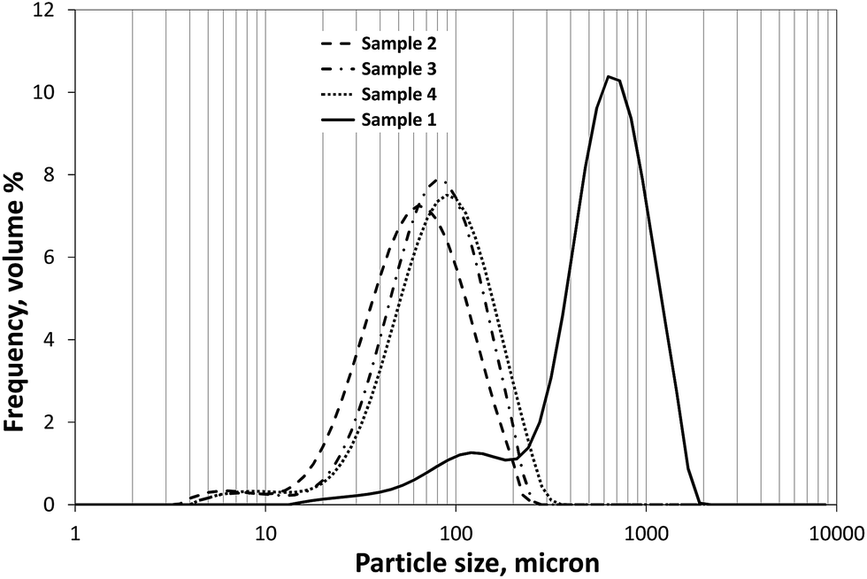

Fig. 2 Typical particle size distributions of the samples produced by various crystallization solvent systems. S1 (solid line), S2 (dashed line), S3 (dash-dot line), S4 (dotted line).

Scanning electron micrographs (Fig. 3a and b) showed that the agglomerates prepared by SA method (S1) are built up from lots of little octahedrons and these crystals were self-organized along the crystal edges. Based on the crystal structure these agglomerates were assumed to be potash alum dodecahydrate.²³

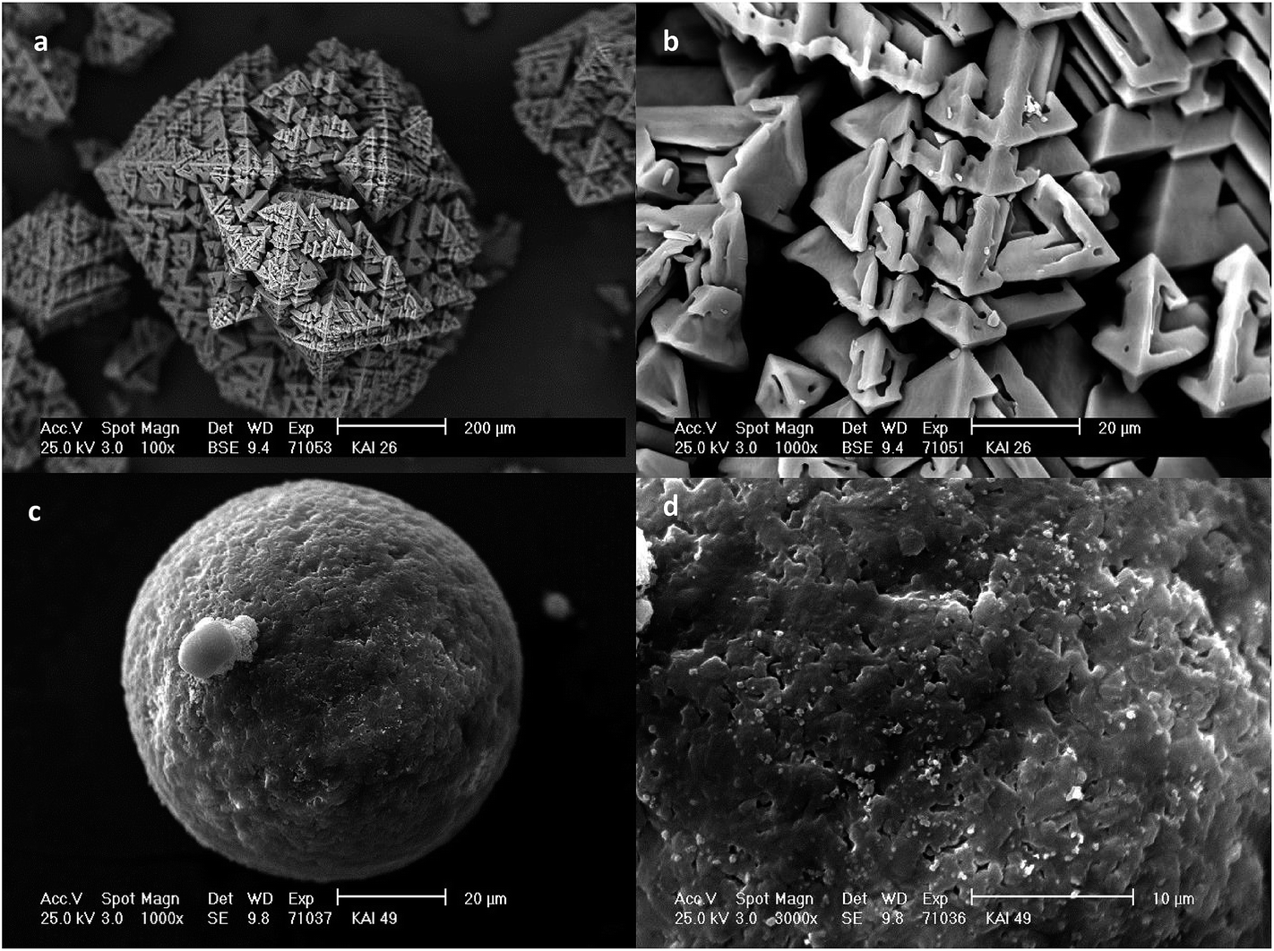Fig. 3 Typical SEM pictures of agglomerates obtained by SA (a and b) (S1) and QESD (c and d) (S2) method.

Scanning electron microscopy also confirmed that using ESD method (S2) almost spherical potash alum particles could be prepared with smooth surface (Fig. 3c and d).

Water content in the agglomerated samples from conductivity measurements

The water content of the agglomerated samples can be estimated with a relatively simple and quick method by measuring the conductivity of the samples. On the basis of the conductivity measurement in a concentration range between 0.01–0.12 g L⁻¹ of KAl(SO₄)₂ calibration curve was calculated (see eqn (3)) using the reference. The concentration of KAl(SO₄)₂ of the sample solutions vs. conductivity data resulted in a curve described as a quadratic equation (eqn (3)). The obtained equation is the following (R² = 0.999):

y = 7.6362 × 10⁻⁰⁷·x² + 4.1445 × 10⁻⁰⁴·x − 9.7531 × 10⁻⁰⁴ (4)

, where y is the concentration of the salt solution (g L⁻¹), x is the conductivity (μS cm⁻¹).

The water content (W%) of the S1–S4 were calculating using eqn (1) and (2). The obtained data are summarized in Table 2. The theoretical water content in potash alum dodecahydrate is 45.53%. The water content of reference and S1 are slightly higher than the theoretical (by 3.2% and 5.3%, respectively). For the sample 2–4 significant differences could be noticed in a negative direction concerning the water content. The conductivity measurements suggested that S1 could be identified as potash alum dodecahydrate. The other three samples were expected as not pure potash alum dodecahydrate. To prove these assumptions thermogravimetric and XRD analyses were carried out.

Table 2 Calculated water mass fraction and calculated average water of hydration content (n_w) of the agglomerated samples (S1–S4) from the conductivity measurements (W%) and TG curves (TG%)

Sample	W%, w/w%	TG% (50–300 °C)	n w
Reference	46.98%	46%	12.2
S1	47.96%	46.13%	12.3
S4	44.71%	39.02%	9.2
S2	37.82%	33.59%	7.3
S3	38.79%	31.77%	6.7

---

Thermogravimetric analysis

According to the literature^29,30 the potash alum dodecahydrate loses its water of hydration until 300 °C in three steps. The products of these steps cannot be distinctly identified. The reference potash alum dodecahydrate lost its water of hydration in three steps as described in the literature^29,30 (see Fig. 4). According our to TG curve the reference sample lost about 9.3 molecules of water in two steps between 30 and 210 °C (9.3 mol H₂O/1 mol KAl(SO₄)₂), and the rest eliminated in the third step around 250 °C. A similar phenomenon was observed in the case of dehydration of sample 1. Sample 1 crystallized in dodecahydrate form similar to the reference sample. Kishimura et al.³¹ showed that the peak of the dehydrated KAl(SO₄)₂ appeared at 180 °C in XRD spectrum, whilst at 250 °C the spectrum was identical with the spectrum of pure crystalline anhydrous KAl(SO₄)₂. It means the hydrated KAl(SO₄)₂ lost the crystallization water partially. For the reference at 250 °C the water loss in percentage is 45.5% in agreement with the theoretical water content of KAl(SO₄)₂·12H₂O. Analysing the TG curves of the sample 4, 2, and 3 it can be stated that the water contents (TG%) decreased in the given order (see also Table 2). The samples showed significant differences in the weight loss percentages around the melting point temperature, that is 92–93 °C. The average number of water of hydration molecule of the samples (n_w) which corresponds to the weight loss during the heat treatment can be seen in Table 2.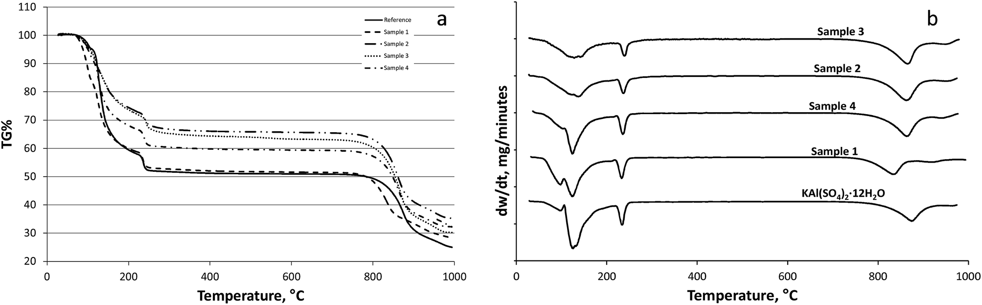

Fig. 4 Derivatograms (TG (a) and DTG (b)) for the dehydration of the reference material and the samples (S1–S4) crystallized from different solvent systems. Reference (solid line), S1 (dashed line), S2 (dash-dot-dot), S3 (dotted line), S4 (dash-dot line).

The difference from the dodecahydrate form suggests that the agglomerated samples (except sample 1) are not pure potash alum dodecahydrate, hence for the determination of composition of the other agglomerated samples XRD analysis was carried out.

XRD analysis

According to the scanning electron microscope, the thermogravimetric measurements and XRD analysis sample 1 was clearly identified as potash alum dodecahydrate. Fig. 5 shows the XRD patterns of the reference and four different agglomerated samples: the peak intensities of the reference sample and the sample 1 were notably higher than the samples prepared in the three solvent systems (S2–S4) indicating that these salt hydrate agglomerates have partially amorphous structure and have different degree of crystallinity.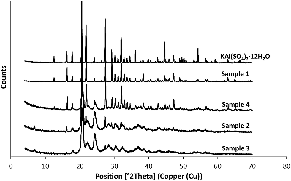

Fig. 5 XRD patterns of the reference materials and the samples (S2–S4) prepared by QESD method.

On the basis of the XRD pattern besides the potash alum these samples contain further four different salts such as rostite (Al(SO₄)(OH)·5H₂O), alunogen (Al₂(SO₄)₃·17H₂O), anhydrous KAl(SO₄)₂ and K₂SO₄. An evaluation of the results of the X-ray diffraction studies showed, that in the crystalline phase all the three samples contained the five different salts but in different ratios. Table 3 shows the approximate calculation of the mass fractions of the different components in these agglomerated samples.

Table 3 Calculated mass fraction of the different components in the agglomerated samples (S2–S4)

Components	S2	S3	S4
	Mass fractions, %
KAl(SO4)2·12H2O	74	59	74
Al(SO4)(OH)·5H2O	13	26	9
KAl(SO4)2	4	5	10
K2SO4	7	5	5
Al2(SO4)3·17H2O	3	6	2

---

Line broadening of the peaks can also be noticed in the case of the samples 2–4. This line broadening indicates the differences of the microstructures of the different crystalline phases. To describe these microstructures on the basis of the famous Scherrer equation³² the mean crystallite (coherently scattering domain) sizes were calculated for the different crystalline phases. The calculated data are shown in the Table 4.

Table 4 Calculated crystallite sizes of the different crystalline phases in the samples 2–4

Sample	Considered line of potash alum: 5.45 Å (210)	Considered line of rostite: 4.26 Å (220)	Considered line of alunogen: 3.97 Å (1–31)	Considered line of KAl(SO4)2: 3.63 Å (011)	Considered line of (K2SO4): 3.17 Å (102)
Mean crystallite size, Å
S2	3489	530	69	124	83
S3		441	63	121	41
S4	2360	505	66	136	133

---

DSC analysis

During the heating of salt hydrate samples both the melting enthalpy and the heat of hydration water elimination are present in the DSC curve.

Analysing the relationship between the water of hydration content of the samples and the measured heat (heat effect), a linear correlation can be observed. Using the water of hydration content data from Table 2 for the calculation of a ratio between the water content of the samples and the reference, a proportionality factor can be calculated (Table 5). By the aid of this proportionality factor, expected heat can be estimated for the samples. The correlation of the measured and the calculated sample heats are quite good. At the DSC measurements, the sample amount is much lower and the heating rate is much slower than at the TG measurements. These differences in the measurement conditions can cause the deviation of the calculated heats from the measured.

Table 5 Measured heat values concerning to the eliminated water of hydration on the basis of the DSC curves

Samples	Heat, J g^−1	Sample heat to reference heat, %	Water of hydration proportionality to the reference	Calculated sample heat from water of hydration ratio, J g^−1
Reference (48–260 °C)	999.6
S1 (44–235 °C)	947.8	95%	1.0049	1004.5
S4 (42–280 °C)	727.3	73%	0.7522	752.0
S2 (41–215 °C)	522.7	52%	0.5969	596.7
S3 (44–215 °C)	478.4	48%	0.5478	547.6

---

Investigating the correlation between the measured heat and the potash alum dodecahydrate content of the samples, simple proportionality can be observed. The calculated ratio of the measured heat of the reference and that of the samples 1–4 (Table 5) shows that the enthalpy changes of spherical agglomerates produced from different solvent systems were increased proportionally with potash alum dodecahydrate contents (compare with the data in Table 3). In case of the sample 4 the difference between the calculated heat ratio and the potash alum percentage from the XRD analysis is negligible. For sample 3 this difference is a little bit higher and for sample 2 it is the highest. The possible reason of these variations is that from these XRD measurements the crystalline and the amorphous phase ratio cannot be established quantitatively, therefore, the extent of changes in the absorbed heat caused by the presence of amorphous phase cannot be calculated either. Although it can be stated that the sample 4 showed an almost totally crystalline structure, while the sample 2 represented a slightly noisy XRD curve which denotes the sign of some amorphous phase.

Conclusions

Spherical agglomerates of salt hydrate were prepared successfully both by spherical agglomeration and by quasi emulsion methods. Agglomerates produced by SA method are crystallized in dodecahydrate form, but less stable and less spherical than the others. Agglomerates produced by QESD method are more stable and almost perfectly spherical, but not pure potash alum dodecahydrate, however they contain further four different crystal salts besides potash alum dodecahydrate.

Spherical crystallization was verified to be a feasible method for the production of agglomerates of suitable salt hydrates that are intended to use as PCM core material in microencapsulation. For the successful preparation of the spherical agglomerates, the composition of the solvent mixture has to ensure a very high generated supersaturation, i.e. very low solubility of the salt hydrate in the bad solvent and the nucleation rate need to be so high that there is enough time for the complete solidification before the water mixes with the bad solvents. Optimizing the salt hydrate solubility in the solvent mixture salt hydrate agglomerates can be prepared with sufficiently high enthalpy to use these agglomerates as cores of encapsulated PCM materials.

According to DSC measurements the enthalpy changes of spherical agglomerates produced from different solvent systems were increased proportionally with potash alum dodecahydrate and average water of hydration contents confirmed by XRD and TG analysis.

Symbols, indices

CS	Chitosan
HSA	Human serum albumin
PSS	Poly(sodium-4-styrene-sulfonate)
DCM	Dichloromethane
EtOH	Ethanol
H2O	Water
IPA	Isopropyl alcohol
TG%	Water content of the agglomerated samples from the TG measurements
S%	The salt content in w/w% of the salt agglomerates
W%	The water content in w/w% of the salt agglomerates from the conductivity measurements
n w	Average water of hydration content in the salt agglomerates from TG measurements

Acknowledgements

The authors acknowledge the financial support of the Hungarian state and the European Union under TAMOP-4.2.2A-11/1/KONV-2012-0072.

References

1. Y. Kawashima, M. Okumura and H. Takenaka, Science, 1982, 216, 1127–1128.
2. A. N. Usha, S. Mutalik, M. S. Reddy, A. K. Ranjith, P. Kushtagi and N. Udupa, Eur. J. Pharm. Biopharm., 2008, 70, 674–683.
3. M. Ueda, Y. Nakamura, H. Makita and Y. Kawashima, J. Microencapsulation, 1993, 10(1), 25–34.
4. K. Tahara, T. Sakai, H. Yamamoto, H. Takeuchi and Y. Kawashima, Int. J. Pharm., 2008, 354(1–2), 210–216.
5. M. Yang, F. Cui, B. You, J. You, L. Wang, L. Zhang and Y. Kawashima, J. Controlled Release, 2004, 98, 219–229.
6. Y. Kawashima, T. Niwa, T. Handa, H. Takeuchi, T. Iwamoto and Y. Itoh, Chem. Pharm. Bull., 1989, 37(2), 425–429.
7. Y. Sato, Y. Kawashima, H. Takeuchi and H. Yamamoto, Eur. J. Pharm. Biopharm., 2005, 5, 297–304.
8. Y. Kawashima, T. Niwa, H. Takeuchi, T. Hino and Y. Ito, J. Controlled Release, 1991, 16(3), 279–289.
9. A. Fodor-Kardos, J. Toth and J. Gyenis, Powder Technol., 2013, 244, 16–25.
10. A. R. Tapas, P. S. Kawtikwar and D. M. Sakarkar, Int. J. Drug Delivery, 2010, 2, 304–313.
11. V. B. Yadav and A. V. Yadav, Int. J. Pharma Bio Sci., 2010, V1(1) , http://www.ijpbs.net/36.pdf, accessed January 2016.
12. M. V. Gadhave and S. K. Banerjee, Int. J. Curr. Pharmaceut. Clin. Res., 2014, 6(4), 363–369.
13. A. H. L. Chow and M. W. M. Leung, Drug Dev. Ind. Pharm., 1996, 22(4), 357–371.
14. A. Bausch and H. Leuenberger, Int. J. Pharm., 1994, 101(1–2), 63–70.
15. Y. Kawashima, F. Cui, H. Takeuchi, T. Niwa and T. Hino, Chem. Pharm. Bull., 1996, 44(4), 837–842.
16. Y. Kawashima, H. Takeuchi, H. Yamamoto and K. Kamiya, KONA, 2002, 20, 251–262.
17. K. Morishima, Y. Kawashima, Y. Kawashima, H. Takeuchi, T. Niwa and T. Hino, Powder Technol., 1993, 1(76), 57–64.
18. W. Liang, G. Zhang, H. Sun, Z. Zhu and A. Li, RSC Adv., 2013, 3, 18022.
19. Q. Tang, J. Sun, S. Yu and G. Wang, RSC Adv., 2014, 4, 36584.
20. W. Hu and X. Yu, RSC Adv., 2012, 2, 5580–5584.
21. http://cdn2.hubspot.net/hub/55819/file-30934935-pdf/docs/pcm_price_challenge.pdf, accessed August 2015.
22. A. Kardam, S. S. Narayanan, N. Bhardwaj, D. Madhwal, P. Shukla, A. Verma and V. K. Jain, RSC Adv., 2015, 5, 56541.
23. J. W. Anthony, R. A. Bideaux, K. W. Bladh and M. C. Nichols, Handbook of Mineralogy, Mineralogical Society of America, Chantilly, VA, USA, http://www.handbookofmineralogy.org/pdfs/potassiumalum.pdf, accessed August 2015, pp. 1–1110.
24. J. W. Mullin and M. Sipek, J. Chem. Eng. Data, 1981, 26, 164–165.
25. J. Mydlarz and A. G. Jones, J. Chem. Eng. Data, 1990, 35, 214–216.
26. A. Merzougui, A. Hasseine, A. Kabouche and M. Korichi, Fluid Phase Equilib., 2011, 309, 161–167.
27. T. Moriyoshi, Y. Uosaki, H. Matsuura and W. Nishimoto, J. Chem. Thermodyn., 1988, 20, 551–557.
28. A. Sano, T. Kuriki, Y. Kawashima, H. Takeuchi, T. Hino and T. Niwa, Chem. Pharm. Bull., 1990, 38(3), 733–739.
29. J. F. Dai, R. Q. Ling and K. Z. Wang, Adv. Mater. Res., 2011, 418–420, 282–285.
30. R. Wojciechowska, W. Wojciechowski and J. Kamiński, J. Therm. Anal., 1988, 33(2), 503–509.
31. H. Kishimura, Y. Imasu and H. Matsumoto, Mater. Chem. Phys., 2015, 149–150, 99–104.
32. A. le Bail, Powder Diffraction: Theory and Practice, ed. R. E. Dinnebier and S. J. L. Billinge, Royal Society of Chemistry, Cambridge, 2008, ch. 5, p. 142.

---