Smoothed particle hydrodynamics simulation of viscoelastic flows with the slip-link model
Hualong
Feng
abd,
Marat
Andreev
ac,
Ekaterina
Pilyugina
ab and
Jay D.
Schieber
*abcd
aCenter for Molecular Study of Condensed Soft Matter, 3440 S. Dearborn Street, Chicago, IL 60616, USA
bDepartment of Chemical and Biological Engineering, 10 W. 33rd Street, Chicago, Illinois 60616, USA
cDepartment of Physics, Illinois Institute of Technology, 3101 South Dearborn Street, Chicago, IL 60616, USA
dDepartment of Applied Mathematics, Illinois Institute of Technology, 10 West 32nd Street, Chicago, IL 60616, USA. E-mail: schieber@iit.edu
First published on 10th May 2016
Abstract
We demonstrate the ability to simulate complex flows of entangled polymer melts using a high-fidelity slip-link model. Given the strong connections of the underlying molecular model to an atomistic description, nearly ab initio predictions of complex processing are feasible. Moreover, the method retains sufficient information which might allow extraction of detailed polymer chain conformations imposed by the flow. The macroscopic transport equations are solved using smoothed-particle hydrodynamics consistently with the stresses calculated using stochastic simulation of an ensemble of polymer chains in each particle. The polymer model uses only a single adjustable parameter whose value is determined from equilibrium stress relaxation. All other parameters are determined from atomistic simulation. Thereafter, nonlinear rheology predictions are made without any parameter adjustment. As a demonstration, we simulate journal-bearing flow of a moderately entangled polymer. Although the flows considered here are two dimensional, the required computational resources demonstrate that three dimensional flow calculations are accessible.
Design, System, ApplicationThe performance of many advanced materials depend on molecular conformations following processing. Polymeric materials are particularly difficult to model out of equilibrium, because of the very large relaxation times that can arise, making the interplay between molecular conformations and flow nontrivial. We present here a numerical tool that allows the prediction of molecular conformations of entangled polymers during and following processing. This is the necessary first step towards molecular design of advanced soft materials. |
1 Introduction
The largest component of many advanced materials is the polymer matrix. Not surprisingly, then, the annual production of polymers is estimated to be worth over $100 billion. The final properties are dependent on both the chemical makeup of the polymer, and on individual chain conformations after processing. For example, some electrically conductive polymers exhibit a thermoelectric effect, which might be exploited for harvesting energy from waste heat and depends on the ratio of its electrical conductivity to thermal conductivity.1,2 Both the thermal conductivity3–6 and the electrical conductivity7 are determined by the final chain conformations, which in turn are determined by the rheology during processing. However, their rheological properties depend not just on processing conditions, but are also dependent on polymer chemistry. Therefore, one needs to solve several properties that vary with time and space, and are strongly coupled.By utilizing recent advances in the molecular modeling of entangled polymers, we present a tool that could be useful in the virtual design of molded polymer parts, for example. As input, our simulation tool would require the geometry of the mold, as well as inlet and outlet pressures. Knowledge of the polymeric material is also required, such as the chemical makeup of the polymer, its molecular architecture, and its molecular weight distribution, if polydisperse. The model has several molecular-architecture-independent parameters. However, we have shown that all but one of these can be found from atomistic simulations, and we have reason to believe that this final parameter might also be predicted. One could then accurately predict flow, stresses, and coarse-grained molecular conformations during flow—during injection molding, for example—without any adjustable parameters. Moreover, in theory, one could further fine grain these conformations to predict polymer chain conformations on an atomistic level for any point in the fluid. As a result, further analysis could be used to predict relevant macroscopic properties, such as optical clarity, birefringence, electrical or thermal conductivity, etc.
For the moment, we consider only isothermal flow. However, heating and cooling can also be implemented in a straightforward way, which would also require something like temperature boundary conditions. In that case, one could also simulate the structural properties upon cooling, which is important in injection molding, or additive manufacturing. In other words, final product performance could be predicted with minimal or no knowledge from experiment. Since actual processing can take minutes, and atomistic simulations access timescales of only order 1 μs, our proposed simulation tool bridges more than 10 orders of magnitude in time.
Predicting the flow of polymers and their subsequent conformations during processing is a formidable challenge. Their rheology is not described by the Navier–Stokes equation even approximately. Instead, one needs to solve the equation of motion, which represents a continuum-level momentum balance, simultaneously with a constitutive equation that relates stresses to velocity fields.8 Recently, mean-field molecular models have been developed that are able to make quantitative predictions of stresses in arbitrary homogeneous flow fields.9,10 These so-called slip-link models require only three molecular-weight-independent parameters in order to make predictions: the molecular weight of a Kuhn step MK; the entanglement activity β, which determines entanglement density; and a timescale of Kuhn step motion τK, which embodies friction.
All but the last of these parameters can be found from atomistic Monte Carlo simulations,11,12 since they depend on chain conformations only. Monte Carlo simulations can exploit non-physical chain-crossing moves to relax chain conformations much more efficiently than obtained with molecular dynamics. Once these conformations are found, Kröger's Z1 algorithm13,14 can be used to find entanglements arising from chain uncrossability—the so-called primitive path. From information about the chain end-to-end length distribution, and the primitive-path-length distribution, the slip-link model parameters are found unambiguously.
Even the last parameter might also be accessible by molecular dynamics simulations, although that has not yet been demonstrated. Moreover, these models might provide sufficient information to reconstruct detailed information about molecular conformations.15,16 These conformations in turn could be used to predict many material properties.
Slip-link models are computationally expensive, which greatly prohibited their use in predicting flows in complex geometries. However, two recent advances have greatly reduced the costs. First, a universal version of the model was found by lumping larger segments of the polymer chain together, which resulted in a speed up of more than two orders of magnitude.12,17 Secondly, the numerical algorithm was rewritten for graphical processors, which gives another 2.5 orders of magnitude decrease in cost.18 As a result, flows in complex geometries are now feasible, which we demonstrate here.
It is widely accepted that the dynamics, and hence the rheology of long-chained polymer liquids is primarily determined by entanglements, which arise from the inability of chains to cross through one another. Their importance was first postulated by Edwards,19 and the first full rheological constitutive equation based on the idea was the tube model, proposed by Doi and Edwards.20 The tube picture is used to force the chain to reptate along its backbone, while perpendicular motions are suppressed. Since then, there have been many different mathematical tube models for various deformations and various chain architectures to force the calculations to come more in line with experiments.
More recently an alternative approach to model entanglements has been used with considerable success in predicting experimental observations. In this slip-link model, the chains are restricted to move through infinitesimal rings which mimic entanglements, or uncrossability effects.21,22 In contrast to tube models, many physical effects such as reptation, or primitive-path-length fluctuations arise naturally from the model, rather than their being put into the model. Moreover, the slip-link model is applicable to any deformation and arbitrary chain architecture.12,23–26
A similar picture has been used to motivate some computer simulations with similar physics. However, in contrast to these simulations, each implementation of the slip-link model is represented by a well-defined mathematical object. Having such a mathematical description is valuable for at least two reasons. First, it is possible to examine in detail the conformity of the model to highly developed restrictions of non-equilibrium thermodynamics (GENERIC = general equation for nonequilibrium/equilibrium reversible/irreversible coupling). As a result, one can guarantee that energy is conserved, entropy is not destroyed, and that the proper stress tensor expression is being used, among other things.27 Secondly, and critically important here, alternative algorithms can be derived for numerical calculations of model predictions. This last point was crucial in developing the GPU-capable code.
In this manuscript we show that the recent advances in computation of the discrete slip-link model allow us to make flow calculations in complex geometries. Given the remarkable fidelity of the model to experimental measurements, such calculations should be very reliable for making predictions. For the complex geometries used in processing, our slip-link model requires a macroscopic simulation technique that is Lagrangian rather than Eulerian.
Recently, a combination of smoothed particle hydrodynamics (SPH) with a simple polymeric fluid model was proposed by Vázquez-Quesada et al.28 SPH was originally developed by Gingold and Monaghan29 for astrophysical problems but was recently applied successfully to other problems, including simulations of incompressible flow, viscoelastic flow, and solid mechanics.31–32 SPH became particularly popular for graphical visualization of water and other liquids, which led to development of highly efficient algorithms. The method is known to be able to handle free surfaces and moving boundaries well and proved to be robust and reliable. Vázquez-Quesada et al. showed that the SPH method follows the structure of non-equilibrium thermodynamics (it is GENERIC compliant)28,33 and successfully applied it, together with the Oldroyd-B model, to microrheology simulations.34 In other words, not only are the continuum equations thermodynamically allowed, even their spatial discretizations in SPH can be made compliant. In this paper we combine SPH with the recent DSM version for GPUs to perform non-homogeneous flow calculations for entangled polymer melts.
2 Simulation
2.1 Discrete slip-link model
The discrete slip-link model (DSM) is a single-chain, mean-field model for the dynamics of entangled polymers. In contrast to tube models, it includes explicitly stochastic fluctuations in the number of entanglements, monomer density along the primitive path, and primitive path lengths. Although it is possible to find some analytic predictions for the model,22 numerical solutions are usually required for dynamic predictions. These calculations are done most easily by stochastic simulation of an ensemble of independent trajectories, typically order 1000 chains. Here we give only a brief description of the mathematical model.The polymer chain is coarse-grained to the entanglement level, with conformation described by variable set Ω, and chain conformation distribution in equilibrium is given by peq(Ω). This equilibrium distribution is analytic and can be used to calculate observables. Additionally, it is used to generate initial configurations for the chain ensemble efficiently. The dynamics of the model is given by
 | (1) |
![[script L]](https://www.rsc.org/images/entities/char_e144.gif) [Ω; (∇v(t))] =
[Ω; (∇v(t))] = ![[script L]](https://www.rsc.org/images/entities/char_e144.gif) eq[Ω] +
eq[Ω] + ![[script L]](https://www.rsc.org/images/entities/char_e144.gif) flow[Ω; (∇v(t))], where
flow[Ω; (∇v(t))], where  is present only in flow and
 ![[script L]](https://www.rsc.org/images/entities/char_e144.gif) eq satisfies
eq satisfies0 = ![[script L]](https://www.rsc.org/images/entities/char_e144.gif) eq[Ω]peq(Ω; t), eq[Ω]peq(Ω; t), | (2) |
![[script L]](https://www.rsc.org/images/entities/char_e144.gif) eq leaves the equilibrium distribution unchanged. Here, Qi is the conformation of entangled strand i.
eq leaves the equilibrium distribution unchanged. Here, Qi is the conformation of entangled strand i. ![[script L]](https://www.rsc.org/images/entities/char_e144.gif) eq is non-trivial, and comparisons of chain statistics with analytic integrations of peq(Ω) are made to validate numerical implementation in equilibrium. Since
eq is non-trivial, and comparisons of chain statistics with analytic integrations of peq(Ω) are made to validate numerical implementation in equilibrium. Since ![[script L]](https://www.rsc.org/images/entities/char_e144.gif) flow leads to a trivial change to the code, we trust our numerical results in flow as well.
flow leads to a trivial change to the code, we trust our numerical results in flow as well.
From another point of view, we postulate two dynamic processes for the time evolution of the chain: movement of the chain itself—sliding dynamics (SD)—and the movement of the chains in the mean field—constraint dynamics (CD). These processes are made to be consistent with one another.
As mentioned above, each chain conformation is stochastically independent of every other chain in the ensemble, which makes parallelization of the code trivial, and scalability ideal. Nonetheless, the physics of the chains do interact through a dynamic mean-field treatment of CD. Namely, each entanglement may be destroyed by CD through a first-order reaction rate, whose time scale is determined by the matrix of chains. These rates are found from the rate of entanglement destruction by SD, in order to maintain self consistency.
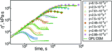
DSM has been shown to be successful in predicting both the equilibrium relaxation modulus and dielectric relaxation properties simultaneously. For example, in Fig. 1 we show data for the transient viscosity of a polyisoprene melt during inception of shear flow measured by ref. 35. The Kuhn step molecular weight MK and entanglement activity β can be found from primitive-path analysis of atomistic simulations. The frictional parameter τK is then found from the equilibrium dynamic modulus from a polyisoprene of smaller molecular weight. The predictions shown in this figure are made without parameter adjustment. Furthermore, it captures elongational flow at least up to stretches of 10–20 times.
An efficient algorithm for GPUs allows making predictions for an ensemble of millions of chains on a single desktop computer with a single GPU. Alternatively, several GPUs can be used to perform non-Newtonian fluid dynamics simulations by assigning several thousand chains (or fewer) per fluid particle. More details on the level of description, model variables and parameters can be found elsewhere.36
The description of chain simulations are also given there, which are identical to those used here. Namely, after parameter determination, each chain requires the instantaneous local velocity gradient. The local stress field can then be estimated by an ensemble average over the local chain conformations.
2.2 Smoothed particle hydrodynamics (SPH)
Smoothed particle hydrodynamics37 approximates the fluid with a discrete set of particles, and therefore, uses a discretized versions of fluid dynamics equations. | (3) |
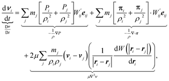 | (4) |
 . The first equation updates the SPH particle position. The second equation satisfies momentum balance in the fluid. Beneath each term is the corresponding term in the continuum equation of motion.
Since we are primarily interested in viscoelastic materials, then the local pressure tensor π(r,t) is not proportional to the instantaneous velocity gradient, but rather is some complicated functional of the velocity history. For example, π could be given by the upper-convected Maxwell model and the stress is given by the average of a function  (where Q is a conformation vector, nc is the polymer chain number density, and H is the entropic Hookean spring constant). In general, the probability density p(Ω; r,t) of some set of microstructural state variables Ω has an evolution equation involving the local velocity gradient. Hence, eqn (4) is supplemented by an evolution equation for the probability density at particle i
 | (5) |
![[script L]](https://www.rsc.org/images/entities/char_e144.gif) is an operator that depends on the particular molecular model. Note that there is only one approximation for ∇v that is thermodynamically consistent with eqn (3) and (4)
is an operator that depends on the particular molecular model. Note that there is only one approximation for ∇v that is thermodynamically consistent with eqn (3) and (4) | (6) |
For any such molecular model, one has  . In practice, one approximates eqn (5) to arbitrary accuracy with an ensemble of Nens independent trajectories of {Ωαi}, α = 1,..., Nαens. Then, our level of description is the set
  . In other words, each SPH particle i has a mass mi, a position ri, a velocity νi, and an ensemble of microstructural variables {Ωαi}.
The system of eqn (3) and (4) is closed by specifying a suitable equation of state for the pressure. We consider nearly incompressible flow and use30
Pi :![[thin space (1/6-em)]](https://www.rsc.org/images/entities/char_2009.gif) = c2ρi, = c2ρi, | (7) |
Even though the system of eqn ((3), (4) and (7)) is closed, we add one more—we also evaluate density as an additional variable instead of using the exact summation
 | (8) |
This approach was suggested by Monaghan39 in order to avoid problems concerning boundary and edge effects and also to save some computational cost by allowing all the variables to be evaluated in one step without an additional loop for the density calculation.
We implement a simple predictor–corrector method with explicit time-step where independent variables are evaluated at the predictor step and then the source is evaluated at the corrected step to get final values.40
3 Results and discussions
3.1 Method of manufactured solutions (MMS)
The accuracy of an SPH method, like many other Lagrangian methods, is hard to determine, but the method of manufactured solutions (MMS) verifies the algorithm, and shows that it is nearly second-order accurate in 2D space.In order to check the accuracy of SPH we use MMS for the classical problem of flow through a linear array of cylinders confined in a horizontal channel, Fig. 2. Periodic and no-slip boundary conditions are implemented at the sides, and top and bottom of the domains, respectively. The details of the calculations can be found in the Appendix.
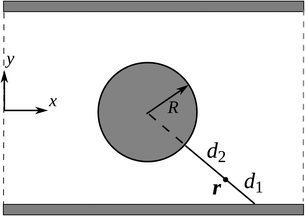 | ||
| Fig. 2 One period of an infinite array of cylinders confined in a horizontal channel. The radius R is used as the characteristic length. | ||
Fig. 3 shows side by side contour plots of the horizontal component of velocity vx of the manufactured solution in comparison with result of the SPH simulation, where 192 × 128 (besides the boundary particles) SPH particles are used. The top of Fig. 3 shows the analytic function that should be generated by the code using the derived source terms. The bottom of the figure validates our code.
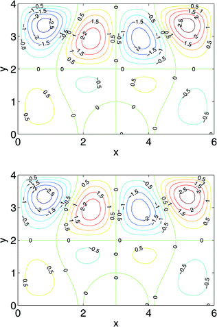 | ||
| Fig. 3 Comparison between the manufactured solution (top) and the numerical solution by SPH (bottom). | ||
3.2 Comparison against Newtonian asymptotic solution
After verifying the code with the MMS we check the performance of SPH by comparison of the simulation results with asymptotic solutions. We simulate Newtonian flow of a journal bearing, as depicted by the schematic in Fig. 4, for which an asymptotic solution is available42 was found by42 and is reproduced in the Appendix.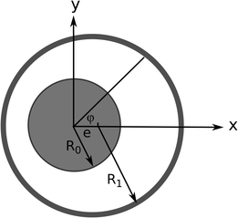 | ||
| Fig. 4 A journal bearing consists of two eccentric cylinders, and a fluid is trapped between as a lubricant. | ||
A journal bearing consists of two eccentric cylinders with a lubricating fluid in between. An assumption of infinitely long cylinders makes the problem two-dimensional. We define two dimensionless quantities—the eccentricity and the clearance ratio—as the ratio of the distance between the centers to the difference in the two radii, ε = e/(R1 − R0), and the ratio between the two radii minus 1, δ = R1/R0 − 1, respectively.
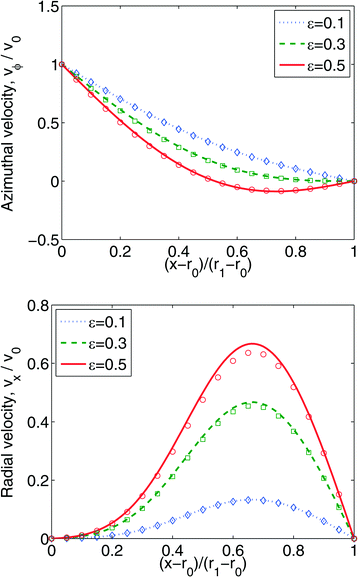
For δ = 0.1, we performed a series of simulations with ε = 0.1, 0.3, 0.5. The comparison of the steady state velocity profiles between obtained results and asymptotic solutions is shown in Fig. 5.
One can see that the agreement is good for the velocity in the azimuthal direction, but there are some deviations in the radial direction. We believe that this discrepancy is due to the clearance ratio's being insufficiently small (δ = 0.1) such that neglect of the higher-order terms is no longer warranted. On the other hand, it is not desirable to have smaller δ for SPH, since the particles in the narrowest strip will see two boundaries, which complicates implementation of boundary conditions. Nevertheless, we conclude that our SPH implementation is able to reproduce the results with acceptable accuracy.
3.3 Flow past a periodic array of confined cylinders
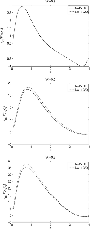
After checking that SPH can reproduce the manufactured solution, and a Newtonian asymptotic solution, a somewhat stronger test is to use SPH for a viscoelastic fluid. Here we use a benchmark problem: the flow past a periodic array of confined cylinders with the upper-convected Maxwell model (UCMM) for viscoelasticity.43 We take solvent viscosity ηs = 12.0 and polymer viscosity ηp = 8.0, resulting in a total dynamic viscosity of η0 = 20.0 and retardation ratio of ηs/η0 = 0.6. The initial constant reference density is taken to be ρ0 = 1.0. The flow is driven by a body force F = 1.0 × 10³ pointing in the positive x direction (see Fig. 2), resulting in a characteristic velocity v0 = 4.0 and Reynolds number approximately 0.2. A sound speed of 4.0 is used, and the density fluctuations are less than 1% at steady state. The dimensionless Weissenberg number is defined as Wi :![[thin space (1/6-em)]](https://www.rsc.org/images/entities/char_2009.gif) = λν0/R, which is a product of the polymer relaxation time and a characteristic strain rate. These parameters are comparable to those used in ref. 43. We perform simulations for Wi = 0.2, 0.6, 0.8, and use N = 2780, 11
= λν0/R, which is a product of the polymer relaxation time and a characteristic strain rate. These parameters are comparable to those used in ref. 43. We perform simulations for Wi = 0.2, 0.6, 0.8, and use N = 2780, 11![[thin space (1/6-em)]](https://www.rsc.org/images/entities/char_2009.gif) 020 SPH particles for different spatial resolutions. The Weissenberg number is changed by changing the relaxation time λ and fixing the body force and hence v0. Fig. 6 shows the dimensionless normal stress τxx along the symmetry line between two cylinders. Our comparison shows that it is harder for the stress to converge at higher values of Wi. These plots are comparable to Fig. 3 in ref. 43. Agreement with these prior results is taken as further validation of our implementation of SPH.
020 SPH particles for different spatial resolutions. The Weissenberg number is changed by changing the relaxation time λ and fixing the body force and hence v0. Fig. 6 shows the dimensionless normal stress τxx along the symmetry line between two cylinders. Our comparison shows that it is harder for the stress to converge at higher values of Wi. These plots are comparable to Fig. 3 in ref. 43. Agreement with these prior results is taken as further validation of our implementation of SPH.
3.4 Shear flow of entangled polymer melt
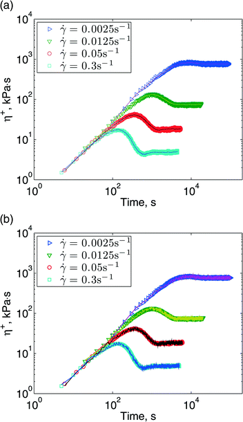
The upper-convected Maxwell model is the simplest viscoelastic model available to check our code. Now we replace it with a much more advanced model: the discrete slip-link model, for entangled polymers. Our first test is to simulate the uniform shear flow of a polymer melt using SPH, where each SPH particle contains 800 chains modeled with DSM. We compare the result with prior homogeneous flow calculations. A shear flow is created by moving a top plate at a constant speed while holding the bottom plate fixed. Once the flow reaches steady state, DSM is turned on. Because of statistical noise in DSM, the uniform shear flow may be altered by the polymer stress. We make two comparisons: in one, the polymer stress calculated by DSM is fed back to the flow, and in the other it is not. Results for different shear rates are shown in Fig. 7. One can see that predictions by DSM and SPH + DSM lie on top of each other for both cases. It is interesting that the calculations where flow and polymer stress are coupled show greater fluctuations.3.5 Journal bearing with polymer melt
After performing the above tests of our code, we can now predict something entirely novel as a first demonstration of application: the flow of a journal bearing with polymeric melt using the DSM model. Prediction of lubricant properties within a journal bearing is an important problem in engine manufacturing. It is well-known that use of non-Newtonian viscoelastic fluids as a lubricant can significantly influence (increase) the load-bearing capacity and the minimum oil film thickness.44,45 The problem has been extensively studied by different numerical techniques,46–49 but only with models unable to capture the rheology of realistic fluids quantitatively. Therefore, the problem is suitable for illustration of the proposed SPH + DSM method.For the fluid, we consider polystyrene of molecular weight MW = 238 kDa, and use the clustered slip-link model18 with β = 1 and the number of chain segments Nc = 30. We choose the characteristic time for a cluster of Kuhn steps to slide through an entanglement to be τc = 2.5 × 10⁻⁴ s, and the longest relaxation time of the entire chain is estimated to be τ = 0.01Nc3.48τc= 123 τc = 0.03075 s.50
We consider a journal bearing of eccentricity ε = 0.9 and clearance ratio δ = 0.06. The length and time scales are made dimensionless by the inner cylinder radius R0 and cluster characteristic time τc, respectively. The inner cylinder rotates at a constant angular velocity of Ω = 0.00325/τc = 13 s−1, resulting in a Weissenberg number  . We add N = 25
![[thin space (1/6-em)]](https://www.rsc.org/images/entities/char_2009.gif) 446 SPH particles to our domain, and each particle contains Nens = 800 chains. The polymer stress reaches steady state after approximately 10τ. We also performed calculations with Wi = 0.667 by reducing the shear rate to Ω = 0.000325/τc = 1.3 s−1.
446 SPH particles to our domain, and each particle contains Nens = 800 chains. The polymer stress reaches steady state after approximately 10τ. We also performed calculations with Wi = 0.667 by reducing the shear rate to Ω = 0.000325/τc = 1.3 s−1.
In ref. 46 stress on the inner cylinder and first normal stress coefficient were calculated numerically via the arbitrary Lagrangian–Eulerian (ALE) method, where the upper-convected Maxwell model (UCMM) and the Phan-Thien-Tanner (PTT) model were used to model the polymer contributions to stress. We consider the same set up and perform simulations with SPH + UCMM and SPH + DSM. The results are shown in Fig. 8, where on top we plot the shear stress on the journal, and on the bottom we plot the normal stress difference. The results reproduce the results of Gwynllyw et al.46 for UCMM. When DSM is used to model the polymer stress, the characteristic behavior of the stress has similar features—the location of peaks is similar for both models but the stresses are smaller in magnitude for DSM at both Weissenberg number values. Given the relative simplicity of the UCM model, the qualitative similarity is surprising.
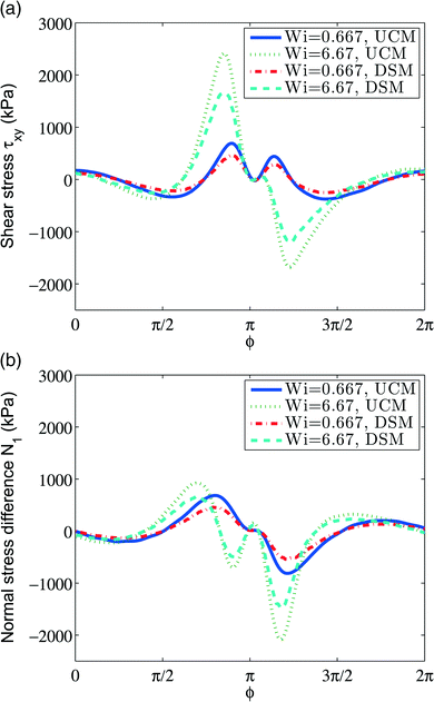 | ||
| Fig. 8 (a) Shear stress along the journal surface. (b) Normal stress difference along the journal surface. | ||
4 Conclusions
We simulated complex flows for entangled polymers based on the combination of a well-established macroscopic simulation technique, and successful molecular model—smoothed particle hydrodynamics and the discrete slip-link model. We first performed several tests of the proposed method: the method of manufactured solution was used to determine the accuracy of the SPH algorithm; we compared the results of a Newtonian simulation with an asymptotic analytical expression in a journal bearing; and the upper-convected Maxwell model in flow past an array of cylinders. All comparisons showed good agreement, validating our SPH algorithm. We also simulated uniform shear flow with SPH + DSM, and compared the results with prior homogeneous DSM calculations, which validates the combined code.As a proof of concept of the SPH + DSM approach we predict journal bearing flow with DSM parameters appropriate for a polystyrene melt. We also used the upper-convected Maxwell model UCMM instead of DSM in order to compare our predictions with the results of Gwynllyw et al.46 The performed tests show that the combination of the SPH method with the most detailed polymer model allows for accurate predictions in feasible computational time for non-trivial geometries. Since our approach is robust, other geometries are straightforward. For example, 3D flows with free surfaces are computationally feasible. Since DSM is also robust to chain architectures, flows of blends of branched and polydisperse linear chains, for example, could also be simulated.
The major limitation to our approach for simulating realistic processing conditions is the time needed to perform the simulation. In Table 1 we report simulation time for each test performed. The calculations were conducted on 32 CPUs, bound to 32 GPU cards (when DSM is used) in a one-to-one fashion. The most expensive simulation—journal-bearing flow of a polymer melt—used about 20 million chains and required 9 hours to finish. Shear flow simulations of 0.576 million chains of the same length (Nc = 30) took minutes to finish. For this Nc the technical limitation on one video card with 3 Gb memory can be estimated to be about 2.6 million chains. With an 84-GPU cluster available to us, the total number of simulated chains could be up to 220 million. Therefore, we used only about 10% of our resources. Clearly, time-dependent, three-dimensional flows under realistic processing conditions are accessible. Future work will examine more relevant applications to designing polymer materials where flow plays an important role.
| N | N ens | N × Nens | Wall time | |
|---|---|---|---|---|
| UCM flow past a cylinder | 11![[thin space (1/6-em)]](https://www.rsc.org/images/entities/char_2009.gif) 020 020 |
— | 11![[thin space (1/6-em)]](https://www.rsc.org/images/entities/char_2009.gif) 020 020 |
<1 h |
| DSM shear flow | 720 | 800 | 576![[thin space (1/6-em)]](https://www.rsc.org/images/entities/char_2009.gif) 000 000 |
<1 h |
| UCM journal bearing | 106![[thin space (1/6-em)]](https://www.rsc.org/images/entities/char_2009.gif) 783 783 |
— | 106![[thin space (1/6-em)]](https://www.rsc.org/images/entities/char_2009.gif) 783 783 |
261 min |
| DSM journal bearing | 25![[thin space (1/6-em)]](https://www.rsc.org/images/entities/char_2009.gif) 446 446 |
800 | ∼2 e7 | ∼9 h |
Several improvements on our implementation of SPH are possible. For example, explicit time-stepping could be substituted with an implicit time-step to gain some speed up in calculation time and increased stability. The evaluation of density, eqn (8), should be omitted to ensure conservation of mass; however, such an implementation also necessitates careful treatment of SPH particles near the boundaries to avoid edge effects. A larger ensemble size could be used to improve statistics.
A Details of SPH implementation
A.0.1 Kernel
Choosing a Gaussian support function is particularly useful for SPH, since derivatives and integrals are simple and can be written in terms of products involving the function itself. On the other hand, the Gaussian approaches zero asymptotically, and can be more expensive than polynomials. A good compromise is to use the analytic expressions for Gaussian support, and then approximate it everywhere by a polynomial. We use the quintic spline, which approximates a Gaussian form well.51We choose the smoothing length h to be 1.5 times the constant initial spacing between adjacent SPH particles. With this h, each SPH particle interacts with approximately 60 others in two dimensions. The operation count of the SPH algorithm, a generic N-body problem when using the non-compact Gaussian as the smoothing function, is reduced from O(N2) to O(N) by using the compactly supported quintic spline.
A.0.2 Time step
For time stepping, there are three criteria commonly used for step-size constraint in SPH. The first constraint is associated with the speed of sound—a Courant criterion to prohibit propagation of signal faster than the speed of sound.52 | (9) |
The second criteria comes from numerical integration and is due to particle acceleration,
 | (10) |
 | (11) |
B Details of method of manufactured solutions
In the method of manufactured solutions41 an analytic expression for the dependent variables (the “manufactured solution”) is fed into the equation of concern. Since the analytic expression is not the correct solution, it generates new source terms, which then are added to the algorithm. With the additional source terms the analytic “solution” should be generated numerically. In other words, a manufactured solution is an exact solution to some PDE or set of PDEs that has been constructed by solving the problem backwards. We are solving a differential equation of the form Dv = f, where D is the differential operator, v is the solution, and f is a source term. For the desired problem, f = 0. However, in MMS, one first manufactures a “solution” vm and then applies D to find the non-zero source term f :![[thin space (1/6-em)]](https://www.rsc.org/images/entities/char_2009.gif) = Dvm. The strength of this approach is that one can manufacture a general solution that performs a strong check on all the terms and coefficients of the equation.
= Dvm. The strength of this approach is that one can manufacture a general solution that performs a strong check on all the terms and coefficients of the equation.
We use a classical problem of flow through a linear array of cylinders confined in a horizontal channel as schematically shown in Fig. 2. The length is made dimensionless by the cylinder radius R. The channel has width 6 and height 4. To use MMS, we solve the system of equations
 | (12) |
 | (13) |
νx = −0.4![[thin space (1/6-em)]](https://www.rsc.org/images/entities/char_2009.gif) sin sin![[thin space (1/6-em)]](https://www.rsc.org/images/entities/char_2009.gif) (πx/3)sin(πy) + 1.2 (πx/3)sin(πy) + 1.2![[thin space (1/6-em)]](https://www.rsc.org/images/entities/char_2009.gif) sin(2πx/3)sin(πy/2), sin(2πx/3)sin(πy/2), | (14) |
νy = 2![[thin space (1/6-em)]](https://www.rsc.org/images/entities/char_2009.gif) sin(2πx/3)sin(πy/2) − 1.1 sin(2πx/3)sin(πy/2) − 1.1![[thin space (1/6-em)]](https://www.rsc.org/images/entities/char_2009.gif) sin(πx)sin(3πy/4). sin(πx)sin(3πy/4). | (15) |
This velocity v = (vx, vy) satisfies no-slip boundary condition on the two flat walls. To satisfy the similar boundary condition on the cylinder, we define v*(r) = d1ν(r)/(d1 + d2), where r, d1, d2 are depicted in Fig. 2. It is clear that vm :![[thin space (1/6-em)]](https://www.rsc.org/images/entities/char_2009.gif) = v − v* satisfies no-slip boundary condition on both the walls and the cylinder. We set the initial density to be unity, ρ0 = 1.0. This results in a Reynolds number on the order of O(1). We close the system of eqn (12) with the equation of state p = 1000ρ, resulting in a sound speed of 32.0. If we take the characteristic velocity to be the maximum of vm, this yields a Mach number of approximately 0.1 (recall that the density fluctuation scales like Mach number squared). The velocity vm are fed to eqn (12) to obtain the source terms for the density and momentum, then, SPH is used to solve the modified equation to check the accuracy. The simulation stops when the relative change in velocity between time steps,
= v − v* satisfies no-slip boundary condition on both the walls and the cylinder. We set the initial density to be unity, ρ0 = 1.0. This results in a Reynolds number on the order of O(1). We close the system of eqn (12) with the equation of state p = 1000ρ, resulting in a sound speed of 32.0. If we take the characteristic velocity to be the maximum of vm, this yields a Mach number of approximately 0.1 (recall that the density fluctuation scales like Mach number squared). The velocity vm are fed to eqn (12) to obtain the source terms for the density and momentum, then, SPH is used to solve the modified equation to check the accuracy. The simulation stops when the relative change in velocity between time steps,
 | (16) |
 | (17) |
C Details of analytic Newtonian flow in the journal bearing
The asymptotic solution is derived in the limit of vanishing clearance ratio and inertia, and the stream function is given by42 | (18) |
References
- J. Liu, X. Wang, D. Li, N. E. Coates, R. A. Segalman and D. G. Cahill, Macromolecules, 2015, 48, 585–591 CrossRef CAS.
- M. Culebras, C. M. Gómez and A. Cantarero, Materials, 2014, 7, 6701 CrossRef.
- D. N. Simavilla, J. D. Schieber and D. C. Venerus, J. Polym. Sci., Part B: Polym. Phys., 2012, 50, 1638–1644 CrossRef CAS.
- J. D. Schieber, D. C. Venerus and S. Gupta, Soft Matter, 2012, 8, 11781–11785 RSC.
- D. C. Venerus, J. D. Schieber, V. Balasubramanian, K. Bush and S. Smoukov, Phys. Rev. Lett., 2004, 93, 098301 CrossRef PubMed.
- J. D. Schieber, D. C. Venerus, K. Bush, V. Balasubramanian and S. Smoukov, Proc. Natl. Acad. Sci. U. S. A., 2004, 101, 13142–13146 CrossRef CAS PubMed.
- R. Noriega, A. Salleo and A. J. Spakowitz, Proc. Natl. Acad. Sci. U. S. A., 2013, 110, 16315–16320 CrossRef CAS PubMed.
- R. B. Bird, R. C. Armstrong and O. Hassager, Dynamics of Polymeric Liquids Vol I: Fluid Mechanics, Addison-Wesley, New York, 2nd edn, 1987 Search PubMed.
- J. D. Schieber, D. M. Nair and T. Kitkrailard, J. Rheol., 2007, 51, 1111–1141 CrossRef CAS.
- M. Andreev, R. N. Khaliullin, R. J. A. Steenbakkers and J. D. Schieber, J. Rheol., 2013, 57, 535–557 CrossRef CAS.
- R. Steenbakkers, C. Tzoumanekas, Y. Li, W. K. Liu, M. Kroger and J. Schieber, New J. Phys., 2014, 16, 010527 CrossRef.
- J. D. Schieber and M. Andreev, Annu. Rev. Chem. Biomol. Eng., 2014, 5, 367–381 CrossRef CAS PubMed.
- M. Kröger, Comput. Phys. Commun., 2005, 168, 209–232 CrossRef.
- S. Shanbhag and M. Kröger, Macromolecules, 2007, 40, 2897–2903 CrossRef CAS.
- I. Frederick, E. Bernardin and G. C. Rutledge, Macromolecules, 2007, 40, 4691–4702 CrossRef.
- F. L. Colhoun, R. C. Armstrong and G. C. Rutledge, Macromolecules, 2002, 35, 6032–6042 CrossRef CAS.
- M. Katzarova, L. Yang, M. Andreev, A. Cordoba and J. D. Schieber, Rheol. Acta, 2015, 54, 169–183 CrossRef CAS.
- M. Andreev and J. D. Schieber, Macromolecules, 2015, 48, 1606–1613 CrossRef CAS.
- S. F. Edwards, Proc. Phys. Soc., 1967, 92, 9–16 CrossRef CAS.
- M. Doi and S. F. Edwards, The Theory of Polymer Dynamics, Oxford University Press, 1988 Search PubMed.
- C. C. Hua and J. D. Schieber, J. Chem. Phys., 1998, 109, 10018–10027 CrossRef CAS.
- J. D. Schieber, J. Neergaard and S. Gupta, J. Rheol., 2003, 47, 213 CrossRef CAS.
- M. Andreev, R. N. Khaliullin, R. J. A. Steenbakkers and J. D. Schieber, J. Rheol., 2013, 57, 535–557 CrossRef CAS.
- M. Andreev, H. Feng, L. Yang and J. D. Schieber, J. Rheol., 2014, 58, 723 CrossRef CAS.
- R. N. Khaliullin and J. D. Schieber, Macromolecules, 2010, 43, 6202–6212 CrossRef CAS.
- E. Pilyugina, M. Andreev and J. D. Schieber, Macromolecules, 2012, 45, 5728–5743 CrossRef CAS.
- H. C. Öttinger, Beyond Equilibrium Thermodynamics, Wiley-Interscience, Hoboken, NJ, 2005 Search PubMed.
- A. Vázquez-Quesada, M. Ellero and P. Espanol, Phys. Rev. E: Stat., Nonlinear, Soft Matter Phys., 2009, 79, 056707 CrossRef PubMed.
- R. A. Gingold and J. J. Monaghan, Mon. Not. R. Astron. Soc., 1977, 181, 375–389 CrossRef.
- J. Morris, P. Fox and Y. Zhu, J. Comput. Phys., 1997, 136, 214–226 CrossRef.
- M. Ellero and R. Tanner, J. Non-Newtonian Fluid Mech., 2005, 132, 61–72 CrossRef CAS.
- L. Libersky, A. Petschek, T. Carney, J. Hipp and F. Allahdadi, J. Comput. Phys., 1993, 109, 67–75 CrossRef CAS.
- M. Grmela and H. C. Ottinger, Phys. Rev. E: Stat. Phys., Plasmas, Fluids, Relat. Interdiscip. Top., 1997, 56, 6620–6632 CrossRef CAS.
- A. Vazquez-Quesada, M. Ellero and P. Espanol, Microfluid. Nanofluid., 2012, 13, 249–260 CrossRef CAS.
- D. Auhl, J. Ramirez, A. E. Likhtman, P. Chambon and C. Fernyhough, J. Rheol., 2008, 52, 801–835 CrossRef CAS.
- J. D. Schieber and M. Andreev, Annu. Rev. Chem. Biomol. Eng, 2014, 5, 236–381 Search PubMed.
- J. Monaghan, Rep. Prog. Phys., 2005, 68, 1703–1759 CrossRef.
- J. Monaghan, J. Comput. Phys., 1994, 110, 399–406 CrossRef.
- J. J. Monaghan, Annu. Rev. Astron. Astrophys., 1992, 30, 543–574 CrossRef.
- M. Ellero, M. Kroger and S. Hess, J. Non-Newtonian Fluid Mech., 2002, 105, 35–51 CrossRef CAS.
- P. Roache, J. Fluids Eng., 2001, 124, 4–10 CrossRef.
- R. DiPrima and J. Stuart, J. Tribol., 1972, 94, 266–274 Search PubMed.
- A. Vazquez-Quesada and M. Ellero, J. Non-Newtonian Fluid Mech., 2012, 167–168, 1–8 CrossRef CAS.
- B. Williamson, K. Walters, T. Bates, R. Coy and A. Milton, J. Non-Newtonian Fluid Mech., 1997, 73, 115–126 CrossRef CAS.
- A. Berker, M. Bouldin, S. Kleis and W. van Arsdale, J. Non-Newtonian Fluid Mech., 1995, 56, 333–345 CrossRef CAS.
- D. Gwynllyw and T. Phillips, J. Non-Newtonian Fluid Mech., 2008, 150, 196–210 CrossRef CAS.
- G. W. Roberts and K. Walters, Rheol. Acta, 1992, 31, 55–62 CrossRef.
- X. Huang, N. Phan-Thien and R. Tanner, J. Non-Newtonian Fluid Mech., 1996, 64, 71–92 CrossRef CAS.
- D. Grecov and J.-R. Clermont, J. Non-Newtonian Fluid Mech., 2005, 126, 175–185 CrossRef CAS.
- M. Katzarova, L. Yang, M. Andreev, A. Córdoba and J. Schieber, Rheol. Acta, 2015, 54, 169–183 CrossRef CAS.
- J. J. Monaghan and J. C. Lattanzio, Astron. Astrophys., 1986, 158, 207 Search PubMed.
- W. Press, S. Teukolsky, W. Vetterling and B. Flannery, Numerical Recipes in C: The Art of Scientific Computing, Cambridge University Press, 1992 Search PubMed.
| This journal is © The Royal Society of Chemistry 2016 |

