Fusion of genomic, proteomic and phenotypic data: the case of potyviruses

Abstract

Data fusion has been widely applied to analyse different sources of information, combining all of them in a single multivariate model. This methodology is mandatory when different omic data sets must be integrated to fully understand an organism using a systems biology approach. Here, a data fusion procedure is presented to combine genomic, proteomic and phenotypic data sets gathered for Tobacco etch virus (TEV). The genomic data correspond to random mutations inserted in most viral genes. The proteomic data represent both the effect of these mutations on the encoded proteins and the perturbation induced by the mutated proteins to their neighbours in the protein–protein interaction network (PPIN). Finally, the phenotypic trait evaluated for each mutant virus is replicative fitness. To analyse these three sources of information a Partial Least Squares (PLS) regression model is fitted in order to extract the latent variables from data that explain (and relate) the significant variables to the fitness of TEV. The final output of this methodology is a set of functional modules of the PPIN relating topology and mutations with fitness. Throughout the re-analysis of these diverse TEV data, we generated valuable information on the mechanism of action of certain mutations and how they translate into organismal fitness. Results show that the effect of some mutations goes beyond the protein they directly affect and spreads on the PPIN to neighbour proteins, thus defining functional modules.

---

1. Introduction

Complex networks are widely used nowadays to model systems in several fields, e.g. sociology, physics, technology, or linguistics.^1,2 However, it is in biology, with the omics revolution, where complex networks are being applied in a broader range (metabolomics, proteomics, genomics…). The case of protein–protein interaction networks (PPINs) is of special interest. PPINs represent a map of physical contacts or functional interactions between proteins.³ Graphs are the most commonly used tool to visually represent these maps, the nodes being the proteins of the network, and the edges their interactions. For this, graph theory^1,2 is usually applied to extract statistical and topological descriptors from the PPINs as a first step. Then, other graph theory tools, usually applied on social or computer complex networks (e.g. clustering algorithms⁴), are used to identify functional modules within the network.

The present work is carried out using the case of potyviruses. Potyvirus is the largest genus within the Potyviridae family, containing more than 180 different members. Indeed, the Potyviridae are among the most common plant RNA viruses.⁵ Potyviruses have a single-stranded, positive-sense RNA genome of approximately 10 kilobases (kb). Their genomes encode for eleven different proteins: P1, HC-Pro, P3, 6K1, CI, 6K2, VPg, NIaPro, NIb, CP, and P3N-PIPO. Its PPIN is composed of the interactions established at different stages of the infectious cycle between these eleven proteins. Since biological activity usually arises from the association of several proteins, it is crucial to relate these elements (proteins and interactions) to a biological function or a phenotype. In this study, the data are obtained from a collection of 20 Tobacco etch virus (TEV) single nucleotide substitution mutants and 53 double mutants resulting from the pairwise combination of the single ones.⁶ For each of these 73 mutant genotypes, absolute fitness was evaluated in its natural host Nicotiana tabacum var Xanthi nc during a single infection cycle.⁶ Complementarily, a PPIN inferred from empirical protein–protein interaction (PPI) data from several potyviruses⁷ is used to relate the mutations and the organismal fitness. A mutation in a protein may change (slightly or dramatically) its ability to perform its biological functions correctly. The mutated TEV proteins establish interactions with other viral proteins according to the PPIN of potyviruses.⁷ Since viral proteins are multifunctional, and they carry out some of their functions as protein complexes, it is reasonable to assume that a part of the effect of the mutated protein on the fitness is channelled through its PPIs. In other words, mutations affect PPIs, which ultimately affect biological fitness. Some mutations are much more harmful while others have no fitness effect. The PPIN of Potyvirus adds biological context to the mutation and allows for a deeper analysis of the importance of each protein in the virus' infectious cycle.

Some assumptions are made in the present approach. The main one is that each mutation affects all the PPIs of a mutated protein in the same way. Probably the true modifications are subtler, depending also on other factors. Proteins are highly heterogeneous structures and modifications in different parts of their sequence may have different biological consequences for different interactions. However, the lack of available data and their nature constrained the present study. The problem revolves around two issues. On the one hand, there are protein residues or domains that are much more sensitive to mutations than others. Mutations in some locations, such as the catalytic site of an enzyme, are potentially much more harmful to its function than mutations affecting other domains. In this study we have data available for only 73 mutants for a genome of 10 kb encoding for eleven proteins. Instead of relating mutants and fitness directly, the present approach relates mutants to fitness using proteins and interactions between them as a way to channel those effects and hopefully obtain useful information. Even with a relatively small pool of mutants it is possible to apply the proposed methodology and obtain valid results.

On the other hand, very scarce information is available for particular interactions. One way to include variability in the influence of a particular mutation on each interaction could be carrying out a docking study. Having structural information of two proteins it would be possible to estimate the influence that any change in their sequences has on a possible docking between them. Unfortunately, none of the TEV proteins have been crystallographically determined so this analysis is not possible yet. Therefore, until no new proteomic information arises, the influence of mutations is spread equally to all the interactions that the mutated protein establishes.

The problem of relating different sources of data has been widely assessed in systems biology using data fusion. Data fusion can be defined as a statistical procedure to analyse simultaneously different sources of complex data sets.⁸ This methodology has been applied to identify genes related to specific diseases,⁹ to PPINs and gene expression,¹⁰ to fuse gene regulatory networks, transcriptional factors and amino acid sequences,¹¹ for metabolic profiling¹² and for biomarker search in proteomics.¹³ One of the most used methods in data fusion^12–16 is Partial Least Squares regression¹⁷ (PLS), which pursues to relate a set of biological descriptors or process variables and a set of biological outputs or quality variables taking advantage of the existing correlations among them.

The aim of the present work is to fuse genomic, proteomic and phenotypic data of potyviruses in a single multivariate model to understand the relationships among the different data sources. This way, the objective is to relate mutated proteins, their effect on the PPIN, and the resulting organismal fitness measured under controlled laboratory conditions. Fig. 1 shows a scheme of the data fusion. In this case, the mutations and the PPIN are the explanatory variable data blocks, and the fitness measured for each mutant take the role of the dependent variable. Finally, a set of functional modules of the PPIN is isolated using the PLS modelling. The purpose of this approach is to gain insight into the molecular interactions that occur during the virus infection more than to construct a robust predictive model. Similar grey models have been proposed during the last few years, using exploratory^18,19 and predictive methods,²⁰ dealing with metabolic networks. To improve the predictive power of the model we would need more genetic and proteomic information, such as the analysis of codon usage and, specially, the characterization of the protein structure. Unfortunately, this information is not available at the moment.

Fig. 1 Schematic representation of the study. The aim of this paper is to relate the mutations generated on the genome of TEV, their effect on the protein–protein interaction network, and the resulting phenotypic fitness of the virus in vivo.

The rest of the paper is organised as follows. The Results section presents the results of the data fusion approach of the reconstructed and mutated PPIN of Potyvirus, the mathematical and statistical modelling, and the relevant modules of the network. Some conclusions on the analysis and future lines are drawn in Discussion and conclusions section. Finally, further information on the methodology and the reconstructed PPIN of Potyvirus can be found in Methods section.

2. Results

The following subsections explain in detail the data acquisition and the mathematical and statistical modelling. First, the PPIN of Potyvirus is built, based on an exhaustive literature review.⁷ Then, the effects of mutations on the fitness of TEV are measured in the natural host N. tabacum. Finally, the effect of the mutations on the PPIN is mathematically modelled, and the three sources of data (mutations, PPINs and fitness) are related using a multivariate statistical projection method.

2.1. Protein–protein interaction network reconstruction

All currently available PPIs of Potyvirus were gathered as an initial step.⁷ These data were obtained from six different articles published over the last few years.^21–26 In the original dataset 681 PPIs were tested, 194 PPIs were detected among the 11 viral proteins. Integrating these data from different sources in a common pool required some statistical standardization and pre-processing. To determine which interactions were relevant and an accurate representation of the Potyvirus' PPIN topology a relevance coefficient was defined (more details in ref. 7). From this analysis, a complete and biologically significant PPIN of Potyvirus was built. This network (Fig. 2) is used here to relate mutations and organismal fitness and to extract information about the biological importance of proteins and their interactions.

Fig. 2 PPINs of Potyvirus. Eleven proteins (represented as circles) and their 25 detected interactions (represented as double-arrows).

2.2. Mutations and fitness

The collection of single and double mutants used in this work was reported in ref. 6. Twenty single nucleotide substitution mutants and 53 double mutant genotypes of TEV form the dataset analysed here. The fitness of these mutants had been previously quantified by means of growth assays in the natural host N. tabacum. Fitness is a measure that captures the ability of a mutant virus to grow and spread through the plant during an infection cycle relative to the ability of the unmutated wild type virus.²⁷

The collection of mutants was generated at random and thus it is somehow irregular, not affecting all TEV proteins: 6K1, CP and P3N-PIPO were not mutated (see Table 1). Moreover, some proteins like P1 and VPg were mutated more times than others such as 6K2, CI and NIb. Although a more complete collection of mutants would be very useful to further increase the accuracy of our findings, the collection of 73 mutants used for this study is a fair representation of the TEV genome and its 11 proteins.

Table 1 Mutations experimentally generated on the genome of TEV

Mutation	Protein	Type	# of mutants
PC2	P1	Nonsynonymous	2
PC6	P1	Nonsynonymous	7
PC7	P1	Nonsynonymous	5
PC12	P1	Nonsynonymous	4
PC19	HC-Pro	Synonymous	10
PC22	HC-Pro	Nonsynonymous	6
PC26	HC-Pro	Synonymous	4
PC40	P3	Synonymous	5
PC41	P3	Nonsynonymous	4
PC44	P3	Synonymous	5
PC49	CI	Nonsynonymous	8
PC60	CI	Synonymous	3
PC63	6K2	Nonsynonymous	10
PC67	VPg	Nonsynonymous	4
PC69	VPg	Nonsynonymous	13
PC70	VPg	Nonsynonymous	5
PC72	VPg	Nonsynonymous	3
PC76	NIaPro	Synonymous	8
PC83	NIb	Nonsynonymous	10
PC95	NIb	Nonsynonymous	10

---

The mutant collection has some features that make it an interesting and appropriate starting point for the data fusion. Six of the 20 single mutants correspond to synonymous mutations. In other words, the nucleotide substitution does not translate in an amino acid replacement in the protein sequence. In spite of being synonymous, some of these mutations had a significant effect on fitness²⁷ due to RNA stability, enhanced RNA silencing responses or improved translational efficiency, among other possibilities. Although these mutations have no effect on the protein sequence and thus no predictable effect on the PPIN either, they represent a natural source of fitness variability that is taken into account in our results. Other particularity of the data is that lethal mutations exist, meaning those that render zero fitness for the virus bearing them, i.e. these mutations do not allow the virus to survive and grow. Nine of the double mutations are lethal. These mutations are excluded from the analysis because, if included, they will mask all the variability of non-lethal mutations varying fitness in a discrete manner.

The effect of the mutations on the proteins can be quantified using different information. The most precise way to do it would be using structural information. Having the resolved structure of the viral proteins, it is possible to change a particular amino acid and observe how that change affects some structural variables. Some mutations would increase the stability of the protein and some would decrease it, defining a magnitude for the mutation. Unfortunately, as it was mentioned before, none of the TEV proteins has been crystallized making this approach unfeasible. Another approach consists of assuming that biochemically different amino acids would induce more severe perturbations in the structure conformation. This way a mutation changing an amino acid for another very similar would produce only a slight structural disturbance and consequently only a minor protein activity variation. An extremely different amino acid would produce a much more dramatic change in the protein activity.

To represent the biochemical similarity or the distance between the original amino acid in the sequence and the new one produced by the mutation we used an empirical amino acid substitution matrix. These matrices describe the rate at which one amino acid changes to any other over time. These matrices are commonly used in the field of protein sequence alignment, calculating the probability that a particular amino acid changes over time to a new one through mutation. The underlying idea is that an amino acid substitution is more likely to survive to the filter of selection if it is similar to the original amino acid than if it is physically very different. Similar amino acids would then preserve a similar folding structure and activity for the protein. Thus, we used the information contained in the entries of these matrices to quantify the magnitude of each mutation. Since the collection of mutants available is composed of single and double nucleotide mutations it seemed to be appropriate to use the Point Accepted Mutation²⁸ (PAM) matrix to compute the distances generated by the mutations. These matrices were developed using observed mutations in closely related proteins. Large numbers in the PAM matrix denote substitutions very likely to be removed by purifying natural selection, thus unlikely to persist in the long-term evolutionary time. Since the mutants used for this study have almost identical sequences it seemed to be more precise to use a low number PAM matrix. For this, we decided to use the PAM2 matrix²⁸ to quantify the effect of the amino acid replacement on viral proteins. It was assumed that mutations with high PAM2 values would induce a strong disruption in the protein structure and, therefore, would have a high probability to negatively affect its biological function.

2.3. Mathematical modelling

Once the distance produced by each mutation is computed from the PAM2 matrix, the effect of the mutation on the PPIN has to be modelled. However, as commented previously, some mutations result in a zero distance (synonymous mutations). Since these mutations have no effect on the network, they may directly affect fitness without crossing the PPIN. The distances generated by all mutations are provided in additional file 1 (ESI†), jointly with the fitness measured for all mutants.

The distance registered for all nonsynonymous mutations is modelled as follows. The distance generated by an amino acid replacement, which affects a particular protein, weakens the existing interactions between the influenced one and its first-step neighbours in the PPIN. Fig. 3 shows a small example of this modelling concept. If a mutation is produced on protein A, with a registered distance j, the interactions relating A to its neighbours, B and C, are weakened as follows:

where A∼B and A∼C mark the interaction between A and B, and A and C, respectively, and U is the reference value, which refers to the maximum value in the entire PAM2 matrix. In other words, the maximum distance an amino acid change defines.

Fig. 3 Small example of the mutation modelling. Initially, all detected interactions between proteins have a value 1. When a mutation is performed on protein A with distance j, the intensity of the PPIs A∼B and A∼C is lowered by j/U.

It is worth noting that the distance produced in the protein is a measure of how different is the protein after mutation. Then, this distance is translated into a strength/intensity measure in the network between the protein and its first-step neighbours. So no distance is being considered between different proteins in the PPIN.

The different data sources presented in this study must be combined properly to be analysed using a latent structure method. Since PLS, in its original form, works with two-way data matrices, the information collected on the previous subsections must be arranged in such a way that each individual (i.e. experiment) is represented by rows, and the different types of variables (i.e. mutations, interactions and fitness) by columns. So three data matrices are built: the mutation matrix M has the 20 different mutations as variables, the interaction matrix I has the intensity in each of the 25 interactions by columns, and the vector y has the fitness registered for each individual. All matrices have 64 rows, corresponding to the non-lethal mutants. Fig. 4 presents an example of the matrices defined above, following the small PPIN taken as an example in Fig. 3. In this case three individuals are considered, e.g. in Exp1 a nonsynonymous mutation is performed on protein A, producing a distance j and registering a fitness y₁. Note that on Exp3 a synonymous mutation on protein A is performed, therefore, it has no effect on I, i.e. neither A∼B nor A∼C are lowered in this case.

Fig. 4 Data matrices. Matrices M, I and vector y have the information from the mutations, interactions and fitness, respectively. Three examples are presented. On Exp1 a nonsynonymous mutation is performed on A, with distance j, and fitness y₁. A nonsynonymous mutation on D is performed in Exp2, producing a distance k and fitness y₂. On Exp3 a synonymous mutation is performed in A, producing no distance (and no effect on I), and a fitness y₃. The colours correspond to the data sources described in Fig. 1.

2.4. Statistical modelling

The data matrices built in the previous subsection can be analysed using different statistical techniques. Considering only mutations and fitness, a design of experiments (DOE) can be performed, but this approach presents some drawbacks here. There are 20 different mutations performed individually or two-by-two, across the original 73 individuals. A model including only mutations and fitness could be fitted using penalized regression (such as Lasso²⁹ or Elastic Net³⁰) to prevent rank deficiency problems. However, it is known that the PPIs affect the fitness, so in the previous approach this effect is not taken into account.

The other possible approach consists of relating all the interaction strengths/intensities to the fitness, using classical linear regression. The problem is that the mutations are performed on different proteins affecting different interactions, which may not be comparable in this model.

In this work, a PLS regression is applied to fuse the genomic, proteomic and phenotypic data in a single multivariate model, the first two sources being the explanatory variable blocks and the phenotypic fitness of the dependent variable. Using a PLS model, the available data are compressed into a set of latent variables that relates mutations and interactions to the observed fitness. This allows us to clarify which mutations, and also which sections of the network, increase or decrease the fitness of TEV.

The different data sources, detailed in previous subsections, have to be pre-processed in order to obtain meaningful components in the PLS model. In the present case the dataset is directly autoscaled, i.e. the variables are centred and divided by their standard deviation to have mean 0 and standard deviation 1.

Regarding the statistical modelling, the PLS model can be strongly (and harmfully) affected by some of the mutants compiled for the present study. As commented above, lethal mutations decrease the fitness straight to zero, while for the non-lethal mutations it oscillates in a small range around the fitness of the wild-type virus. The inclusion of the lethal ones in the study will force the model to explain only the variation between the lethal and non-lethal, pointing simply to the mutations that have been lethal. To avoid this spurious result, and explain equally the positive and negative effect of the mutations and interactions on the fitness of TEV, these lethal genotypes have been removed from the datasets. This relates directly to the way in which mutation severity is quantified. PAM matrices are constructed assuming non-lethal scenarios. Even the most extreme amino acid substitution is quantified as a prerequisite of biological success. Therefore it is sensible to exclude the lethal mutations from the main analysis, since the benchmark chosen to represent mutation magnitude excludes them originally.

Once the data are prepared for the analysis, a PLS model is fitted using the software ProSensus ProMV.³¹ To decide how many components extract from the data, the cross-validation criterion using seven groups is selected (more details in Methods section). The aim of this criterion is to choose the number of components that offers the highest predictive power.

First, a PLS model including all variables is fitted. Later on, a reduced PLS model is obtained by deleting some mutations and interactions that have a very low influence on the fitness. These mutations are PC12, PC67, PC69, and PC72. The PPIs deleted are: HC-Pro∼VPg, VPg∼VPg, VPg∼NIaPro and VPg∼CP. Basically, these variables have a non statistically significant PLS regression coefficient in the first PLS model (95% of confidence level). The results of the first PLS model can be found in additional files 2 and 3 (ESI†).

Table 2 shows the results of the reduced PLS model. For the analysis, matrices M and I are merged in a single matrix X, including all the variables collected in the study. With a 3-component model, 30.1% of the variability in X explains 78.3% of variance in the fitness, y, with a predictive ability of 56.7%. It is worth noting that although network topology is definitely a major contributor to the variance of the fitness, there are some other factors that are not included in this particular approach, harming the predictive power of the PLS model. RNA structure stability and codon usage bias are two clear examples of important contributors to fitness that are not included in the analysis.

Table 2 PLS regression results (reduced model). Cumulative variances in X = [M I] and y explained by the model (R²X and R²y, respectively) and predictive power of the model (Q²)

Component	R ^2 X cumulative (%)	R ^2 y cumulative (%)	Q ^2 cumulative (%)
1	11.8	57.6	39.5
2	23.4	70.0	46.7
3	30.1	78.3	56.7

---

Fig. 5 shows the PLS regression coefficients of the variables in the dataset. The red bars mark the statistically significant PPIs and mutations. The relevant ones are chosen based on the 95% Jackknife confidence intervals computed for their corresponding PLS regression coefficient.³² In this way, when the interval does not include zero, the variable has a relevant effect on the fitness, either positive or negative, with a 95% confidence level.

Fig. 5 PLS regression coefficients. For each regression coefficient, the 95% Jackknife confidence interval is shown. The statistically significant variables are plotted as red bars. The mutations with a relevant effect on the fitness are PC6, PC19, PC22, PC63 and PC83. The significant PPIs are: P1∼CI, P1∼VPg, HC-Pro∼HC-Pro, HC-Pro∼NIaPro, 6K2∼NIaPro, NIaPro∼NIb, NIb∼NIb, and NIb∼CP.

PC22 has a statistically significant negative effect on the resulting fitness of TEV; i.e. when this mutation is generated in the genome, the fitness lowers its value (see Fig. 5). PC6, PC19, PC63, and PC83 also affect fitness, but in a positive direction. The fitness increases when either of these mutations is present in TEV genome. It is worth noting that a PLS model using only the mutations and the fitness identifies basically the same relevant mutations as the combined mutations–interactions model, but with less explained variance and predictive power in fitness (70.1% and 47.0%, respectively).

The PPIs P1∼CI, P1∼VPg, 6K2∼NIaPro, NIaPro∼NIb, NIb∼NIb, and NIb∼CP have a statistically significant negative effect on the fitness (see Fig. 5). Bearing in mind the mathematical modelling, when a mutation is performed, the corresponding interactions lower their values. So, the lower is the value of the interaction, the higher is the fitness computed. Alternatively, HC-Pro∼HC-Pro and HC-Pro∼NIaPro have a statistically significant positive effect on the fitness, i.e. the lower is the value of the interaction, the lower is the fitness computed.

All the statistically significant variables, mutations and PPIs, are summarized in Table 3. This information will be valuable to define the functional modules in the next subsection.

Table 3 Statistically significant explanatory variables. ± superindices mark the positive/negative effect of the variable on the fitness

Mutation	Protein affected	Interactions
PC6^+	P1	P1∼C1^−, P1∼VPg^−
PC63^+	6K2	6K2∼NIaPro^−
PC83^+	NIb	NIb∼NIaPro^−, NIb∼NIb^−, NIb∼CP^−
PC22^−	HC-Pro	HC-Pro∼HC-Pro^+, HC-Pro∼NIaPro^+
PC19^+	HC-Pro	(Synonymous mutation)

---

2.5. Functional modules

On the previous subsection, the explanatory variables, PPIs and mutations with a statistically significant effect on the organismal fitness, are identified among the rest of the variables registered. In order to finally establish the relationships among the three data sources, following the scheme proposed in the Introduction section (see Fig. 1), the genomic-proteomic-phenotypic effect must be explained using the information in Table 3. If the relevant mutations and PPIs are represented on the original PPIN (see Fig. 6) some interesting conclusions can be drawn.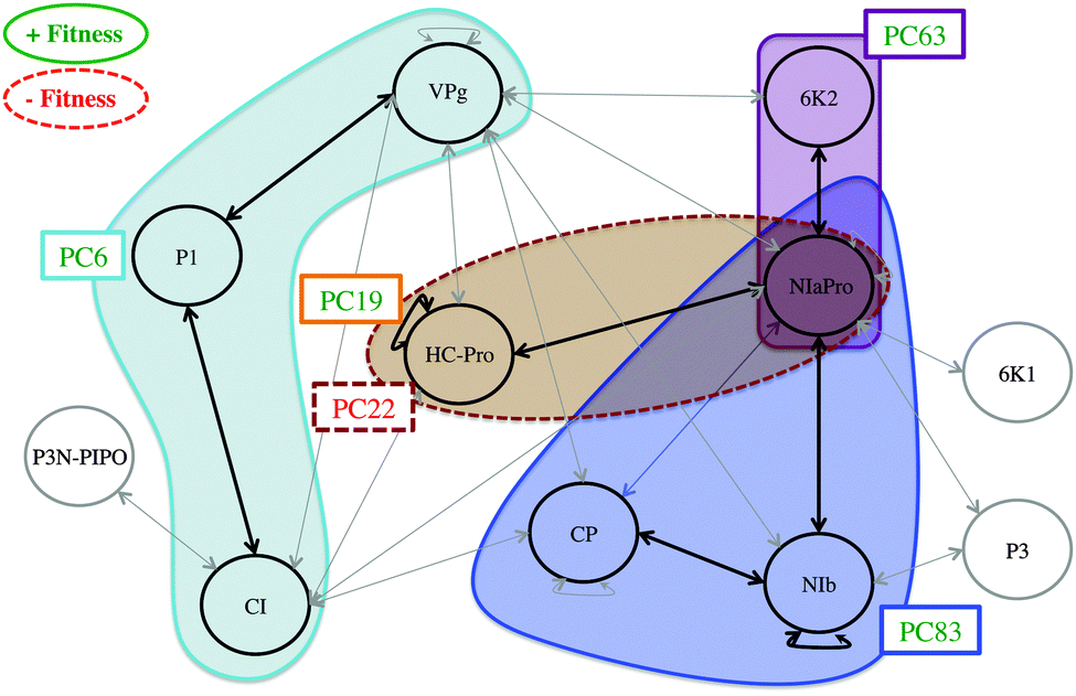

Fig. 6 Functional modules of TEV. The cyan module is activated via mutation PC6 in protein P1 and affects proteins CI and VPg. The violet module is activated by mutation PC63 on protein 6K2 and affects protein NIaPro. The blue module is activated via mutation PC83 in protein NIb and affects NIb, CP and NIaPro. The brown module is activated via mutation PC22 in protein HC-Pro and affects HC-Pro and NIaPro. The synonymous mutation PC19 is performed in HC-Pro. Mutation PC22 has a negative effect on the fitness while the rest of the mutations have a positive effect.

Mutation PC6, affecting protein P1, is positively correlated with TEV fitness. At the same time, interactions P1∼VPg and P1∼CI are also relevant in the PLS model, being negatively correlated with viral fitness. These mutation-fitness effects and interaction-fitness effects represent a unified mutation-interaction-fitness effect. Fig. 7 shows a scheme of this process: when PC6 is generated on P1, the interactions with its neighbours VPg and CI lower their values, and the fitness is increased as a result. A cyan ellipse in Fig. 6 rounds this functional module.

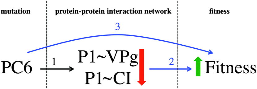Fig. 7 Diagram of mutation – PPIN – fitness effects. The mathematical modelling implies that, when mutation PC6 is applied, the protein–protein interactions P1∼VPg and P1∼CI lower their values (1). The data fusion results indicate that: (i) when PC6 is applied the fitness increases (2), and (ii) when the previous interactions lower their values, the fitness increases (3). The mathematical and statistical modelling are describing the effect of the mutation on the protein–protein interaction network and the effect of the network on the fitness.

This behaviour is also observed with the blue and violet modules (see Fig. 6). The former one is activated via mutation PC83 on protein NIb, and affects NIb, NIaPro and CP. The latter starts with mutation PC63 on 6K2, affecting only its relationship with NIaPro. When these sections are activated, the fitness increases. In this way, Fig. 7 can also represent the behaviour observed in these modules, replacing the mutation and interaction names.

Two mutations affecting HC-Pro have a statistically significant effect. When mutation PC22 is generated, the PPIs HC-Pro∼HC-Pro and HC-Pro∼NIaPro are affected (brown module in Fig. 6) and the phenotypic fitness decreases. Alternatively, PC19 is positively correlated with the fitness: when it is introduced in HC-Pro, the fitness increases significantly. Both mutations are compatible with the mathematical modelling because PC19 is a synonymous mutation, and therefore it has no effect on the PPIN network. Fig. 8 shows the different effects related to HC-Pro. This modelling would be infeasible if PC19 were a nonsynonymous mutation. In this hypothetical case, since it would affect HC-Pro∼HC-Pro and HC-Pro∼NIaPro, it would be incoherent that the mutation increases the fitness and its associated interactions lower its value at the same time.

Fig. 8 Diagram of mutations – PPIN – fitness effects in the case of multifunctional protein HC-Pro. The mathematical modelling implies that, when mutation PC22 generated in HC-Pro, the protein–protein interactions HC-Pro∼HC-Pro and HC-Pro∼NIaPro lower their values (1). The data fusion results indicate that: (i) when PC22 is introduced the fitness decreases (2), and (ii) when the previous interactions lower their values, the fitness decreases (3). When PC19 is generated, the fitness increases (6). All the effects described in this diagram are coherent among them because PC19 is a synonymous mutation; therefore it has no effect on the protein–protein interaction network (4 and 5).

Two comments are here in due regarding the functional modules (Fig. 6). Firstly, if an interaction between two proteins is included in a module (e.g. P1∼CI) it implies that the effect of the interaction on the fitness is statistically significant, considering that it can be activated by nonsynonymous mutations performed on both proteins (i.e. P1 and CI). However, the effect is stronger when the mutation defining the module is performed (i.e. PC6 on P1), since the mutation is activating other relevant interactions (i.e. P1∼VPg). Secondly, if an interaction activated by a key mutation is not included in the corresponding module (i.e. interaction 6K2∼VPg, activated via mutation PC63) it implies that the effect of the interaction, considering that it can be activated by nonsynonymous mutations performed on both proteins (i.e. 6K2 and VPg), is not statistically significant.

High-level and mid-level data fusion procedures obtain separate models and extract relevant features of each data matrix, respectively, to combine them in a fused model to predict the biological output.³³ In this study, however, we decide to apply a low-level data fusion, concatenating row-wise, matrices M and I because the mathematical modelling applied here establishes a direct relationship between the mutations and the PPIN, so the joint analysis of both matrices in a single PLS model leads us to identify functional modules exploiting not only the mathematical modelling but also the topological interactions being affected by the different mutations.

3. Discussion and conclusions

The PLS modelling applied to genomic, proteomic and phenotypic data sets allows us to integrate the mutations performed on viral proteins, their effects on the PPIN, and their influences on the organismal fitness experimentally quantified. In this way, three biological functional modules affecting the PPIN and influencing the fitness positively have been detected. Two additional modules are identified affecting a single protein. One influences the protein network, being negatively correlated with the organismal fitness. The other one has a positive effect on the fitness without affecting the PPIN. This implies that different mutations affecting the same protein induce different behaviours in the activity of the PPIN and the resulting fitness.

Classical clustering algorithms usually work with a standalone version of the network, detecting dense sections of the topology based solely on its interaction intensities (or basically on node degrees). In comparison to traditional clustering, the presented methodology allows working with different sources of information, combining them to squeeze the data and extract the relevant information. With this data fusion, (i) the mutations are related to topological changes in the network and their subsequent influence on the fitness, and (ii) the mutations not affecting the network can also be related to the fitness.

Data fusion reveals as a very powerful tool to analyse and relate different types of biological information. The larger the network and the collection of mutants, the more precise its findings are. The present study, analysing a relatively small PPIN (11 nodes and 25 interactions) and a small number of combinations of mutations (64 out of the 210 possible ones), results in a quite high-explained variability. However, there are intrinsic biological considerations that limit the scope of the method. These considerations, such as RNA stability, efficiency inducing the antiviral RNAi response of the plant and codon usage bias may be included in the model as additional sources of variability but much more data would be needed. Besides this, further work of interest includes testing the proposed methodology with a larger dataset containing more mutants, and extending the analysis to larger PPINs, in order to build multivariate models with a higher predictive power, exploiting the features of the projection to latent structure methods.

4. Methods

4.1. Amino acid substitution matrix

Describing and measuring the severity of the mutations produced in TEV genome is essential for applying the data fusion methodology in this work. As it was briefly commented before, the PAM2 amino acid substitution matrix is used to quantify the potential severity that a mutation produces in the virus. Although PAM2 is based on evolutionary changes over time, and it is used more often in sequence alignment methods, it is still a valuable and proved source of information regarding the likelihood of amino acid substitutions. It is assumed that if a determined change from a particular amino acid to another one is evolutionarily unlikely it is because such a change is potentially more disturbing to the protein function. Alternatively, evolutionarily common amino acid replacements are assumed to have a minor impact on the protein structure.

We used the scores in the matrix to quantify the effect of the mutations on each of the 73 mutants used in the present study (eqn (1)). Each mutation gives a value that represents the difference between the substitution of a particular amino acid by itself (meaning no mutation at all) and the new amino acid in the sequence. For instance, mutation PC2 produces an amino acid change between F and C. The matrix establishes a score of nine for the F to F substitution (no change) and −30 for the F to C substitution. The difference (39 in this example) between these values represents how similar (chemically and structurally) both amino acids are. We then normalized that value for all mutations with the maximum possible value for a change among the 20 amino acids (W to E replacement, with a difference value of 47). Since, in the absence of epistatic interactions, double mutants are potentially twice as harmful as single mutants, in order to compare all mutants (single and double) we chose as a normalizing value 2 × 47 = 94.

Eqn (1) then gives a value between 0 and 1 that expresses how potentially disturbing is the mutation for the protein (being 0 the most aggressive and 1 the least). This approach is a rough way to translate qualitative (mutations and amino acid changes) into quantitative data. The way these quantitative data are used later would imply that when a particular mutation is given the value of 0 the function of the protein is totally eliminated. However, this is unlikely to happen: even with very severe mutations the proteins may perform their functions with some lesser degree. This approach should be taken as an indication of the direction that the protein function may take. On the other hand, proteins are very complex and heterogeneous structures and therefore some areas of the sequence may be particularly sensible to changes (catalytic sites, docking areas, etc.). Unfortunately, the 3D structure information needed to precisely quantify this severity is not yet available for any TEV protein.

4.2. Partial least squares regression (PLS)

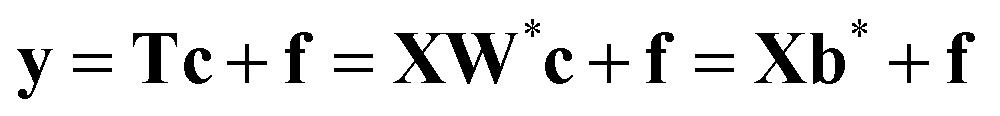
Partial least squares regression (PLS) is a multivariate projection method commonly applied to model the relationships between a set of X variables (descriptors or process variables) and a set of Y variables (output or quality variables) reducing significantly the dimensionality of the initial data set. The PLS model finds a set of latent variables (LVs) that both describe the X data and predict the Y data, with the aim of maximising their covariance.

In the present study, since the Y data comprise only a single variable y (fitness), the PLS-1 version of PLS regression is applied. When the number of Y-variables increases, these variables have to be projected in the same manner as the X ones (more details in ref. 17 and 34). The first step of PLS-1 consists of obtaining the scores of X as linear combinations of its original variables (eqn (2)).

T = XW* (2)

where W* is the weighting matrix of the X variables.

These new variables are, multiplied by the loadings matrix P, good summaries of X, i.e. the residual matrix E in the equation X = TP^T + E, have small entries. Additionally, the T variables are built in such a way¹⁷ that they are good predictors of y. Then, the y variable can be expressed as follows:

where c is the loading vector of y, f is the residual vector and b* is the PLS regression coefficient vector.

4.3. Cross-validation and Jackknife confidence intervals

Cross-validation (CV) is a resampling technique widely used in statistics and chemometrics.³⁵ The aim of CV is to assess the number of relevant components to be extracted in the multivariate model. This procedure groups the observations, in the present study into seven groups, and then fits as many PLS models as groups, leaving each time a single group out. Then, the sum of squares of the differences between the actual fitness values and the predicted ones is used to estimate the predictive ability of the model.¹⁷ CV is usually performed one component after another, until the predictive power of the model decreases.

Simultaneously with the CV, the Jackknife confidence intervals for the PLS regression coefficients are computed, at a confidence level of 95%, from all models fitted.³² These intervals are built based on the estimated PLS regression coefficients of each round of the CV.

4.4. Software

The PLS model and the correspondent plots shown in the present study are built using ProSensus ProMV³¹ version 14.0.8.

Author's contributions

GB and AF-F performed the analyses and wrote the manuscript. JP and AF conceived the study and reviewed the manuscript. SFE conceived the study and wrote the manuscript. All authors read and approved the final manuscript.

Acknowledgements

This work was supported by the Spanish Ministerio de Economía y Competitividad grants BFU2012-30805 (to SFE), and DPI2011-28112-C04-02, DPI2011-28112-C04-01, DPI2014-55276-C5-1-R (to AF and JP) and by Generalitat Valenciana grant PROMETEOII/2014/021 (to SFE). The first two authors are recipients of fellowships from the Spanish Ministerio de Economía y Competitividad: BES-2012-053772 (to GB) and BES-2012-057812 (to AF-F).

References

1. R. Albert and A.-L. Barabási, Rev. Mod. Phys., 2002, 74, 47–97.
2. M. E. J. Newman, SIAM Rev., 2003, 45, 167–256.
3. J. De Las Rivas and C. Fontanillo, PLoS Comput. Biol., 2010, 6, e1000807.
4. Z. Wang and J. Zhang, PLoS Comput. Biol., 2007, 3, e107.
5. A. Gibbs and K. Ohshima, Annu. Rev. Phytopathol., 2010, 48, 205–223.
6. J. Lalić and S. F. Elena, Heredity, 2012, 109, 71–77.
7. G. Bosque, A. Folch-Fortuny, J. Picó, A. Ferrer and S. F. Elena, BMC Syst. Biol., 2014, 8, 129.
8. I. Van Mechelen and A. K. Smilde, Chemom. Intell. Lab. Syst., 2010, 104, 83–94.
9. S. Aerts, D. Lambrechts, S. Maity, P. Van Loo, B. Coessens, F. De Smet, L.-C. Tranchevent, B. De Moor, P. Marynen, B. Hassan, P. Carmeliet and Y. Moreau, Nat. Biotechnol., 2006, 24, 537–544.
10. Y. Nie and J. Yu, BMC Syst. Biol., 2013, 7, 49.
11. J. Baumbach, S. Rahmann and A. Tauch, BMC Syst. Biol., 2009, 3, 8.
12. Y. Xu, E. Correa and R. Goodacre, Anal. Bioanal. Chem., 2013, 405, 5063–5074.
13. J. Forshed, M. Pernemalm, C. S. Tan, M. Lindberg, L. Kanter, Y. Pawitan, R. Lewensohn, L. Stenke and J. Lehtiö, J. Proteome Res., 2008, 7, 2332–2341.
14. H. W. Lee, A. Christie, J. Xu and S. Yoon, Biotechnol. Bioeng., 2012, 109, 2819–2828.
15. J. Rojas, A. F. Tachon, D. Chevalier, T. Noguer, J. L. Marty and C. Ghommidh, Sens. Actuators, B, 2004, 102, 284–290.
16. A. Conesa, J. M. Prats-Montalbán, S. Tarazona, M. J. Nueda and A. Ferrer, Chemom. Intell. Lab. Syst., 2010, 104, 101–111.
17. S. Wold, M. Sjöström and L. Eriksson, Chemom. Intell. Lab. Syst., 2001, 58, 109–130.
18. J. M. González-Martínez, A. Folch-Fortuny, F. Llaneras, M. Tortajada, J. Picó and A. Ferrer, Chemom. Intell. Lab. Syst., 2014, 134, 89–99.
19. A. Folch-Fortuny, M. Tortajada, J. M. Prats-Montalbán, F. Llaneras, J. Picó and A. Ferrer, Chemom. Intell. Lab. Syst., 2015, 142, 293–303.
20. A. R. Ferreira, J. M. L. Dias, A. P. Teixeira, N. Carinhas, R. M. C. Portela, I. A. Isidro, M. von Stosch and R. Oliveira, BMC Syst. Biol., 2011, 5, 181.
21. E. Zilian and E. Maiss, J. Gen. Virol., 2011, 92(12), 2711–2723.
22. L. Lin, Y. Shi, Z. Luo, Y. Lu, H. Zheng, F. Yan, J. Chen, J. Chen, M. J. Adams and Y. Wu, Virus Res., 2009, 142, 36–40.
23. D. Guo, M.-L. Rajamäki, M. Saarma and J. P. T. Valkonen, J. Gen. Virol., 2010, 82, 935–939.
24. W. T. Shen, M. Q. Wang, P. Yan, L. Gao and P. Zhou, Acta Virol., 2010, 54, 49–54.
25. S.-H. Kang, W.-S. Lim and K.-H. Kim, Mol. Cells, 2004, 18, 122–126.
26. M. L. M. Yambao, C. Masuta, K. Nakahara and I. Uyeda, J. Gen. Virol., 2003, 84(10), 2861–2869.
27. P. Carrasco, F. de la Iglesia and S. F. Elena, J. Virol., 2007, 81, 12979–12984.
28. M. O. Dayhoff and R. M. Schwartz, Atlas of Protein Sequence and Structure, 1978, 5, 345–358.
29. M. A. Rasmussen and R. Bro, Chemom. Intell. Lab. Syst., 2012, 119, 21–31.
30. H. Zou and T. Hastie, J.R. Statist. Soc. B, 2005, 67(2), 301–320.
31. ProMV 12.0.1 Software Retrieved from ProSensus, http://www.prosensus.ca/solutions/multivariate-analysis-software, 2012.
32. B. Efron, Biometrika, 1981, 68, 589–599.
33. L. M. C. Buydens, The Analytical Scientist, 2013, 813, 24–30.
34. P. Geladi and B. R. Kowalski, Anal. Chim. Acta, 1986, 185(C), 1–17.
35. S. Wold, Technometrics, 1978, 20, 397–405.

---

Footnote

† Electronic supplementary information (ESI) available: Molecular BioSystems. Additional file 1. Mutations performed on TEV, distances registered and fitness measured. Additional file 2. PLS regression results (first model). Additional file 3. PLS regression coefficients (first model). See DOI: 10.1039/c5mb00507h

---