Kinetic and thermodynamic study of polyaniline functionalized magnetic mesoporous silica for magnetic field guided dye adsorption

Abstract

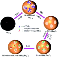
An eco-friendly magnetic mesoporous silica iron oxide (MS@Fe₃O₄) nanoparticles with a high surface area was fabricated using a colloidal chemical method. Hereafter, polyaniline (PANI) was conjugated into the pores of MS@Fe₃O₄ to obtain PANI–MS@Fe₃O₄ nanocomposites. The nanocomposites were essentially monodispersed and highly efficient for the adsorption of methyl orange (MO). In addition, the rate of the adsorption reaction followed pseudo-second-order kinetics and the adsorption isotherm fitted well to the Langmuir isotherm model. The negative values for the change in Gibbs energy (ΔG) and positive value of the change in enthalpy (ΔH) indicated that the overall adsorption process was spontaneous and endothermic in nature. The density functional theory calculation using the Gaussian 09 and GaussView 5.0 programs also supported the electrostatic interaction phenomena between PANI and MO, which is mainly responsible for the adsorption.

---

1. Introduction

Over the last two decades, mesoporous silica (MS) has served as the material of choice in many applications because of its unique characteristics such as high surface area,¹ large pore volumes and uniform pore sizes.² Recently, metal oxide@MS core shell nanocomposites have been extensively used and have been widely studied.^3–5 One class of these nanocomposites, mesoporous silica coated iron oxide (MS@Fe₃O₄) nanoparticles, have been recognized as a significant material in many fields including catalysis,⁶ biomedical engineering⁷ and environmental remediation.⁸ Discrete nanocomposites with a magnetic core and porous shell structures are given specific attention because of their high surface areas, large amount of accessible pore volume and easy separation by an external magnetic field. However, the applications of pure silica materials are limited because of the presence of a lesser number of functional groups on the mesopore surface. The surface properties of pure MS materials are therefore required to be amended by incorporating species with the desired functionalities. The functions of the organic group determine the properties of the MS materials such as surface reactivity, adsorption capacity and enhanced stability. A variety of functional groups, such as amino,⁹ carboxylic acid,¹⁰ thiol¹¹ and sulfonic acid,¹² have been introduced into silica matrices for diverse applications. In this investigation, the magnetic MS have been functionalized by amine and imine groups through polyaniline (PANI) modification.

Among the conducting polymers, PANI is the most intensively studied candidate for industrial applications because of its easy synthesis, good environmental stability,¹⁴ low cost¹³ and high conductivity.¹⁵ To date, a number of PANI conjugates have been successfully used for diverse applications.^16,17 For example, Li et al. prepared graphene/PANI nanocomposites, where PANI was sandwiched between layers of graphene sheets and the nanocomposites were investigated as supercapacitors.¹⁶ Bogdanovic et al. employed an in situ polymerization technique to synthesize cheaper copper–PANI nanocomposite materials and then investigated its antimicrobial properties.¹⁷ But there are few reports on the PANI modified magnetic MS nanocomposites. Therefore, it was necessary to investigate the nanocomposites and their importance. In this research, functionalized PANI on the surface of magnetic MS was prepared by a simple oxidative polymerization technique and subsequently the nanocomposite was used for an adsorption study.

Industrial effluents discharging into the hydrosphere are harmful when brought into contact with living tissues for a long time. Dyes, the most harmful industrial effluents, reduce the penetration of sunlight into the water bodies and consequently prevent photosynthesis in the aqueous flora and fauna.¹⁸ Dyes are also endangering public health by direct use of water polluted by them, as well as by eating aquatic organisms that live in the polluted water resource. Different physico-chemical methods have been proposed for the removal of dyes from aqueous solutions. Out of the possible techniques, the adsorption process is established as the most attractive and efficient method for the removal of organic dyes from waste water because of its low cost,¹⁹ simple operational conditions and better performance.²⁰ Various adsorbents, such as activated carbon, alumina, metal hydroxide, zeolite, and MS, have been used to remove azo dyes from wastewater.^21–23 However, there is still a need to search for a low cost adsorbent to develop a green, simple and rapid synthesis for organic dye adsorption. In this context, porous magnetic nanoparticles with high surface area conjugated with PANI for the adsorption of anionic dyes has been developed. In this study, methyl orange (MO) is used as a model effluent compound because it is widely used in the textile, papermaking and leather industries and is harmful to society.²⁴

2. Materials and methods

2.1 Materials

Iron(III) chloride (anhydrous), iron(II) sulfate heptahydrate, ammonium hydroxide, tetraethyl orthosilicate (TEOS) and ammonium persulfate (APS), MO, aniline, hydrochloric acid (HCl), ethanol, methanol, benzene, N,N-dimethylformamide (DMF), n-hexane and N-cetyl-N,N,N-trimethylammonium bromide (CTAB) were procured from Merck. Millipore grade water was used throughout the experiments. The stock solution of MO was prepared in water and diluted to the required concentrations.

2.2 Methods

The synthesis of PANI–MS@Fe₃O₄ was performed according to our previously reported procedure,²⁵ which was composed of three steps. Firstly, Fe₃O₄ magnetic nanoparticles were synthesized using a co-precipitation method. Secondly, the core shell (MS@Fe₃O₄) structure was constructed by silica coating and the generation of pores on the surface of the silica coated magnetic nanoparticles. Finally, polymerization of aniline was performed onto MS@Fe₃O₄ to achieve the PANI–MS@Fe₃O₄ nanocomposite.

2.2.1 Synthesis of MS@Fe₃O₄. Fe₃O₄ and MS@Fe₃O₄ nanoparticles were synthesized according to our previously published procedure.²⁵ For a sheer silica coating on Fe₃O₄, the resulting Fe₃O₄ nanoparticles were homogeneously dispersed in a mixture of 80 mL of ethanol, 20 mL of water and 1 mL of concentrated ammonia solution (28%) for 30 minutes. Subsequently, 0.03 g of TEOS was dropped to the stirred mixture. After 6 h the product was separated and repeatedly washed with a water/ethanol mixture. For further generation of pores on the surface of the silica coated Fe₃O₄ nanoparticles, the product was redispersed in a mixture of 80 mL water, 70 mL of absolute ethanol, 0.3 g CTAB and 1.2 mL of ammonia solution (28%). After 30 minutes 0.4 g TEOS was added dropwise and stirring was continued for a further 6 h at room temperature. The product was collected using a magnetic concentrator and washed repeatedly with a water/ethanol mixture. CTAB was removed by stirring the product obtained in 105 mL of an ethanolic mixture containing 5 mL of 2 M HCl for 12 h. The MS@Fe₃O₄ core shell nanoparticles were collected using a magnetic concentrator and repeatedly washed with ethanol followed by drying at 60 °C.

2.2.2 Synthesis of PANI–MS@Fe₃O₄. MS@Fe₃O₄ nanoparticles (0.1 g) were added to a mixture of 0.1 g aniline and 1 mL of hexanol. After 24 h, 0.2 g of APS dissolved in 2 mL of 1 N HCl were added dropwise into the solution with stirring at a low temperature of 0–5 °C. After 2 h of stirring, the suspension was moved to a low temperature for 12 h. Finally the product was collected using a magnetic concentrator and washed with ethanol followed by drying at 60 °C.

2.3 Characterization

The surface functional groups of the silica coated Fe₃O₄, MS@Fe₃O₄, PANI–MS@Fe₃O₄ and MO adsorbed PANI–MS@Fe₃O₄ were investigated using Fourier-transform infrared (FTIR) spectroscopy (Thermo Nicolet Nexus 870 FTIR spectrometer). A Raman spectrum was recorded with a Nicolet Almega XR dispersive raman spectrometer using a Nd:YAG laser source with a wavelength of 532 nm. The phase formation and crystallographic state of these particles were determined using Phillips PW 1710 X-ray diffractometer (XRD) with nickel-filtered Co-Kα radiation (λ = 1.79 Å). The morphological characterization was performed using scanning electron microscopy (SEM; Jeol JSM-6340F) and transmission electron microscopy (TEM; Phillips CM 200). The nitrogen (N₂) adsorption and desorption isotherms were obtained at 77 K using a Quantachrome NOVA 3200e instrument. Prior to adsorption, the samples were degassed properly. Energy-dispersive X-ray spectroscopy (EDS) was carried out using an Oxford Instruments X-Max. The absorption spectra of MO was measured using a Shimadzu UV-1800 ultraviolet-visible spectrophotometer with an operating voltage of 220–240 V/50–60 Hz.

2.4 Dye adsorption study

The experiments used to study adsorption were performed in the water phase to investigate the effect of different parameters such as time (1–6 min), initial pH (2–9), temperature (303–323 K), initial dye concentration (4–32 mg L⁻¹) and adsorbent dose (0.001–0.005 g). In general, 0.003 g of PANI–MS@Fe₃O₄ nanocomposites was added to 10 mL of MO solution (20 mg L⁻¹) and a shaker (Tarsons Spinix Orbital Shaker) with constant shaking of 180 rpm was used according to the method protocol. The effect of temperature on the adsorption behavior of PANI–MS@Fe₃O₄ was investigated using a Rivotek Incubator Shaker at 110 rpm. After equilibrium, the clear supernatant solution was collected using magnetic lixiviation and the decrease in absorbance of the supernatant solution was measured using a UV spectrophotometer at 463 nm. The percentage dye removal efficiency (R_e) was calculated using the following equation:^26,27

The adsorption capacity of PANI–MS@Fe₃O₄ at equilibrium, q_e (mg g⁻¹), was calculated using the equation:²⁸

where C₀ and C_e are the initial and equilibrium liquid phase concentrations (mg L⁻¹) respectively; V is the volume of dye solution taken (L); W is the weight of adsorbent taken (g).

2.5 Dye desorption study

The experiments made to study desorption were conducted by dispersing the dye adsorbed PANI–MS@Fe₃O₄ in a methanol solution containing 4% acetic acid.²⁶ The percentage dye desorption (D_e) was calculated using the equation:

2.6 Density functional theory and adsorption energy calculation

Gaussian 09 (ref. 29) and GaussView 5.0 (ref. 30) software packages were used to perform electronic structure calculations and visualization. The ground state electronic structure of PANI and MO was optimized using density functional theory (DFT) in its unrestricted forms, employing the STO-3g* level set. Electron correlations were included in the DFT calculation using Becke-3–Lee–Yang–Parr (B3LYP) procedure^31–33 which includes Becke's gradient exchange corrections, and the Lee, Yang and Parr correlation function.³⁴ No symmetry constraint was imposed during the geometry optimization. Absence of imaginary frequencies confirmed that the optimized geometries are stable.

PANI, MO and the PANI*MO complex were optimized at the unrestricted BLYP (UBLYP)/STO-3g* level of theory. PANI was optimized by putting a positive charge on the alternating nitrogen atoms. MO was also optimized by specifying the negative charge on one oxygen atom in the SO₃⁻ group.

To understand the electrophilic and nucleophilic attack of PANI by MO, the molecular electrostatic potential map (MEP) of PANI and MO was calculated by using UBLYP/STO-3g* level of theory as shown in the Fig. 1. The red color represents the negative diffusion region whereas the blue color represents the positive diffusion region. All the nitrogen in PANI possesses a positive diffusion region while in the MO, the negative charge is concentrated on the SO₃⁻ group. It is clear from Fig. 1 that a strong attraction exists between the N–H groups of PANI and the SO₃⁻ head of the MO molecule. The optimized structure of the PANI*MO complex, calculated at the same level of theory is shown in the Fig. 2(a). From the MEP of PANI*MO complex (shown in Fig. 2(b)) it is clear that there is an extensive electronic overlap between the PANI and MO primarily via 80O–24H–23N. Weak interactions were also visible through other oxygen atoms of the SO₃⁻ group and the C–H proton of the aromatic ring. A high negative complexation energy (−11.05 kcal mol⁻¹) confirmed the presence of a strong interaction between PANI and MO. During the process of optimization, a proton detached from one of the nitrogen atoms (23N) of PANI which subsequently attached to the (80O) SO₃⁻ group of the MO. A clear picture of a 24H shift from 23N to 80O can be visualized by plotting the 23N–24H and 80O–24H bond distance against the optimization steps. Variation of the 23N–24H and 80O–24H bond distance with the optimization steps are shown in the electronic ESI Fig. S1.† Initially the 23N–24H bond distance was 1.020 Å, which by increasing the optimization steps, can be increased and optimized at 1.5097 Å. This signifies the movement of 24H away from the 23N atom. While initially the 80O–24H distance was 2.6767 Å by increasing the optimization steps, the distance started to reduce and was optimized at 1.0838 Å signifying the shifting of 24H towards the 80O and formation of the 80O–24H bond.

Fig. 1 Chemical structure of PANI and MO with the corresponding molecular electrostatic potential (MEP) map of PANI and MO with an iso value 0.004.

Fig. 2 Fully optimized geometry of the PANI*MO complex obtained at the DFT/UBLYP/STO-3g* level of theory (a). Corresponding MEP at iso value 0.04 (b).

The interaction energy between the PANI and MO were evaluated by using the following equation:

ΔE_interaction(PANI*MO) = E(PANI*MO) − E(PANI) − E(MO) (4)

where ΔE_interaction(PANI*MO) = the formation energy change of the PANI*MO complex, E (PANI) = the energy of PANI and E(MO) = the energy of MO and E(PANI*MO) = the energy of the PANI*MO complex.

The formation of a new O–H bond and the presence of a number of electrostatic interactions makes a high change in energy during the complex formation between PANI and MO. The change in energy during the complexation from individual components is 164.4074 kcal mol⁻¹. But after the formation of the new complex where MO is protonated and PANI is deprotonated, the complexation energies becomes −25.60 kcal mol⁻¹ (raw) and −11.05 kcal mol⁻¹ (corrected), respectively, and the basis set superposition error corrected interaction energies were 0.023185660755 Hartree.

3. Results and discussion

3.1 Characterization of the magnetic adsorbent

The transmission FTIR spectra of silica coated Fe₃O₄, MS@Fe₃O₄, PANI–MS@Fe₃O₄, MO adsorbed PANI–MS@Fe₃O₄ and MO for the range 4000–400 cm⁻¹ are shown in Fig. 3. In the finger print region, the characteristic band of Fe–O vibration at 585 cm⁻¹ (ref. 35) can be associated with the sustainability of the magnetic core even after pore formation on silica and MO adsorption. This indicates that magnetic nanoparticles were not affected during the washing of CTAB using an ethanol HCl mixture. In addition the spectral peak at around 3400 cm⁻¹ corresponds to surface-sorbed water or hydroxyl groups.^36,37 In the spectra of silica related materials, asymmetric and symmetric vibrations of Si–O stretching were observed at 1088 cm⁻¹ and 810 cm⁻¹, respectively.^38,39 The characteristic peaks of PANI at 810, 1305, 1494, and 3250 cm⁻¹ were attributable to C–H, C–N˙⁺, C=C, and N–H bonds, respectively for the quinoid and benzenoid rings present in PANI.^25,40 The characteristic peaks at 1235, 1305, and 1581 cm⁻¹ indicated that PANI is conjugated in its emeraldine form.⁴¹ The bare MO shows that absorption bands at 628 cm⁻¹ and 810 cm⁻¹ are the characteristics of S=O stretching vibration, and the C–H aromatic out-of-plane bending, respectively.⁴² In addition, the N=N stretching band⁴² for MO emerges at 1625 cm⁻¹. The emergence of all these bands of MO (Fig. 3(e)) qualitatively confirms the adsorption of MO into PANI–MS@Fe₃O₄ nanocomposites.

Fig. 3 Transmission FTIR spectra of silica coated Fe₃O₄ (a), MS@Fe₃O₄ (b), PANI–MS@Fe₃O₄ (c), MO adsorbed PANI–MS@Fe₃O₄ (d) and MO only (e).

The Raman pattern of PANI–MS@Fe₃O₄ is displayed in Fig. 4(a). The spectrum shows three peaks at 410, 440, 512, and 574 cm⁻¹, which were attributed to the magnetic core.^43,44 The broad band at 806 cm⁻¹ refers to benzene ring deformation. In addition, the strong band appearing at 1587 cm⁻¹ is related to C=C stretching vibration in the quinonoid ring. The peak of highest intensity at 1488 cm⁻¹ is ascribed to the C=N stretching vibration of the quinonoid ring. The bands at 1334 cm⁻¹ and 1166 cm⁻¹ correspond to the C–N⁺˙vibration of the delocalized polaronic structures and C–H bending vibration of the semi-quinonoid ring.

Fig. 4 Raman spectra of PANI–MS@Fe₃O₄ (a), XRD patterns of Fe₃O₄ (b), PANI–MS@Fe₃O₄ (c), and MS@Fe₃O₄ (d).

Fig. 4(b–d) show the wide angle XRD patterns of Fe₃O₄, PANI–MS@Fe₃O₄ and MS@Fe₃O₄ respectively, in which the diffraction peaks corresponding to (220), (311), (400), (422), (511), and (440) at 30.1°, 35.8°, 43.1°, 53.6°, 57.09°, and 62.9° can be perfectly indexed to the phase of Fe₃O₄ (Joint Committee on Power Diffraction Pattern (JCPDP) 75-1609). The matching of the diffraction peaks of MS@Fe₃O₄ and PANI–MS@Fe₃O₄ with Fe₃O₄ suggested that the Fe₃O₄ nanoparticles were well retained in the silica matrix. The broad band at 20–25° in Fig. 4(c) and (d) can be assigned to the amorphous silica shell. Two less intense peaks at 20.2° and 25.08° in Fig. 4(c) are because of the slight crystalline nature of the as synthesized emeralidine salt form of PANI.^45,46 Thus, the FTIR and XRD data support the theory that the as synthesized PANI in PANI–MS@Fe₃O₄ is in the emeralidine salt form.

The SEM image of the PANI–MS@Fe₃O₄ nanocomposite is shown in Fig. 5(a). The as synthesized nanocomposites were regularly spherical with a mean diameter of 160–170 nm and a rough surface. Additionally, in the TEM image of MS@Fe₃O₄ the inorganic–organic core shell structure can be clearly visualized because of the different electron penetrability between the magnetic nanoparticle and the silica shell. The black portion refers to the magnetic core whereas the grey portion with an average thickness of 20–25 nm refers to the silica layer.

Fig. 5 SEM image of PANI–MS@Fe₃O₄ (a) and TEM image of MS@Fe₃O₄ (b).

Fig. 6 shows the N₂ adsorption–desorption isotherms of MS@Fe₃O₄, PANI–MS@Fe₃O₄, and MO adsorbed PANI–MS@Fe₃O₄. According to the IUPAC classification the isotherms obtained are of typical type IV isotherms.^47,48 As expected, the Brunauer–Emmett–Teller (BET) surface areas were calculated to be 779.27 m² g⁻¹ for MS@Fe₃O₄, 425.65 m² g⁻¹ for PANI–MS@Fe₃O₄ (ref. 25) and 195.072 m² g⁻¹ for MO adsorbed PANI–MS@Fe₃O₄. A possible explanation for the decrease of surface area values is related to the conjugation of PANI into the pores of MS@Fe₃O₄ and further adsorption of MO into the PANI–MS@Fe₃O₄.

Fig. 6 N₂ adsorption–desorption isotherms of MS@Fe₃O₄ (a), PANI–MS@Fe₃O₄ (b) and dye adsorbed PANI–MS@Fe₃O₄ nanocomposites (c).

Purity of the Fe₃O₄ core, presence of the silica shell, conjugation of PANI and adsorption of MO was confirmed using the EDS technique and the corresponding results for Fe₃O₄, MS@Fe₃O₄, PANI–MS@Fe₃O₄ and MO adsorbed PANI–MS@Fe₃O₄ are shown in Fig. 7. The peaks of Fe and O appeared in all spectra corresponding to Fe₃O₄, while the peaks of Si in Fig. 7(b–d) could be attributed to the silica coating. The N peak observed in Fig. 7(c) is the signature of the successful conjugation of PANI into MS@Fe₃O₄. Compared to PANI–MS@Fe₃O₄, MO adsorbed PANI–MS@Fe₃O₄ showed additional peaks of S and Na, which confirm the adsorption of MO. The C signals in Fig. 7(a–c) could be expected to be from the carbon tap used during the sample preparation.

Fig. 7 EDS spectra of Fe₃O₄ (a), MS@Fe₃O₄ (b), PANI–MS@Fe₃O₄ (c) and dye adsorbed PANI–MS@Fe₃O₄ (d).

3.2 Effect of pH on adsorption of MO

Many researchers have reported the significant role of pH in adsorption efficacy^49,50 because it exerts a profound influence on the adsorption tendency of the adsorbate molecule presumably because of its influence on the surface charge and functional groups of the adsorbent as well as the ionization/dissociation of the adsorbate molecules.⁵¹ For that reason, batch experiments were conducted at different pH ranges from 2.0 to 9.0 at room temperature and the effect of pH on the percentage removal of MO, is shown in Fig. 8(a) and (b). A variable pH was obtained by adding the requisite amount of 0.1 M HCl or 0.1 M sodium hydroxide. Results indicate that the adsorption of MO into PANI–MS@Fe₃O₄ is fairly pH dependent and the maximum adsorption efficiency (96.96%) was achieved at pH 4. The pK_a value of MO is reported to be 3.4 and at a pH < pK_a, the MO predominantly exists in an anionic form and subsequently it gets protonated. On the other hand, because of the basic nature of nitrogen containing functionalities (imine group –N=, pK_a = 2.5 and amine group –N=, pK_a = 5.5),⁵² PANI gets positively charged in an acidic medium. It is, therefore, at pH 2 and pH 3 that the electrostatic repulsion occurred between the positively charged nanocomposites and protonated MO, which results in a decline in adsorption (63.1% at pH 3 and 42.5% at pH 2). However, MO, at pH > pKa, exists in an anionic form and maximum adsorption (96.96%) was achieved at pH 4. This is because of the intensive electrostatic attraction established between the positive part of PANI and the anionic MO. Above pH 4, adsorption declines gradually up to pH 7 and then decreased slightly to become almost constant above pH 8. The competitive adsorption of hydroxyl on imine and amine groups might result in electrostatic repulsion with anionic MO, leading to low adsorption of MO at a basic pH.

Fig. 8 Effect of pH (a); inset is the effect of pH in the range pH 4 to pH 9 (b); temperature (c); initial MO concentration on the adsorption of MO on PANI–MS@Fe₃O₄ (d) and mass of adsorbent (e). {Temperature: 273 K for (a), (b), (d) and (e), initial MO concentration: 20 mg L⁻¹ (10 mL) for (a), (b), (c) and (e). PANI–MS@Fe₃O₄: 0.003 g for (a), (b), (c) and (e)}.

3.3 Effect of MO dose on adsorption

Fig. 8(c) shows the effect of the increase of concentration of dye on the percentage adsorption of PANI–MS@Fe₃O₄ nanocomposites. Results indicate that dye adsorption declined from 99.12% to 90.35% with an increase in dye concentration from 4 mg L⁻¹ to 32 mg L⁻¹ of dye. This is because of the decrease in the availability of effective adsorption sites on the adsorbent.⁴⁵

3.4 Effect of adsorbent dose on adsorption

The effect of adsorbent dosage on the adsorption of MO was evaluated using quantities of PANI–MS@Fe₃O₄ adsorbent ranging from 0.001 g to 0.005 g. Experimental data, as shown in Fig. 8(e), reveal that the MO adsorption was found to be lowest (77.45%) at an adsorbent dose of 0.001 g and sharply increases to 97.42% at an adsorbent dose of 0.003 g. Above this adsorbent dose, the adsorption becomes almost constant. Initially the increase in percentage adsorption with increase of adsorbent was attributed to the higher available surface area, consequently augmenting the number of active sites⁵⁴ available for MO adsorption.⁵⁵ Furthermore, the almost constant percentage of MO adsorption obtained from the adsorbent dose of 0.003 g is because of the aggregation of the active sites of the adsorbent. Therefore, the adsorbent dose was fixed at 0.003 g.

3.5 Effect of temperature on adsorption of dye

Temperature is another important parameter that affects the adsorption process by changing the diffusion rate of the adsorbate molecules, owing to decrease in the viscosity of the solution. Furthermore, it alters the equilibrium adsorption capacity (q_e) of the adsorbent.⁵⁶ So this series of experiments was carried out at five different temperatures, namely, 303 K, 308 K, 313 K, 318 K and 323 K. The observed values are shown in Fig. 8(c). As the temperature increases, the removal efficiency of the dye increases and consequently q_e increases. The thermodynamic parameters were also calculated using an adsorption study under different temperature conditions.

3.6 Determination of kinetic parameters

The dye adsorption process also depends on the contact time between the adsorbate and adsorbent in dispersion as well as on diffusion processes. During adsorption the dye molecules migrate to the outer surface of the adsorbent, diffuse into the boundary layer and consequently settle down into the available internal sites.⁵⁷ However, the electrostatic interaction between the positive charges of PANI–MS@Fe₃O₄ nanocomposites and the negative charges of the MO dye is responsible for the adsorption of dye. So the adsorption with respect to time was investigated in terms of, pseudo-first-order, and pseudo-second-order models. The condensed graph of these kinetic models is presented in Fig. 9. Furthermore, the kinetic parameters with their values for the above models are summarized in Table 1. The highest value of R² (0.999) and the lowest value of χ² (0.00394) for pseudo-second-order kinetics among the kinetic models reveals that the adsorption of MO into PANI–MS@Fe₃O₄ follows pseudo-second-order kinetics. In addition, the calculated q_e (66.62 mg g⁻¹) for the pseudo-second-order is very close to q_e (65.13 mg g⁻¹) calculated experimentally. The linear form of the pseudo-second-order model is expressed by the equation:where K₂ (g mg⁻¹ min⁻¹) is the adsorption rate constant for the pseudo-second-order, q_t is the adsorption capacity at time t and q_e is the adsorption capacity at equilibrium. The values of parameters such as K₂, q_e, R² (correlation coefficient) and χ² were calculated from the graph t/q_t versus t and shown in Table 1. In addition, the Lagergren pseudo-first-order kinetic model is expressed as:

ln(q_e − q_t) = ln q_e − K₁t (6)

where K₁ (min⁻¹) is the adsorption rate constant for a pseudo-first-order model. The values of parameters such as K₁, q_e, R² and χ² were calculated from the graph plotted by taking time versus ln(q_e − q_t) and shown in Table 1.

Fig. 9 Regression analysis of kinetic plots for MO: pseudo-first-order model (a), pseudo-second-order (b) {temperature: 273 K, initial MO concentration: 20 mg L⁻¹ (10 mL) and PANI–MS@Fe₃O₄: 0.003 g}.

Table 1 Kinetic parameters for MO adsorption^a

	qe, exp (mg g^−1)	Pseudo-first-order			Pseudo-second-order
		qe, cal (mg g^−1)	K1 (min^−1)	R^2	qe, cal (mg g^−1)	K2 g mg^−1 min^−1	R^2
a cal: calculated; exp: expected.
MO	65.13	21.9	0.99	0.83	66.62	0.002	0.999

---

3.7 Determination of isothermic parameters

The adsorption isotherms are an important tool to optimize the distribution of dye molecules between the solid phase and the liquid phase.⁵⁸ Various classic and non-classic isotherm models such as Langmuir, Freundlich, Temkin and Dubinin–Radushkevich are used to investigate the nature of the electrostatic adsorption of the dye molecules into the adsorbents.⁵⁹ The linear fit for these isotherm models are shown in Fig. 10. From the values of R² it can be concluded that the adsorption data are found to agree best with the Langmuir model. This observation is in agreement with results reported in previous reports.^51,58,60,61 The Langmuir model can be represented by:where q₀ (mg g⁻¹) and K₁ are the maximum adsorption capacity and the Langmuir constant related to heat of adsorption, respectively.^59,62 The essential characteristics of the Langmuir model can be expressed in terms of the separation factor (R_L) which can be represented as:

Fig. 10 Langmuir (a), Freundlich (b), Temkin (c) and Dubinin–Radushkevich (d) isotherms for MO adsorption on PANI–MS@Fe₃O₄. {Temperature: 273 K, initial MO concentration: 4–32 mg L⁻¹ (10 mL) and PANI–MS@Fe₃O₄: 0.003 g}.

The value of the R_L value is the indicative of the type of adsorption process: for favorable (0 < R_L < 1) unfavorable (R_L > 1), and linear (R_L = 1). Table 2 indicates that the adsorption of MO into PANI–MS@Fe₃O₄ is favorable.

Table 2 Adsorption isotherms for MO adsorption

Freundlich		Langmuir
Kf (mg g^−1) = 65.43	0.956 = R^2 = 0.990	K1 (L mg^−1) = 0.134
N = 2.39		q0 (mg g^−1) = 55.74

---

Temkin		Dubinin–Radushkevich
Kt (L g^−1) = 46.66	0.983 = R^2 = 0.780	E (kJ mol^−1) = 0.43
β (J mol^−1) = 5.30		Qd (mg g^−1) = 75.50
B = 18.21		D = 2.60

---

The Freundlich isotherm model is based on the assumption of multi-layer adsorption of adsorbate on an adsorbent surface. The linearised Freundlich isotherm is expressed by:⁵⁷

where K_f and n are the Freundlich constant and heterogeneity factor, respectively. The values of K_f and n are calculated from the intercept and slope of the linear plot of ln C_e against ln q_e and are shown in Table 2. The value of 1/n indicates the type of isotherm to be favorable (1/n = 0.41). The linear form of the Temkin isotherm model is expressed by:

q_e = B ln K_t + B ln C_e (10)

where K_t is the Temkin isotherm constant corresponding to the maximum binding energy. B = RT/β is also a constant, associated with heat of adsorption β (J mol⁻¹).⁶³ R and T are the gas constant (8.314 J mol⁻¹ K⁻¹) and the absolute temperature (K), respectively. A plot of ln C_e versus q_e produces a straight line indicating the uniform distribution of binding energy for MO and the adsorbent interaction. Temkin parameters, B (mg g⁻¹) and K_t (mg L⁻¹) are calculated from the slope and intercept, respectively.⁵³ The Dubinin–Radushkevich isotherm model is usually applied to obtain a description of the adsorption processes on porous adsorbents.⁶³ The linear form of the Dubinin–Radushkevich model is expressed by:

ln q_e = ln q_d − Dε² (11)

where q_d is the theoretical maximum capacity (mg g⁻¹) and D is the parameter related to the adsorption energy E, . The value of E gives information about the nature of the adsorption. If E < 8 kJ mol⁻¹, the adsorption is physical in nature, whereas if 8 ≤ E ≤ 16 kJ mol⁻¹, the adsorption in chemical in nature.^64,65 The calculated value of E, as shown in Table 2, suggested that the adsorption is physical in nature.ε² is the Polanyi potential which is equal to:

The values of D and ln q_d are calculated from the slope and intercept of the linear plot of ln q_e against ε² and are shown in Table 2.

3.8 Determination of thermodynamic parameters

The various thermodynamic parameters such as change in Gibbs energy (ΔG: kJ mol⁻¹), entropy (ΔS: kJ mol⁻¹ K⁻¹) and enthalpy (ΔH: kJ mol⁻¹) are calculated using the formulae given next:^57,58

ΔG = −RT ln K_c (14)

where K_c is the distribution coefficient for adsorption, T is the temperature in Kelvin, and R (8.314 J mol K⁻¹) is the gas constant. The values of ΔH and ΔS are determined from the slopes and intercepts, of the plot of ln K_c against 1/T (Fig. 11), respectively. The calculated value of ΔG, ΔS and ΔH are shown in Table 3. The negative values of ΔG obtained at each temperature demonstrate the feasibility and spontaneity of the adsorption process.^65,66 The positive value of ΔH and ΔS substantiate that the adsorption process is endothermic in nature. This observation is similar to those found in many previous research reports.^59,66,67 Furthermore, the positive value of ΔS reflects the affinity of the adsorbent for MO dyes.^59,60

Fig. 11 Van't Hoff plot for the adsorption of MO (a), and adsorption–desorption cycle of MO (b). [For (a) initial MO concentration is 20 mg L⁻¹ (10 mL), PANI–MS@Fe₃O₄: 0.003 g. For (b) initial MO concentration is 40 mg L⁻¹ (10 mL) and PANI–MS@Fe₃O₄: 0.01 g].

Table 3 Thermodynamic parameters for MO adsorption

Temperature (K)	ΔH (kJ mol^−1)	ΔS (kJ mol^−1 K^−1)	Kc	ΔG (kJ mol^−1)
303			63.38	−10.49
308			68.63	−10.82
313	45.79	0.18	83.24	−11.50
318			117.13	−12.59
323			203.12	−14.26

---

3.9 Effect of reuse of adsorbent on adsorption of MO

The regeneration of an adsorbent having stability and adsorption ability are important features for its practical application. So the regeneration of the adsorbent was investigated and the results are shown graphically in Fig. 11(b). The investigation implied that 80.25% of the dye can be adsorbed even in the fourth cycle. Furthermore, after four cycles of the adsorption–desorption process, the PANI–MS@Fe₃O₄ nanocomposite could be easily separated using an external magnetic bar, which indicates the high stability of PANI–MS@Fe₃O₄.

4. Conclusion

In this work, the organic moiety, PANI, was incorporated into the pores of MS@Fe₃O₄ to obtain the nanocomposite-based adsorbent, PANI–MS@Fe₃O₄. The FTIR analysis, surface area measurement and EDS spectra proved that the MO was adsorbed into the synthesized adsorbent. The removal efficiency of MO is dependent on the initial pH and temperature of the medium. The maximum dye adsorption takes place at pH 4. From the chemistry point of view, the electrostatic interaction between the positive charges of PANI–MS@Fe₃O₄ and the negative charges of the MO dye are responsible for the adsorption of dye. The adsorbent is technically feasible as it could be easily separated magnetically after four adsorption–desorption cycles.

Acknowledgements

The authors would like to acknowledge their institute, the Indian School of Mines, Dhanbad for their fundamental research support.

References

1. T. Li, Z. Shu, J. Zhou, Y. Chen, D. Yu, X. Yuan and Y. Wang, Appl. Clay Sci., 2015, 107, 182–187.
2. H. Zheng, D. Hu, L. Zhang, C. Ma and T. Rufford, Miner. Eng., 2012, 35, 20–26.
3. X. Zhang, T. Zeng, S. Wang, H. Niu, X. Wang and Y. Cai, J. Colloid Interface Sci., 2015, 448, 189–196.
4. H. Tong, N. Enomoto, M. Inada, Y. Tanaka and J. Hojo, Electrochim. Acta, 2014, 130, 329–334.
5. D. Yang, K. Wei, Q. Liu, Y. Yang, X. Guo and H. Rong, Mater. Sci. Eng., C, 2013, 33, 2879–2884.
6. Y. Chen, F. Zhang, Y. Fang, X. Zhu, W. Zhen, R. Wang and J. Ma, Catal. Commun., 2013, 38, 54–58.
7. E. Che, L. Wan, Y. Zhang, Q. Zhao, X. Han, J. Li and J. Liu, Asian J. Pharm. Sci., 2014, 9, 317–323.
8. S. Wang, K. Wang, C. Dai, H. Shi and J. Li, Chem. Eng. J., 2015, 262, 897–903.
9. H. Gu, Y. Guo, S. Y. Wong, Z. Zhang, X. Ni, Z. Zhang, W. Hou, C. He, V. P. W. Shim and X. Li, Microporous Mesoporous Mater., 2013, 170, 226–234.
10. J. R. Deka, D. Saikia, Y. S. Lai, C. H. Tsai and W. C. Chang, Microporous Mesoporous Mater., 2015, 213, 1–11.
11. D. Liu, J. H. Lei, L. P. Guo, X. D. Du and K. Zeng, Microporous Mesoporous Mater., 2009, 117, 67–74.
12. E. M. Usai, M. F. Sini, D. Meloni, V. Solinas and A. Salis, Microporous Mesoporous Mater., 2013, 179, 54–62.
13. T. T. Duong, T. Q. Tuan, D. V. A. Dung, N. V. Quy, D. L. Vu, M. H. Nam, N. D. Chien, S. G. Yoon and A. T. Le, Curr. Appl. Phys., 2014, 14, 1607–1611.
14. K. H. Park, S. J. Kim, R. Gomes and A. Bhaumik, Chem. Eng, J., 2015, 260, 393–398.
15. V. Janaki, B. T. Oh, K. Shanthi, K. J. Lee and A. K. Ramasamy, Synth. Met., 2014, 162, 974–980.
16. Z.-F. Li, H. Zhang, Q. Liu, L. Sun, L. Stanciu and J. Xie, ACS Appl. Mater. Interfaces, 2013, 5, 2685–2691.
17. U. Bogdanovic, V. Vodnik, M. Mitric, S. Dimitrijevic, S. D. Skapin, V. Zunic, M. Budimir and M. Stoiljkovic, ACS Appl. Mater. Interfaces, 2015, 7, 1955–1966.
18. V. K. Gupta and Suhas, J. Environ. Manage., 2009, 90, 2313–2342.
19. R. Salehi, M. Arami and N. M. Mahmoodi, Colloids Surf., B, 2010, 80, 86–93.
20. L. Yu and Y. M. Luo, J. Environ. Chem. Eng., 2014, 2, 220–229.
21. M. T. Yagub, T. K. Sen, S. Afroze and H. M. Ang, Adv. Colloid Interface Sci., 2014, 209, 172–184.
22. B. Yahyaei and S. Azizian, Chem. Eng. J., 2012, 209, 589–596.
23. L. Tang, Y. Cai, G. Yang, Y. Liu, G. Zeng, Y. Zhou, S. Li, J. Wang, S. Zhang, Y. Fang and Y. He, Appl. Surf. Sci., 2014, 314, 746–753.
24. L. Wang, X. L. Wu, W. H. Xu, X. J. Huang, J. H. Liu and A. W. Xu, ACS Appl. Mater. Interfaces, 2012, 4, 2686–2692.
25. T. K. Mahto, A. R. Chowdhuri, B. Sahoo and S. K. Sahu, Polym. Compos. DOI:10.1002/pc.23278.
26. T. K. Mahto, A. R. Chowdhuri and S. K. Sahu, J. Appl. Polym. Sci., 2014, 131, 40840–40848.
27. L. Wang, X. L. Wu, W. H. Xu, X. J. Huang, J. H. Liu and A. W. Xu, ACS Appl. Mater. Interfaces, 2012, 4, 2686–2692.
28. J. Goscianska, M. Marciniak and R. Pietrzak, Chem. Eng. J., 2014, 247, 258–264.
29. M. J. Frischet al., GAUSSIAN 09, Rev. D.01, Gaussian, Inc., Wallingford, CT, 2009.
30. R. D. Dennington II, T. A. Keith and J. M. Millam, GaussView 5.0, Wallingford, CT, 2009.
31. A. D. Becke, J. Chem. Phys., 1993, 98, 5648–5652.
32. C. Lee, W. Yang and R. G. Parr, Phys. Rev. B: Condens. Matter Mater. Phys., 1988, 37, 785.
33. B. D. Becke, Phys. Rev. B: Condens. Matter Mater. Phys., 1988, 38, 3098.
34. S. H. Vosko, L. Wilk and M. Nusair, Can. J. Phys., 1980, 58, 1200.
35. S. Liu, S. Li, H. Niu, T. Zeng, Y. Cai, C. Shi, B. Zhou, F. Wu and X. Zhao, Microporous Mesoporous Mater., 2014, 200, 151–158.
36. B. Sahoo, K. S. P. Devi, S. Dutta, T. K. Maiti, P. Pramanik and D. Dhara, J. Colloid Interface Sci., 2014, 431, 31–41.
37. Y. Hu, S. Tang, L. Jiang, B. Zou, J. Yang and H. Huang, Process Biochem., 2012, 47, 2291–2299.
38. X. Wang, Y. Liu, S. Wang, D. Shi, X. Zhou, C. Wang, J. Wu, Z. Zeng, Y. Li, J. Sun, J. Wang, L. Zhang, Z. Teng and G. Lu, Appl. Surf. Sci., 2015, 332, 308–317.
39. E. V. Garcia, E. M. O. Moya, J. A. Cecilia, C. L. Cavalcante Jr, J. J. Jimenez, D. C. S. Azevedo and E. R. Castellon, Microporous Mesoporous Mater., 2015, 209, 172–183.
40. W. Yao, C. Shen and Y. Lu, Compos. Sci. Technol., 2013, 87, 8–13.
41. L. Tang, Y. Fang, Y. Pang, G. Zeng, J. Wang and Y. Zhou, Chem. Eng. J., 2014, 254, 302–312.
42. L. Ayed, E. Khelifi, H. B. Jannet and H. Miladi, Chem. Eng. J., 2010, 165, 200–208.
43. M. Balaji, P. C. Lekha and D. P. Padiyan, Vib. Spectrosc., 2012, 62, 92–97.
44. L. Wang, Y. Huang, C. Li, J. Chen and X. Sun, Synth. Met., 2014, 198, 300–307.
45. U. Bogdanovic, V. V. Vodnik, S. P. Ahrenkiel, M. Stoiljkovic, G. C. Marjanovic and J. M. Nedeljkovic, Synth. Met., 2014, 195, 122–131.
46. V. Janaki, K. Vijayaraghavan, B. T. Oh, K. J. Lee, K. Muthuchelian, A. K. Ramasamy and S. K. Kannan, Carbohydr. Polym., 2012, 90, 1437–1444.
47. M. Xie, H. Shi, Z. Li, H. Shen, K. Ma, B. Li, S. Shen and Y. Jin, Colloids Surf., B, 2013, 110, 138–147.
48. P. B. Sarawade, J. K. Kim, A. Hilonga and H. T. Kim, J. Hazard. Mater., 2010, 173, 576–580.
49. L. Ai, C. Zhang and Z. Chen, J. Hazard. Mater., 2011, 192, 1515–1524.
50. J. S. Piccin, G. L. Dotto, M. L. G. Vieira and L. A. A. Pinto, J. Chem. Eng. Data, 2011, 56, 3759–3765.
51. M. Anbia, S. A. Hariri and S. N. Ashrafizadeh, Appl. Surf. Sci., 2010, 256, 3228–3233.
52. A. Zieba, A. Drelinkiewicz, E. N. Konyushenko and J. Stejskal, Appl. Catal., A, 2010, 383, 169–181.
53. S. Ghorai, A. Sarkar, M. Raoufi, A. B. Panda, H. Schönherr and S. Pal, ACS Appl. Mater. Interfaces, 2014, 6, 4766–4777.
54. N. F. Cardoso, R. B. Pinto, E. C. Lima, T. Calvete, C. V. Amavisca, B. Royer, M. L. Cunha, T. H. M. Fernandes and I. S. Pinto, Desalination, 2011, 269, 92–103.
55. B. Royer, N. F. Cardoso, E. C. Lima, T. R. Macedo and C. Airoldi, J. Hazard. Mater., 2010, 181, 366–374.
56. N. M. Mahmoodi, B. Hayati and M. Arami, J. Chem. Eng. Data, 2010, 55, 4638–4649.
57. C. Klett, A. Barry, I. Balti, P. Lelli, F. Schoenstein and N. Jouini, J. Environ. Chem. Eng., 2014, 2, 914–926.
58. N. M. Mahmoodi, B. Hayati, M. Arami and C. Lan, Desalination, 2011, 268, 117–125.
59. I. Chaari, M. Feki, M. Medhioub, J. Bouzid, E. Fakhfakh and F. Jamoussi, J. Hazard. Mater., 2009, 172, 1623–1628.
60. P. Sharma and M. R. Das, J. Chem. Eng. Data, 2013, 58, 151–158.
61. L. Wang, X. L. Wu, W. H. Xu, X. J Huang, J. H. Liu and A. W. Xu, ACS Appl. Mater. Interfaces, 2012, 4, 2686–2692.
62. G. Annadurai, L. Y. Ling and J. F. Lee, J. Hazard. Mater., 2008, 152, 337–346.
63. V. V. Panic and S. J. Velickovic, Sep. Purif. Technol., 2014, 122, 384–394.
64. U. R. Malik, S. M. Hasany and M. S. Subhani, Talanta, 2005, 66, 166–173.
65. X. Peng, D. Huang, T. O. Wubah, D. Fu, J. Huang and Q. Qin, J. Colloid Interface Sci., 2014, 430, 272–282.
66. L. Tang, Y. Cai, G. Yang, Y. Liu, G. Zeng, Y. Zhou, S. Li, J. Wang, S. Zhang, Y. Fang and Y. He, Appl. Surf. Sci., 2014, 314, 746–753.
67. N. M. Mahmoodi, B. Hayati and M. Arami, J. Chem. Eng. Data, 2010, 55, 4638–4649.

---

Footnote

† Electronic supplementary information (ESI) available. See DOI: 10.1039/c5ra08284f

---