Poly(acrylic acid) interpolymer complexation: use of a fluorescence time resolved anisotropy as a poly(acrylamide) probe

Abstract

A low concentration poly(acrylamide) sensor has been developed which uses the segmental mobility of another polymer probe with a covalently attached fluorescent marker. Interpolymer complexation with poly(acrylic acid) leads to reduced segmental mobility which can be used to determine the concentration of polymer in solution. This technique could be useful in detecting the runoff of polymer dispersants and flocculants in fresh water supplies following water purification processes.

---

Poly(acrylamide) (PAM) has important utility in a variety of wastewater processes but ongoing concerns about its toxicological impact¹ require the creation of a low concentration sensor with minimal chemical manipulation. Many existing methods of detecting PAM at low concentrations require complicated analytical protocols.² As an alternative, this paper outlines a method of polymer–polymer detection using poly(acrylic acid) (PAA) and PAM to form interpolymer complexes (IPC).

IPCs form as chain segments on different polymers interact and bind. In aqueous media these segmental binding interactions involve extension of the polymer chain into conformations that are different from the solvated random coil conformations. Because the complexed and free chain conformations are different IPC formation can be detected using fluorescence time resolved anisotropic measurements (TRAMS) of specially labelled polymers. IPC formation is commonly observed as a phase transition in solution. At high concentrations this can be observed as the solution becoming turbid or translucent due to aggregation of particles and a resultant loss of solubility, depending on the concentration, medium and ionic strength.^3,4 Other techniques that can be used to study IPCs include: viscometry;³ turbidimetry;⁵ potentiometry⁶ and NMR.^7,8 Viscometric methods of detection are not applicable at low concentrations as the biological impact is in the ppm range. Additionally chemical methods of analysis (such as FTIR spectroscopy) will not be suitable in fresh water systems due to the variability in the composition of the fluid. A number of polymers form IPCs in solution and the TRAMS method is ideally suited to development for detection of these other polymers in the environment.

For polyacids IPC formation with acrylamides occurs at low pH in dilute solutions. At high ionisation both PAA and PAM exist as random polymeric chains with rapid segmental motion, with little interaction between the two polymer types. At low ionisation PAA is partially protonated and becomes capable of forming intramolecular hydrogen bonds with itself (leading to a conformational change of the macromolecule) or intermolecularly with PAM (Fig. 1).⁸ Previous research has shown that the interaction is favoured by low pH,⁵ low temperature⁶ and high molecular weights.⁵ These reports also suggest that even at a 1 : 1 ratio of the two polymers there exists a large amount of free PAM chains in solution not involved in PAA binding.⁷

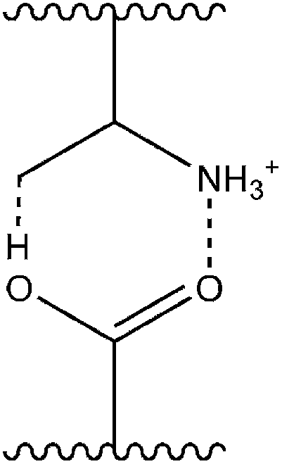Fig. 1 Molecular basis for PAA–PAM interaction at low ionisation.⁸

In solution alone PAA undergoes a conformational change at low pH, switching from an extended chain to a partially coiled system, and this can be studied by inclusion of a fluorescent marker covalently attached along the polymer backbone.^9,10 In this paper we demonstrate how this system can be used as a macromolecular probe to detect IPC formation with PAM via TRAMS, which analyses the rotation of the polymer chain (via the bound fluorescent marker) in space. By comparing parallel and perpendicular polarised light intensities from direct fluorescent excitation TRAMS generates the decay of anisotropy r(t) (eqn (1)). Providing the fluorophore is covalently bound to the polymer backbone this directly measures the segmental motion of the polymer in space.^11,12

r(t) = (I_∥(t) − I_⊥(t))/(I_∥(t) + 2I_⊥(t)) (1)

As samples are excited by polarised light they decay along the same orientation as the incidental light beam. However, this orientation changes continuously due to the molecular motion of the polymer backbone. Provided that this motion is within the excited state lifetime (τ_f) of the fluorophore undergoing a simple relaxation mechanism and it is homogenously distributed along the polymer chain, the anisotropy can be modelled using τ_c, the correlation time, to give the segmental mobility of the polymer backbone. In this equation r_∞ represents the background anisotropy of the system.

r(t) = r_∞ + r₀exp(−t/τ_c) (2)

In complex systems analysis remains possible via combining double (or triple) exponential functions, depending on the appropriateness of the sample. To our knowledge the only previous study of the effect IPC formation has on fluorescence time resolved anisotropy of PAA is work carried out by Heyward and Ghiggino on the interaction of labelled PAA with poly(ethylene oxide)¹³ although long relaxation times due to the formation of rigid complexes have also been observed in solutions of poly(methacrylic acid) and poly(ethylene oxide).¹⁴ Neither of these studies have examined low concentration systems where the probe is in a higher concentration than the binding analyte.

Polymers 1–4 were synthesised via a free radical polymerisation with 4,4′-azobis(4-cyanovaleric acid) (ACVA) as shown in Table 1 and the molar mass data are presented in Table 2. For full experimental conditions see ESI.† Fluorescence anisotropy of labelled polymers yielded a correlation time directly attributable to the polymer backbone segmental mobility. In this way the ‘smart’ or ‘stimuli responsive’ nature of PAA in response to pH can be contrasted to the inert nature of PAM. Dilute solutions of PAA* show a decrease in the correlation time (fitted using eqn (2)) from 6 to 2 nanoseconds in response to pH, whilst PAM* shows no such decrease with τ_c remaining at approx. 1.5 ns as the polymer had no pK_a in the observed region (Fig. 2). Additionally the segmental mobility of these polymers (samples fixed at pH 5) were inversely proportional to temperature (Fig. 3), with neither PAA or PAM demonstrating a lower critical solution temperature or other macromolecular response or state change to temperature change beyond increased motion at higher temperatures. Full details of all fits are contained in the ESI.†

Table 1 Molar ratios of polymers 1–4, *denotes presence of label ACE

	Polymer	Monomer^a	ACVA	ACE
a Monomer refers to AA or AM depending on polymer desired.
1	PAA	100	1.00	—
2	PAA*	100	0.87	0.10
3	PAM	100	1.00	—
4	PAM*	100	1.00	0.10

---

Table 2 Molecular weight of polymers 1–4 determined by GPC

	M n	M w	M z	Đ M
1	58 000	112 550	186 450	1.9
2	42 150	64 900	90 000	1.5
3	9650	47 650	112 850	4.9
4	2000	6450	12 400	3.2

---

Fig. 2 τ _c of PAA* (black dots = polymer 2, avg. χ² 1.10) and PAM* (clear dots = 4, avg. χ² 1.05) with varying pH (0.40 mg ml⁻¹).

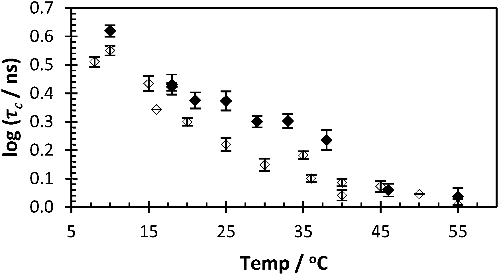Fig. 3 τ _c of PAA* (black dots = 2, avg. χ² 1.13) and PAM* (clear dots = 4, avg. χ² 1.06) with varying temperature (pH 5, 0.40 mg ml⁻¹).

When PAA and PAM are mixed at low pH they interact via repetitive hydrogen bonding across the chain lengths. Upon mixing of polymer 2 with polymer 3 below pH 2.5 the emission spectra showed an increase in fluorescent intensity although there was no change to the steady state profile wavelengths (Fig. 4).

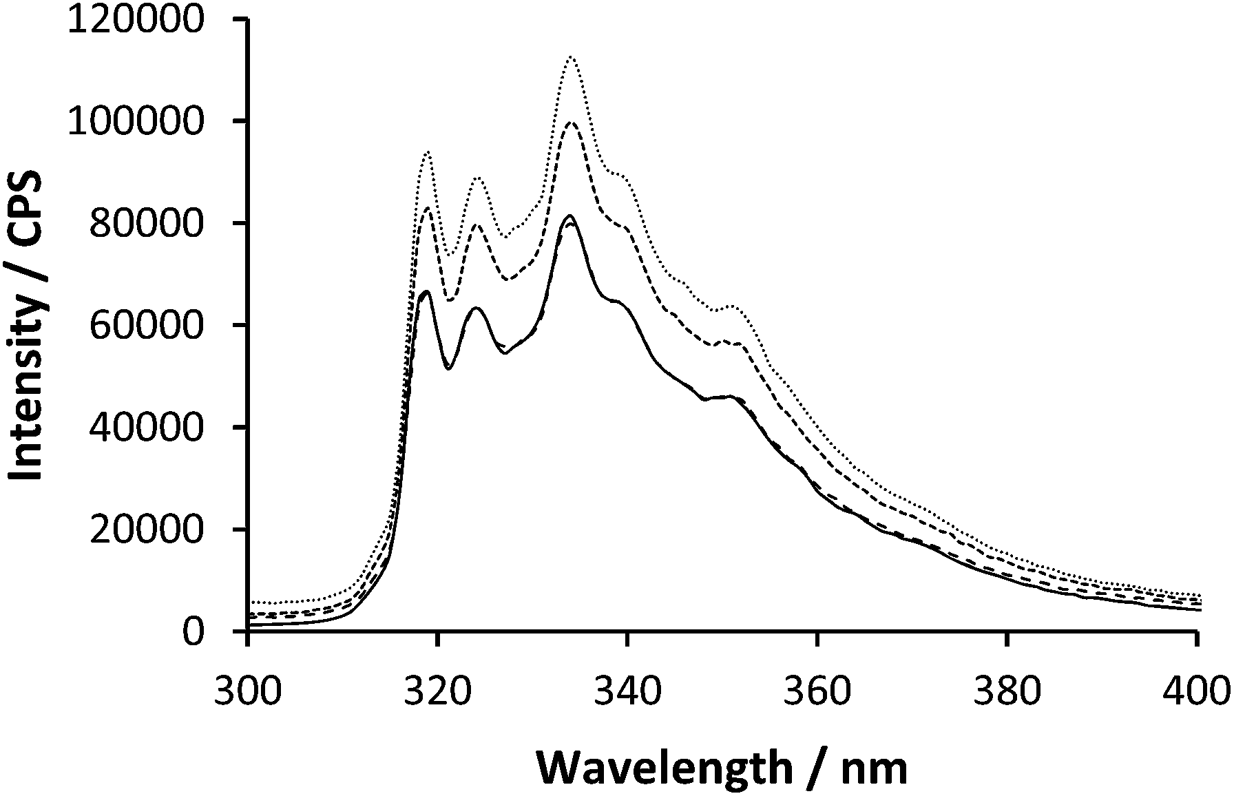Fig. 4 Emission spectra of polymer 2 (0.27 mg ml⁻¹) excited at 295 nm with varying polymer 3 concentration (0.00, 0.08, 0.16 & 0.40 mg ml⁻¹).

This increase was accompanied with increasing light scattering caused by the aggregated polymer particles. Analysis of the fluorescence decay shows no change to the overall lifetime of the fluorophore excited state, although there is increased light scattering from the incidental light beam (see ESI†), suggesting the fluorescence intensity increase is not due to quenching by solvent. Additionally no new peaks were observed in the absorbance of the samples upon mixing (see ESI†) although band broadening did occur.

Time resolved anisotropy measurements respond much more clearly to complex formation. Typically the raw anisotropic signal shows the anisotropy of the sample decaying to zero over a period of time following the initial pulse, however the formation of the IPC adds a slow component to this system (Fig. 5). The same effect was seen when PAM* (polymer 4) was exposed to PAA (polymer 1) (Fig. 6). The increase in residual anisotropy with restricted rotation was not unprecedented,¹⁵ although in previous work on this subject Heyward described the situation of incomplete complexation as giving an undesirable fit, as at low PAM concentrations not all PAA* chains will be engaged in IPC formation.¹³

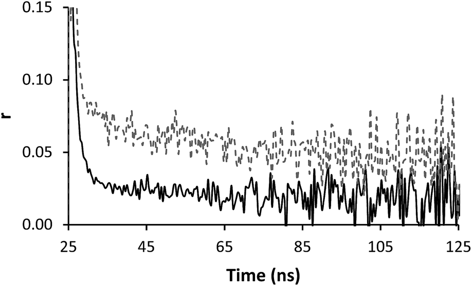Fig. 5 Anisotropy profiles of polymer 2 (solid line) in solution (0.32 mg ml⁻¹) alone and mixed with polymer 3 (dashed line) (0.24 mg ml⁻¹) at pH 2.

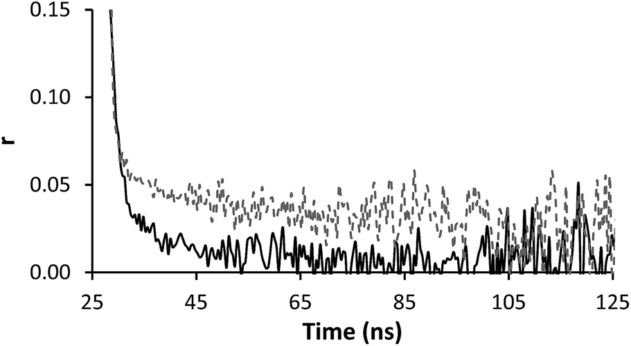Fig. 6 Anisotropy profile of polymer 4 (solid line, 0.13 mg ml⁻¹) alone and mixed with polymer 1 (dashed line, 0.13 mg ml⁻¹) solution at pH 2.

This situation can be adequately studied using a double exponential fit, as shown in eqn (3).

r(t) = A exp(−t/τ_c1) + B exp(−t/τ_c2) (3)

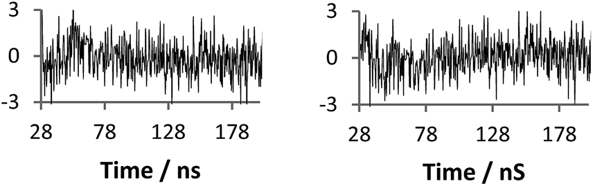
The term r_∞ has been discounted in this equation as it is no longer possible to measure the background anisotropy when the system does not decay to zero during the lifetime of the measurement. Whilst this could be potentially accommodated by the use of a label with a longer excited state lifetime, by fixing the term r_∞ to zero (ensuring that at time t = ∞, r = 0) it is possible to achieve good fits utilising eqn (3) (Fig. 7). Fitting the data to eqn (3) rather than eqn (2) improves the accuracy of the fit (as shown by the residual standard deviations of the fit (Fig. 8)) and allows for differentiation to be made between polymers engaged in IPC formation and those free in solution as τ_c (calculated viaeqn (4)) rises from 12 ns to 180 ns.

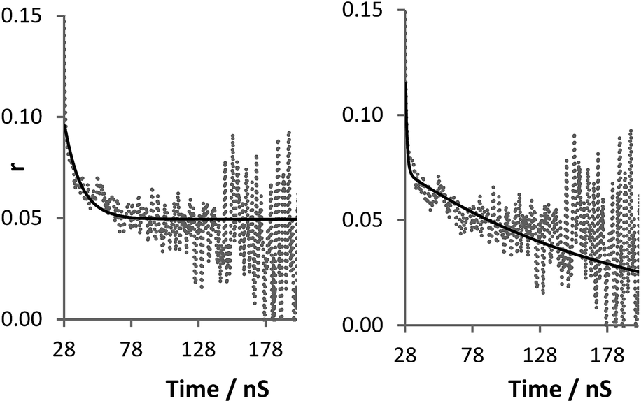Fig. 7 Raw anisotropy data of a polymer 2 + 3 mixture at pH 2 (dashed line), with single exponential fits (solid line) left: eqn (2) (τ_c 12 ns), right: eqn (3) (τ_c 180 ns).

Fig. 8 Residuals (standard deviations) of fits given from Fig. 7 (left eqn (2)χ² 1.35, right eqn (3)χ² 1.12).

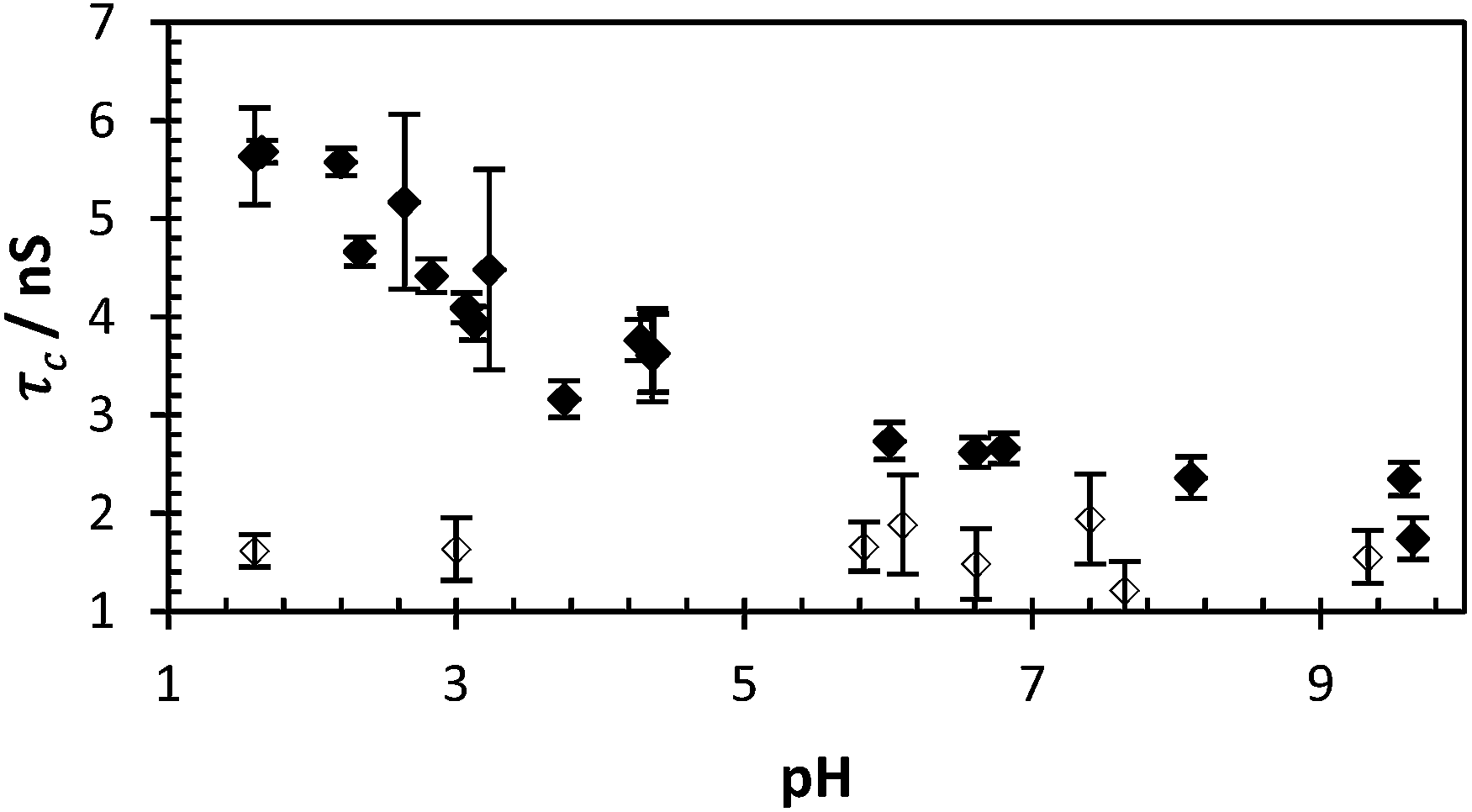
By fixing the term A and τ_c1 to fixed values, τ_c2 (and therefore τ_c) increases in response to IPC formation. Utilising eqn (3) allows for immediate differentiation to be made between samples bound in an IPC and those still dissolved in aqueous solution. In this respect τ_c becomes indicative of the PAA probe's restriction, responding dramatically to the presence of IPC formation. The optimal values for τ_c1 and A were found to be 1.2 ns and 0.0423 respectively. As IPC formation between PAA and PAM is a pH dependent phenomenon the effectiveness of this technique can be demonstrated by comparing a 1 : 1 mixture of polymers 2 and 3 across an entire pH range (Fig. 9). Below pH 2.5, as an IPC forms, and from pH 1–2 the observed correlation time of the ACE fluorophore rises to 180 ns (with an average std. dev. of 6 ns). These results fall into agreement with previous assertions that the critical pH above which IPC will not form for PAA and PAM is approx. 2.3–2.9.⁵

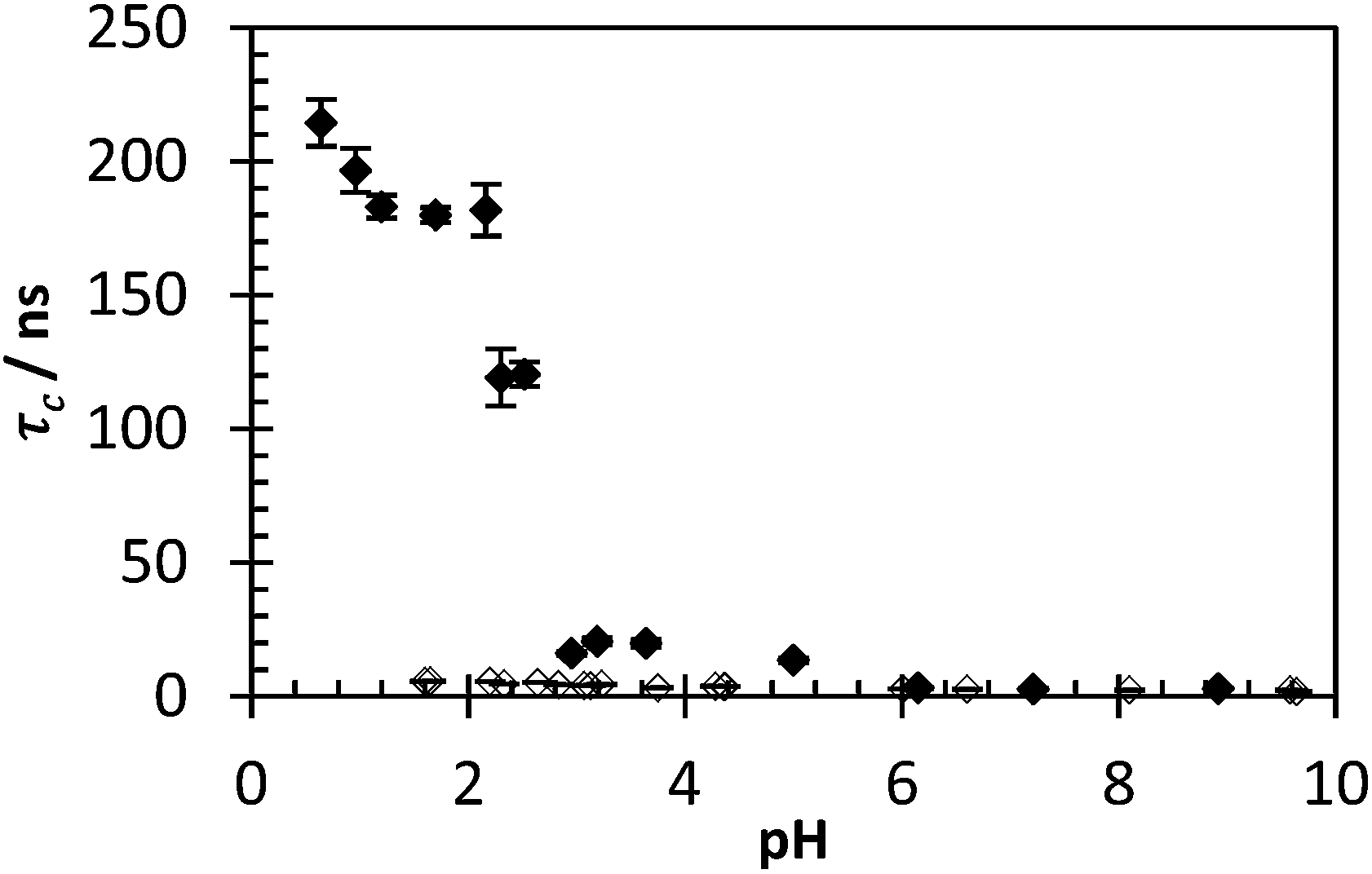Fig. 9 τ _c of polymer 2 with (black dots) and without (clear dots) presence of polymer 3 varying pH. Data fitted using eqn (3) (avg. χ² 1.16, 0.95–1.47).

The distinct response of the anisotropy to IPC formation below pH 3 shows this is an extremely sensitive technique, one that has clear potential as a method of detection for low concentration samples. To this end a series of tests were carried out with the PAA concentration set at 0.2 mg ml⁻¹ (200 ppm), the pH adjusted to 2 and the concentration of PAM varied. As the concentration of PAM (and therefore the level of IPC formation) drops τ_c diminishes revealing a more ‘normal’ anisotropic profile (see ESI† for response profile and residuals), which can be fitted by eqn (3).

(Fig. 10). When the correlation time is calculated a concentration gradient was seen from 0–80 ppm, reaching a peak correlation time at a concentration that is less than half of the concentration of the probe polymer (Fig. 11). This fixed concentration of PAA* was sensitive to levels of PAM over a hundred times more dilute than the probe polymer, and at extremely low PAA* : PAM ratios the calculated correlation time using this measurement showed a smooth decrease in conjunction to PAM concentration. In contrast with Heyward's previous work in this area, considering the concentration of fluorescence PAA probe, the PEO concentration are equivalent to the PAM concentration of Fig. 11 at 200 ppm, a direct 1 : 1 mixing as opposed to a low concentration sensor.¹³

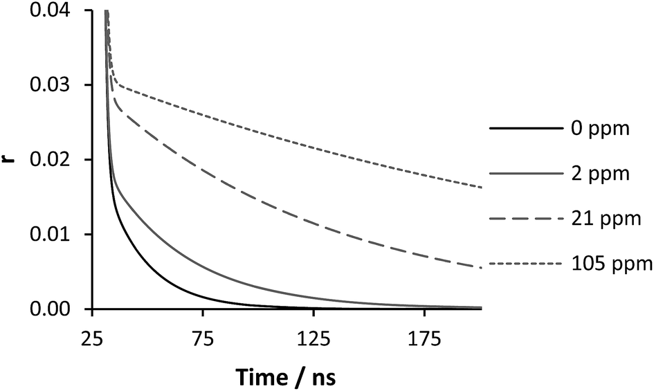Fig. 10 Eqn (3) fitted anisotropy decay of polymer 2 (200 ppm) with varying polymer 3 concentration at pH 2. For full fitting data see Fig. SM3 in ESI.†

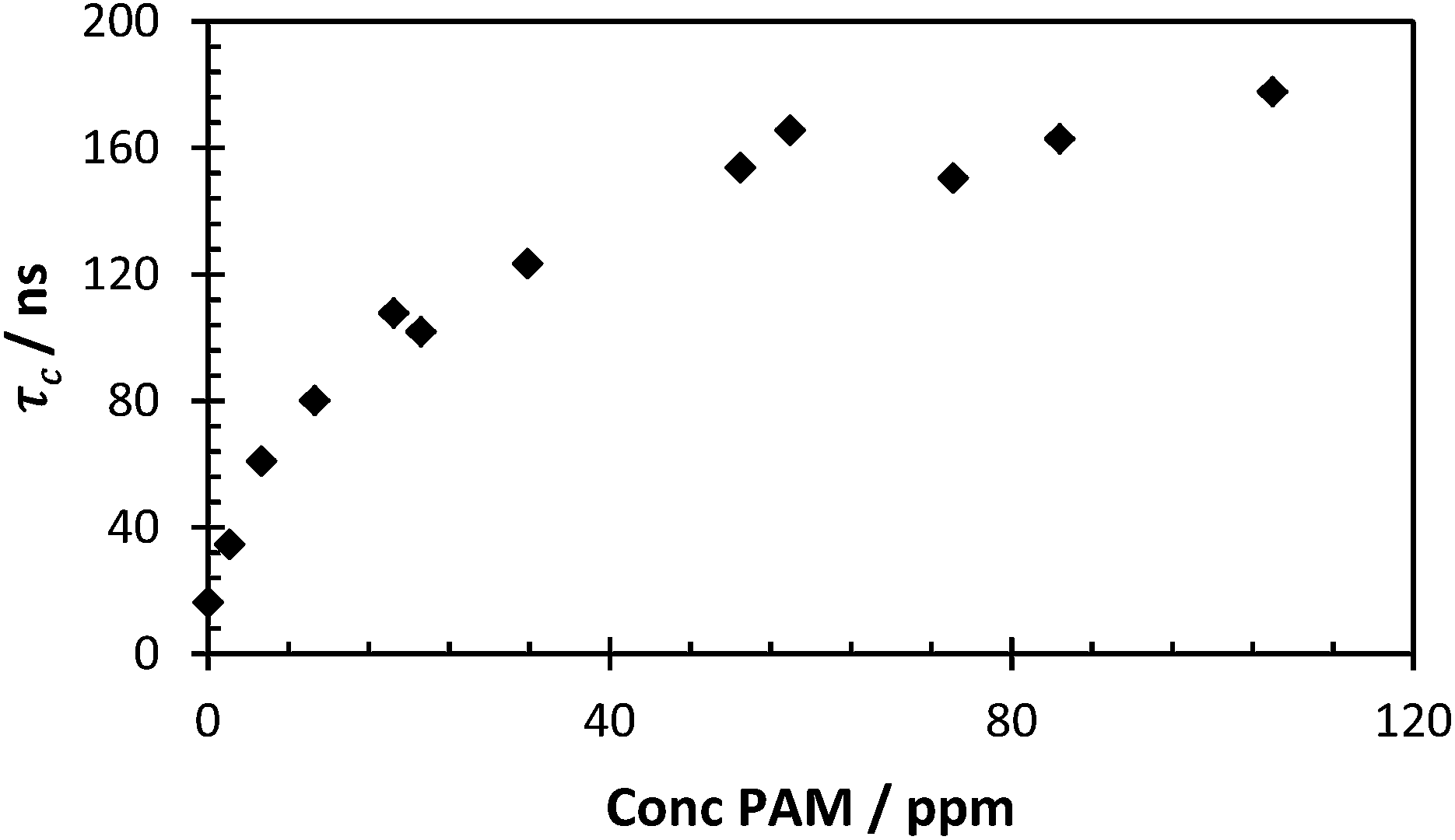Fig. 11 τ _c of polymer 2 (200 ppm) with varying polymer 3 concentration at pH 2 (avg. χ² 1.05, 0.96–1.12).

Conclusions

It is possible to detect the formation of interpolymer complexes between poly(acrylic acid) and poly(acrylamide) at low pH via fluorescence time resolved anisotropy of a covalently attached fluorescent marker. The restricted segmental mobility of these polymers results in a dramatic increase to the correlation time of these samples, an increase that scales appropriately with increasing concentration. As the rise in τ_c is due to repeated hydrogen bonding interactions between polymers this method could be utilised in the further study of many different systems of interpolymer complexation and further work is underway to test the viability of this system in industrial wastewater processes.

Acknowledgements

We thank Professor Mark Geoghegan, University of Sheffield, for his advice on the fitting process. Funding for the research was kindly provided by the Engineering and Physical Sciences Research Council (EPSRC).

Notes and references

1. B. Bolto and J. Gregory, Water Res., 2007, 41, 2301–2324.
2. R. D. Lentz, R. E. Sojka and J. A. Foerster, J. Environ. Qual., 1996, 25, 1015–1024.
3. O. V. Klenina and E. G. Fain, Polym. Sci. U.S.S.R., 1981, 23, 1439–1446.
4. D. J. Eustace, D. B. Siano and E. N. Drake, J. Appl. Polym. Sci., 1988, 35, 707–716.
5. G. A. Mun, Z. S. Nurkeeva, V. V. Khutoryanskiy, G. S. Sarybayeva and A. V. Dubolazov, Eur. Polym. J., 2003, 39, 1687–1691.
6. G. Staikos, K. Karayanni and Y. Mylonas, Macromol. Chem. Phys., 1997, 198, 2905–2915.
7. L. Deng, C. Wang, Z.-C. Li and D. Liang, Macromolecules, 2010, 43, 3004–3010.
8. F. O. Garces, K. Sivadasan, P. Somasundaran and N. J. Turro, Macromolecules, 1994, 27, 272–278.
9. N. Flint, R. Haywood, I. Soutar and L. Swanson, J. Fluoresc., 1998, 8, 327–334.
10. J. R. Ebdon, B. J. Hunt, D. M. Lucas, I. Soutar, L. Swanson and A. R. Lane, Can. J. Chem., 1995, 73, 1982–1994.
11. I. Soutar, L. Swanson, R. E. Imhof and G. Rumbles, Macromolecules, 1992, 25, 4399–4405.
12. I. Soutar and L. Swanson, Macromolecules, 1994, 27, 4304–4311.
13. J. J. Heyward and K. P. Ghiggino, Macromolecules, 1989, 22, 1159–1165.
14. I. Soutar and L. Swanson, Macromolecules, 1990, 23, 5170–5172.
15. J. S. Lee, R. B. M. Koehorst, H. van Amerongen and J. Feijen, J. Phys. Chem. B, 2011, 115, 13162–13167.

---

Footnote

† Electronic supplementary information (ESI) available: Full experimental and synthetic details. See DOI: 10.1039/c4ra07263d

---