Molecular dynamics simulations of the lyotropic reverse hexagonal (HII) of Guerbet branched-chain β-D-glucoside†
Hockseng
Nguan
ab,
Sara
Ahmadi
a and
Rauzah
Hashim
*a
aChemistry Department, Faculty of Science, University of Malaya, 50603 Kuala Lumpur, Malaysia. E-mail: rauzah@um.edu.my
bKavli Institute of Theoretical Physics China, Chinese Academy of Sciences, Beijing 100190, China
First published on 18th October 2013
Abstract
Through atomistic molecular dynamic simulations using a GROMOS53a6 force field for the carbohydrate, we studied the lyotropic reverse hexagonal phase HII from a glycolipid, namely the Guerbet branched-chain β-D-glucoside, at 14% and 22% water concentrations. Our simulations showed that at low water concentration (14%) the sugar head group overlapped extensively and protruded into the water channel. In contrast, in the 22% concentration system a water column free from the sugar headgroup (‘free’ water) was formed as expected for the system close to the limit of maximum hydration. In both concentrations, we found anomalous water diffusion in the xy-plane, i.e. the two-dimensional space confined by the surface of the cylinder. On the other hand, along the z-axis, the water diffusion obeyed the Einstein relation for the 22% system, while for the 14% system it was slightly anomalous. For the 22% system, the diffusion along the z-axis of the ‘free’ water obeyed the Einstein relation, while that of the ‘bound’ water is slightly anomalous. The xy-plane displacement of the ‘bound’ water was higher than that for the ‘free’ water at times longer than 200 ps, as a consequence of the exchange of water molecules between the two regions. Based on our findings, we proposed an alternative explanation to the observed spatial heterogeneity in the HII phase from probe diffusion by Penaloza et al. (Phys. Chem. Chem. Phys., 2012, 14(15), 5247–5250). We found the extent of contact with water was different at different oxygen atoms within the sugar ring. Generally, a higher probability of hydrogen bonding but a shorter lifetime was found in 22% water compared to the case of 14% water. Finally, we examined the extension and compression of the alkyl chain of a columnar.
I. Introduction
Glycolipids are amphiphiles, which consist of a hydrophilic part that is made of sugar while hydrocarbon chains form the hydrophobic part. They give rise to a variety of liquid crystal phases both in dry and hydrated environments.1,2 In nature, glycolipids exist in the cell membrane, albeit in a relatively small amount compared to phospholipids, which form the major components.3–5 To supplement the scarcity of natural products, a number of nature-like synthetic glycolipids have been prepared and their liquid crystal behaviours have been studied both experimentally6–11 and theoretically.12–14 Depending on the balance between the attractive forces in the headgroup region and the repulsive forces between the lipid tails, a variety of self-organized structures may be observed from the simple one-dimensional (1-D) lamellar (Lα) phases to two-dimensional (2-D) hexagonal (H) phases to the more complex three-dimensional (3D) cubic (Q) phases. Modifying the balance between these forces by changes in temperature or hydration may lead to transitions between these different phases.Among the family members of glycolipids, alkyl glycosides are interesting both biologically15 and industrially.16 These sugar-based surfactants are biodegradable, nontoxic, and may be synthesized from cheap renewable resources. They are interesting as substitutes for many ionic commercial surfactants, which are harmful to the environment.17 A typical nature-like synthetic glycolipid is the Guerbet branched-chain β-D-glucoside, which has been studied extensively and reviewed in ref. 1. This family of glycosides contains a sugar headgroup connected via a glycosidic linkage to two asymmetric chains which differ by two methylene units. Moreover, the two chains branch at the β-carbon position which is also chiral. The Guerbet glycoside series can be viewed as a Guerbet sugar, an addition to other Guerbet materials including alcohol, ester, and acid, all of which have many industrial applications.18,19 These Guerbet glycosides can be found in a variety of liquid crystalline phases, including the reversed hexagonal (HII) at some water concentrations.2
In general, the lyotropic HII phase consists of glycolipid aggregates in column structures which are arranged further to form a hexagonal lattice. In a reverse hexagonal phase (HII), each column has a core filled by water molecules forming a water channel. These water molecules are surrounded by a monolayer of amphiphilic glycolipid molecules with the hydrophilic part pointing inward into the water channel while their hydrophobic chains point outward. The HII phase is stable in the excess water environment and can be dispersed in water to form nanoparticles.20–25 These nanoparticles are potentially useful for applications in controlled release drug delivery. Besides, the ability to transition from a lamellar to an inverted hexagonal phase is of particular importance in biological systems.26 For example, the appearance of a reverse hexagonal (HII) phase occurs because of a partial dehydration of microsomal membranes,27 as shown from isotropic 31P-NMR signals of isolated microsomes of liver cells.28–30 In these studies, the microsomes have a high tendency to form an HII phase. It was found that the addition of fusogenic agents such as unsaturated fatty acids to phospholipid bilayers, or to natural membranes, tended to induce the formation of an HII phase as well as promote fusion. The HII phase was also found in the formation of cationic liposome–DNA complexes (lipoplexes),31 which are widely studied for their useful application in intercellular gene delivery.32,33 Although the HII phase is the most common of non-lamellar phases in biological lipid systems34 the theoretical basis for understanding water and guest molecules behaviour has been scarcely studied compared to lamellar systems.
Atomistic molecular dynamics (MD) simulations are a very useful theoretical tool in the understanding of liquid crystal behaviour from detailed interactions at the atomic level. This method has been successfully applied to lamellar and non-lamellar self-organized membrane systems.35 Possibly, the earliest atomistic MD simulation of HII was by Bandyopadhyay et al.,36 where a system of two columnar hydrated sodium dodecylsulphates was simulated for a production stage of 260 ps, which gave the structure of a distorted hexagonal symmetry consistent with the experimental results by Leigh et al.37 On the other hand, a series of MD simulations of the phase transition into the HII phase has also been investigated,38–40 which helps provide insight into the membrane fusion of biological cells. More recently, a 10 ns MD simulation study focused on the water channel of an HII of glyceryl monooleate (GMO) was done by Kolev et al.41 There, only the water molecules were allowed to move and were confined in the channel surrounded by GMO, which restrained any movement.
In this work, we modelled the lyotropic liquid crystals of the (2′n-octyl-n-dodecyl)-β-D-glucopyranoside (C8C12β-D-Glc) in the HII phase.2,42 In the simulation, two different water concentrations (14% and 22% of the total weight of the each system) were chosen and the lattice parameters used in the study were taken from small-angle X-ray experiments.42 The simulation measured various physical properties of the systems such as the movement of the confined water molecules and the hydrogen bonding between the water and the sugar head of C8C12β-D-Glc. In addition, the hydration shells of the sugar head at two different concentrations were analysed. The results of the analysis help in understanding the behaviour of water confined by cylindrical non-ionic surfaces. The simulation also analysed the chain elongation related to the packing frustration of the HII. In the following section, we shall describe the preparation and modelling of the initial structure for the simulation of the reverse hexagonal phase.
II. Preparing and modelling of the reverse hexagonal phase
We began by constructing a full atomistic model of C8C12β-D-Glc (see Fig. 1a) using the modelling software package Avogadro,43 followed by a brief energy minimization using molecular mechanics with a MMFF94 forcefield.44 Subsequently, in the pre-constructed atomistic model of C8C12β-D-Glc, all hydrogen atoms were removed except the four hydrogen atoms from the hydroxyl groups within the sugar unit. Hence a united atom model was built (see Fig. 1b), whose carbohydrate force field was obtained from GROMOS53a6.45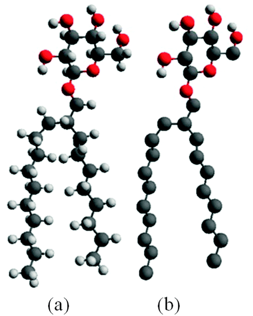 | ||
| Fig. 1 (a) Fully atomistic model of (2′n-octyl-n-dodecyl)-β-D-glucopyranoside (C8C12β-D-Glc); (b) the united atom model of C8C12β-D-Glc. | ||
In order to construct the initial configuration of the reverse hexagonal phase using the united atom model of C8C12β-D-Glc the following steps were applied. Firstly, the C8C12β-D-Glc was replicated into a number of copies. These were arranged into a disc with a hole in the middle. Ten of these disc aggregates were stacked to form a column. The column was replicated and arranged into a hexagonal lattice (see Fig. 2(a)). Separately, a configuration of randomly distributed water molecules residing in a rectangular box was generated using the genbox utilities software in the GROMACS MD simulation package.46,47 The length of the rectangular box along its long axis was determined according to the length of the column. In addition, the surface area perpendicular to its long axis was made small enough for the box to be inserted into the hollow space of the column. The water box was later replicated six times and each of these was inserted into the hollow space of the column. Subsequently, this configuration was used as the initial structure of our HII simulation as shown in Fig. 2(b), where the yellow dotted lines indicate the boundaries of the periodic box. Our approach in setting the periodic boundary condition is similar to the one used by Bandyopadhyay et al.36 Each column was assigned to a number in order to keep track of any changes in its appearance.
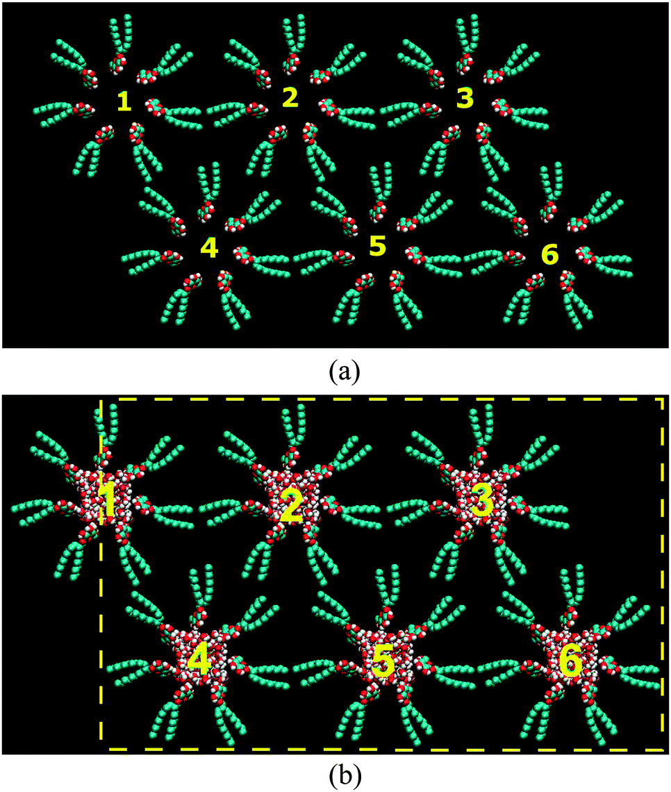 | ||
| Fig. 2 (a) Six columnars of C8C12β-D-Glc arranged in a hexagonal lattice. (b) The initial configuration for the MD simulation, where the yellow lines indicate the periodic boundary. | ||
In the construction of a single column, the size of the hole depends on how close the nearby C8C12β-D-Glc molecules are to each other when arranged into a column structure. It should be made large enough to accommodate the targeted number of water molecules, i.e. 1746 and 3023 for the 14% and 22% water systems, respectively. This made up a total number of atoms of 20![[thin space (1/6-em)]](https://www.rsc.org/images/entities/char_2009.gif) 358 and 24189 for the two systems, respectively. In the simulation, the starting structure can affect the time the simulation takes to achieve equilibrium. The closer the initial hexagonal structure is to the experimental one, the faster the simulation will reach the equilibrium state that agrees with the real system. However, compared to the flat membrane-like bilayer model system, it is relatively hard to construct an initial structure of an HII phase that is close to the equilibrium state. Therefore, we tested a number of different initial structures, each of which differed in terms of the radius and length of the hollow space, hence the size of the rectangular box of water molecules. These initial structures were first energy minimized using the steepest descent method to remove bad contacts between molecules; and subsequently followed by MD simulations with constant pressure (NPT) performed for 5 ns at a temperature T = 298 K. From this series of simulations, the system whose result that gave the average lattice parameter closest to the experimentally measured value after 5 ns of simulation was chosen. Amongst the configurations generated from the chosen simulation system, we further selected the frame, which most closely matched the experimentally measured lattice parameters. This selected frame became the starting configuration for a further MD simulation of 50 ns. In this work we focused on two systems of HII formed by C8C12β-D-Glc with two different water contents of 14% and 22%, respectively. Here, water molecules were modelled as in the simple point charge (SPC) model.48
358 and 24189 for the two systems, respectively. In the simulation, the starting structure can affect the time the simulation takes to achieve equilibrium. The closer the initial hexagonal structure is to the experimental one, the faster the simulation will reach the equilibrium state that agrees with the real system. However, compared to the flat membrane-like bilayer model system, it is relatively hard to construct an initial structure of an HII phase that is close to the equilibrium state. Therefore, we tested a number of different initial structures, each of which differed in terms of the radius and length of the hollow space, hence the size of the rectangular box of water molecules. These initial structures were first energy minimized using the steepest descent method to remove bad contacts between molecules; and subsequently followed by MD simulations with constant pressure (NPT) performed for 5 ns at a temperature T = 298 K. From this series of simulations, the system whose result that gave the average lattice parameter closest to the experimentally measured value after 5 ns of simulation was chosen. Amongst the configurations generated from the chosen simulation system, we further selected the frame, which most closely matched the experimentally measured lattice parameters. This selected frame became the starting configuration for a further MD simulation of 50 ns. In this work we focused on two systems of HII formed by C8C12β-D-Glc with two different water contents of 14% and 22%, respectively. Here, water molecules were modelled as in the simple point charge (SPC) model.48
For the two systems, energy minimisation was performed on each of their initial configurations, followed by a constant pressure simulation of 50 ns, where the first 10 ns was taken as the equilibration stage while the last 40 ns was considered as the production stage. All the simulations applied the period boundary condition and leap-frog algorithm for the integration of the Newtonian equations of motion with a time-step of 2 fs. In addition, a LINCS algorithm was used to fix the bond lengths involving the hydrogen atoms. The particle mesh Ewald (PME) approach was employed to calculate the electrostatic interactions with a cut-off of 12 Å. The cut-off of 12 Å was applied for the non-bonded interactions calculation. The temperature was controlled by a Nose–Hoover thermostat, while the isotropic pressure was applied using Parrinello–Rahman pressure coupling.
III. Results and discussion
A. Structure of the reverse hexagonal HII
The final configurations from the simulations of the two systems with different concentrations are given in Fig. 3(a) and (b), which show stable hexagonal arrangements, with box dimensions of 11.8 nm × 6.9 nm × 4.8 nm and 11.8 nm × 6.9 nm × 4.8 nm, respectively. The stability of the simulation systems over the course of the simulation was checked according the profile of the lattice parameter (i.e. average distance between two cylinders) and radial density profile over time (see Fig. S1 and S2 in the ESI†). Here, the distance between two cylinders is defined as a two dimensional (i.e. X and Y axes) distance between the centres of mass of the two water columns (the lattice parameter). For each time frame, the lattice parameter between two neighbouring cylinders is evaluated from all the possible pairs of neighbours from the six cylinders. The time-averaged lattice parameters are tabulated in Table 1, which is in relatively good agreement with the experimental measurements.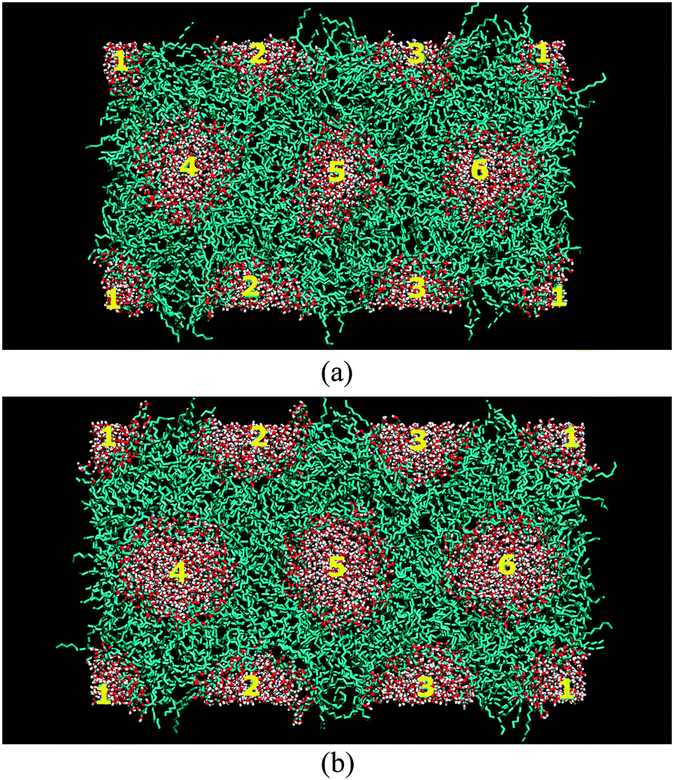 | ||
| Fig. 3 The configurations of the HII phase after 50 ns for the system with (a) 14% water and (b) 22% water. | ||
The lyotropic HII self-assembly of C8C12β-D-Glc has three regions, namely water, the sugar head region and the hydrocarbon chain. Slight overlapping between the regions is expected at the interfaces. Taking advantage of the hexagonal symmetry, we calculated the radial distribution of the mass density with a centre located in the water region of cylinder number 5 (see Fig. 3) as a reference point. The radial density distributions are as displayed in Fig. 4. Extensive overlapping exists in the HII of C8C12β-D-Glc with 14% water concentration (Fig. 4(a)), implying the sugar headgroup penetrates into the water channel. In contrast, the overlapping of sugar and water density profiles is less in the system with 22% water. This suggests at low water concentration, the sugar head is less able to separate from the water region, compared to the case of a higher water concentration where water column free of sugar headgroup is found.
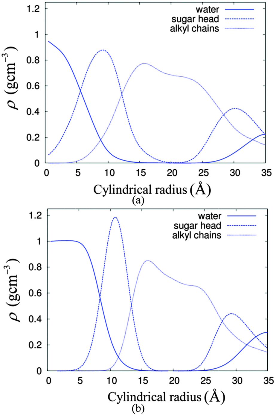 | ||
| Fig. 4 The radial density profiles of the water, sugar head group and alkyl chains for systems of HII with (a) 14% water and (b) 22% water. | ||
Based on these results, we estimated the area per head group, A, using the equation
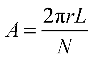 | (1) |
B. Diffusion of water molecules in the water channel of HII
It is well known that the dynamics of water confined in a nanoscale space is different from that of bulk water,52,53 since the interactions between the water molecules and its wall is significant in an overall system. These interactions depend on the type of functional groups on the wall,54,55 which could be stronger in the confined environment than in the bulk.56,57 The famous examples of such conditions are water inside a carbon nanotube58,59 and the aquaporin.60–62 One of the direct consequences of the water–wall interaction is the flow properties of the confined water. Recent experiment has found heterogeneity in the diffusion of the water regions within the HII system formed by the hexaethylene glycol, a non-ionic surfactant.63 Since C8C12β-D-Glc is also a non-ionic surfactant, we believe the behaviour of water in its HII phase resembles that of a hydrophilic nano-channel, similar to the case of hexaethylene glycol referred to previously.63 The experimental results showed that in the reverse hexagonal phase, HII, there are two types of diffusions, namely ordinary Einstein's diffusion (due to the thermal effect) and an anomalous diffusion which may be due to the restricted motion. The Einstein diffusion phenomena can be described by the Einstein relation, 〈Δr2〉 ∼ t, where 〈Δr2〉 is the mean square displacement of particles and t is time. This relationship can be written into Einstein's diffusion equation,| 〈Δr2〉 = 2dDt, | (2) |
| 〈Δr2〉 ∼ tα | (3) |
We investigated the diffusion behaviour of the two simulated systems by calculating the mean square displacement of the water molecules. The displacement along the columnar axis, i.e. the z-axis, was calculated separately from the displacement in the plane perpendicular to the columnar axis, i.e. the xy-plane. These calculations were performed using the utility program g_msd in the GROMACS software package. The log–log plots of the mean square displacement as a function of time are given in Fig. 5.
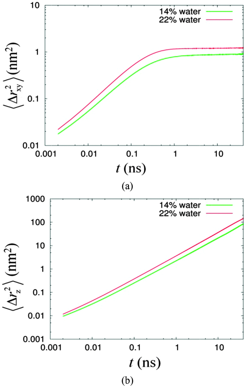 | ||
| Fig. 5 The mean square displacements of water versus time (a) in the xy-plane and (b) in the z direction for 14% (green line) and 22% (red line) systems. | ||
Fig. 5 shows the mobilities of confined water in the z direction and the xy-plane are higher for the system of higher water concentration. Fig. 5(a) shows the diffusion of water in the xy direction is anomalous, with the exponent α equal to 0.76 and 0.81 for system of 14% water and 22% water, respectively (see Table 2) for the region less than 100 ps. These results were obtained by a linear regression analysis, where values of α were calculated from the slope of the linear fitting lines. We observe that the time scale for the anomalous diffusion is independent of the water concentration. Beyond 100 ps, the MSD (mean square displacement) of water levels off at different limiting values for different concentrations. Moreover, the limiting MSD for the 22% system is larger compared to that for the lower concentration system. In the former, the motion of water is less confined since it has a bigger water channel. In addition, upon close inspection of these long time scale diffusions, we found that these are not completely flat. Instead, both have significantly measurable gradients (see Table 2). In contrast, the diffusion along the z direction in Fig. 5(b) for the 22% system conforms to the Einstein's relation, while for the less concentrated system 14% water, this deviates slightly from the Einstein's relation (see Table 2). Ignoring the slight deviation, and assuming a normal behaviour for both, the values of the diffusion coefficients for the 14% and 22% systems are 1.0 (±0.1) × 10−5 cm2 s−1 and 1.8 (±0.1) × 1−5 cm2 s−1, respectively. Compared to the diffusion of SPC water measured in a bulk system, which is 4.20 (±0.01) × 10−5 cm2 s−1,64 these simulated values are 4–2 times slower.
| System | Diffusion in the xy-plane | Diffusion in the z-axis | ||
|---|---|---|---|---|
| α when t ≤ 100 ps | α when t ≥ 5 ns | α over the production time | D (10−5 cm2 s−1) | |
| 14% water | 0.76 | 0.02 | 0.98 | 1.1 ± 0.1 |
| 22% water | 0.81 | 0.01 | 1.00 | 1.8 ± 0.1 |
From the radial density distribution (see Fig. 4), for the 14% water system, most of the water molecules are ‘bound’ to the sugar headgroups, but at the higher water concentration (22% water system), there are both ‘free’ water molecules, i.e. those which are in the sugar free region, and a relatively small amount of ‘bound’ water. Thus, it is interesting to characterise further the dynamical behaviour of the 22% water system, since water molecules from these two regions may travel (and exchange) with each other. Over a long period of time each water molecule should have travelled and exchanged between these two regions frequently. We investigated diffusion behaviours of water molecules from these two regions based on the water column number 5, which contains 502 water molecules. The ‘free’ and ‘bound’ waters were distinguished using the radial density profile (Fig. 4b), in which the plot of the water density crosses the sugar head density at about 0.83 nm. This radial distance was taken as the boundary separating these two water regions. Over the 50 ns total simulation time, a series of configurations starting from 11 ns, 12 ns to 40 ns, were selected and used as the reference frames of the 10 ns MSD calculations. From each selected configuration, the ‘bound’ and ‘free’ waters were identified and distinguished from each other, using a computer code, which search for the ‘free’ and ‘bound’ waters based on the boundary criterion described above. The different labels were written into the GROMACS index group files of ‘free’ water and ‘bound’ water, respectively. The analysis showed the average percentage of the ‘free’ water is about 65% while that for the ‘bound’ water is 35%. The MSD calculations of ‘free’ and ‘bound’ water based on each respective index group file over 10 ns time were performed, using the g_msd utility program, for over 30 selected time periods and the selected reference configurations. Finally these two sets of MSDs for bound and free waters were averaged and the 10 ns dynamic profiles for both bound and free waters in z-axis and xy-plane are shown in Fig. 6.
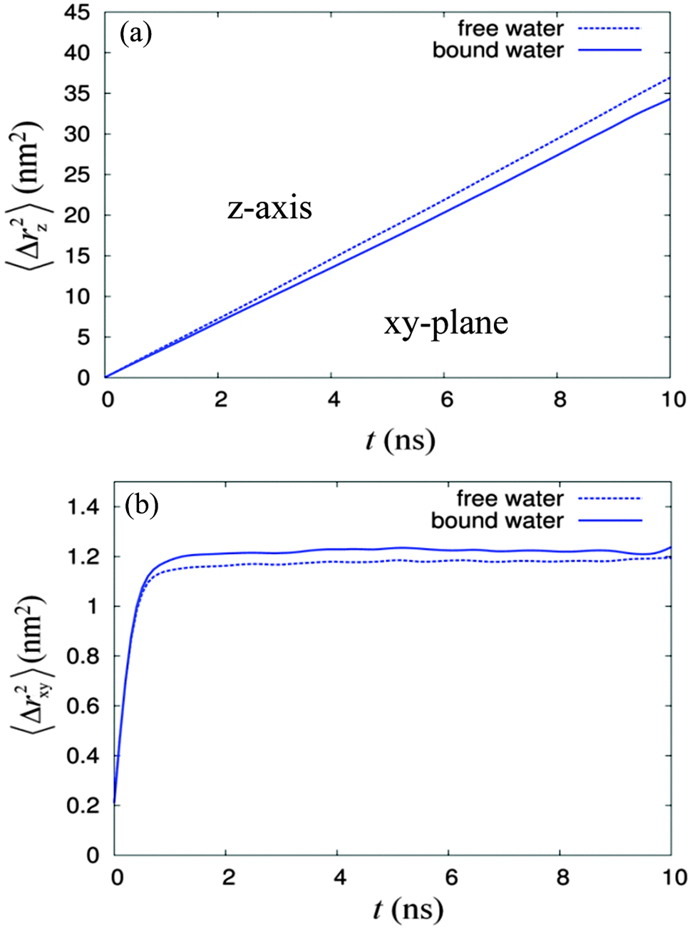 | ||
| Fig. 6 The mean square displacements versus time over 10 ns dynamics for the ‘free’ (dotted line) and ‘bound’ (solid line) waters, where (a) is along the z-axis and (b) is in the xy-plane. | ||
The results show that diffusion of the ‘free’ water in the z-axis is faster compared to that of the ‘bound’ water, as expected. Further analysis on the 〈Δrz2〉 profiles in Fig. 6(a) suggests that the diffusion of the ‘free’ water is normal, while that for the ‘bound’ water is slightly anomalous with the exponent α being equal to 0.99. The diffusion in the xy-plane (see Fig. 6(b)) for both cases follows a power law at time periods less than 100 ps, with the exponent α equal to 0.81, similar to that previously found for the overall water diffusion of 22% system (see Table 2). In this xy-plane, the diffusion of the ‘free’ water is slightly higher than that of the ‘bound’ water during times less than 200 ps, but it is overtaken by the diffusion of the ‘bound’ water after 200 ps; both profiles of the 〈Δrxy2〉 start to saturate after 1 ns. Furthermore, profiles of 〈Δrxy2〉 over time shown that the diffusion of water molecules from the ‘bound’ water region saturated to a higher average displacement in the xy-plane compared to those of ‘free’ water molecules. By comparing two configurations with a time difference of 10 ns, it was found that the average number of water molecules exchanged between the two regions is about 114. Our analysis suggest that in short period of time (i.e. less than 200 ps), the diffusion of ‘bound’ water was slowed down by the sugar head group. As time was increased further, some exchanges happened between the ‘bound’ water and ‘free’ water. These exchanges enhanced the average displacement of water molecules from the ‘bound’ water and at the same time reduced that of the ‘free’ water. Since C8C12β-D-Glc is a non-ionic surfactant and the sugar headgroup is not too different from the glycol moiety of a similar common surfactant hexaethylene glycol (C12E6), the water diffusion phenomena for both should be relatively similar. Therefore our simulation results could offer an alternative detailed explanation for the particle tracking experiment in the HII phase formed by hexaethylene glycol.63 They measured the diffusion of polystyrene (PS) probes using an optical tweezers technique65 in isotropic, reverse hexagonal and lamellar phases at three concentrations: 20%, 50% and 80% of C12E6 respectively. They found that the diffusion of PS in both lamellar and isotropic phases conforms to a normal diffusion pattern, but in the reverse hexagonal phase, both normal diffusion and sub-diffusion behaviour was observed. They explained that the presence of two diffusion phenomena is due to the heterogeneous local environment within the reverse hexagonal structure, i.e. the presence of an isotropic local domain where PS diffusion is normal, and a hexagonal local domain where the PS diffusion is restricted giving the sub-diffusion phenomenon. However, based on our simple simulation model of the reverse hexagonal phase, the diffusion of water in the z-axis along the column is normal but in the xy-plane is sub-diffusion. Since the particle tracking experiment only captured two-dimensional displacements of the PS, the diffusion pattern of the probe in 2D is necessarily sub-diffusion depending on the orientation of the water column with respect to the laboratory Z-axis. Therefore, we believe that the origin of heterogeneity in the local environment is due rather to the existence of the local domains of HII in the measured sample with different columnar orientations. The probe particles inserted during the experiment could have been distributed among these local domains, therefore various diffusion behaviours were observed. To show how the orientation of the columnar axis affects the two-dimensional diffusion pattern, we begin with a three-dimensional mean square displacement of a probe particle in a certain columnar phase, denoted as 〈rXYZ2〉, where XYZ represent the laboratory axes. 〈rXYZ2〉 can be defined as,
| 〈rXYZ2〉 = 〈ΔX2〉 + 〈ΔY2〉 + 〈ΔZ2〉 | (4) |
| 〈rxyz2〉 = 〈Δx2〉 + 〈Δy2〉 + 〈Δz2〉 | (5) |
Here, Δx, Δy and Δz are the displacements according to the columnar axis system. In principle,
| 〈rXYZ2〉 = 〈rxyz2〉. | (6) |
If the z-axis of this column deviates from the Z-axis by an angle θ,
| ΔZ = Δzcosθ | (7) |
In the particle-tracking experiment, the two-dimensional displacement measured is 〈rXY2〉. Consequently,
| 〈rXY2〉 = 〈rXYZ2〉 − 〈ΔZ2〉 = 〈rxyz2〉 − 〈Δz2〉cos2θ. | (8) |
As shown in our simulation, the diffusion of water molecules in the confined xy-plane behaves anomalously, hence the probe particles' diffusion should behave likewise. This implies that
| 〈rxy2〉 = 4Dxytβ and | (9) |
| 〈Δz2〉 = 2Dzt, | (10) |
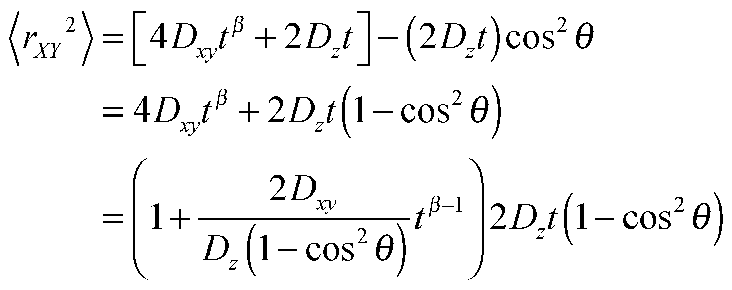 | (11) |
Eqn (11) shows that the particle displacement measurement in two dimensions can deviate from the normal diffusion phenomena depending on the orientation of the columnar axis. One can see that as long as θ ≠ 0, the time-dependent term, 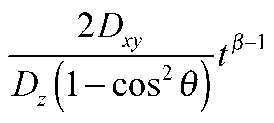 will decrease as time increases. Eventually,
  becomes insignificant, then eqn (11) effectively conforms to Einstein's diffusion relation. Therefore, for long enough times the two-dimensional diffusion in the HII is normal, except when the direction of the z-axis of the column coincides with the laboratory Z axis, i.e. when θ = 0, where anomalous diffusion will be observed. Moreover, when these two axes do not coincide but the time of measurement is long enough, only normal diffusion is observed, such that
| 〈rXY2〉 ≈ 2Dzt(1 − cos2θ) | (12) |
This means the diffusion coefficient measured based on the laboratory reference axes, denoted as Dlab, is effectively related as
| Dlab = Dz(1 − cos2θ)/2, | (13) |
From this analysis, we show that the 2D diffusion pattern observed depends on the columnar orientations with respect to the laboratory axis. In reality, the columns' orientations in the HII phase at thermal equilibrium are not perfectly uniform due to the existence of local domains, which leads to deformations and defects inside the system that can be observed under the polarizing microscope.66 In the experiment, different probe particles inserted might fall into some parts of the columnar phase with different orientations, leading to different diffusion patterns observed. This seems to explain the diffusion phenomena HII of C12E6 given by the experiment.63
C. Interaction between water and the sugar headgroup at different water concentrations
Within the reverse hexagonal phase HII, the water molecules interact extensively with the sugar headgroup at the interface between the water region and the sugar head region. One of the important interactions is the hydrogen bond, which involves the water molecules and the oxygen atoms from the sugar headgroup. These hydrogen bonding interactions can be extracted from the simulations. A hydrogen bond is characterised according to the geometric criteria such that the oxygen to oxygen atom distance must be less than 3.5 Å and the O–H⋯O angle less than 30°.68,69 Based on these criteria and using the g_hbond utilities software in GROMACS, we calculated the time-averaged number of hydrogen bonds per sugar head for each hydroxyl group (donor) and the oxygen atoms (acceptor) on the sugar head itself (see Fig. 7). The results of the calculations for the two water concentrations system are given in Table 3. This shows that for both water concentrations, among the six oxygen atoms acting as hydrogen bonding acceptors on the sugar head, O6 gives the highest number of hydrogen bonds with water molecules, followed by O3, O2, O4, O5 and finally O1. Meanwhile, among the four hydroxyl groups on the sugar head, the highest hydrogen bond number is for the donor O4–H, followed by O3–H, O6–H and O2–H (Table 3). Table 3 also shows that for each site (both for donor and acceptor) the number of hydrogen bonds is higher for a high water system due to the availability of water molecules to participate in the hydrogen bond formation and a larger interface in the system of high water content.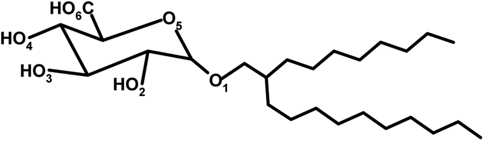 | ||
| Fig. 7 Designation of oxygen atoms on the sugar head for C8C12β-D-Glc. | ||
| Water–sugar hydrogen bond | Average no. of hydrogen bond per sugar head | Hydrogen bond life time (ps) | |||
|---|---|---|---|---|---|
| 14% water | 22% water | 14% water | 22% water | ||
| Acceptor | O1⋯H–Owater | 0.02 | 0.03 | 1.5 | 1.5 |
| Acceptor | O2⋯H–Owater | 0.30 | 0.36 | 30.8 | 18.0 |
| Acceptor | O3⋯H–Owater | 0.44 | 0.50 | 13.1 | 9.4 |
| Acceptor | O4⋯H–Owater | 0.27 | 0.29 | 15.6 | 13.6 |
| Acceptor | O5⋯H–Owater | 0.08 | 0.12 | 8.3 | 5.2 |
| Acceptor | O6⋯H–Owater | 0.57 | 0.69 | 16.7 | 11.9 |
| Donor | O2–H⋯Owater | 0.26 | 0.36 | 53.0 | 38.3 |
| Donor | O3–H⋯Owater | 0.34 | 0.40 | 32.5 | 25.1 |
| Donor | O4–H⋯Owater | 0.46 | 0.50 | 25.9 | 20.5 |
| Donor | O6–H⋯Owater | 0.34 | 0.43 | 39.0 | 31.8 |
The dynamics of the hydrogen bonding interactions between water and sugar head were also investigated. The lifetime of the hydrogen bond was analysed by calculating the autocorrelation function of the hydrogen bond existence, C(τ), defined as
| C(τ) = 〈si(t)si(t + τ)〉, | (14) |
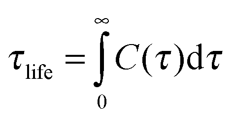 | (15) |
Table 3 gives the results of this analysis and shows that in both systems, the donor hydrogen bond at O2–H⋯Owater has the longest lifetime compared to the other sites. In addition, the hydrogen bond O2⋯H–Owater has the longest lifetime among acceptor oxygens. This indicates that the water molecules are more confined when bonded with the hydroxyl O2–H site compared to when bonded with the other hydroxyl groups. Consequently, water molecules close to the O2 site penetrate deeper into the sugar region and are somewhat trapped. On the other hand, even though the glycosidic oxygen O1 and O5 are located deeper within the sugar structure, their partial charges are less negative than those of O2. Therefore the hydrogen bonds on O1 and O5 are less stable than that of O2. Table 3 also shows that the lifetime of each particular hydrogen bond considered for the system of 14% water, is longer than that of the 22% water system. This is expected since the diffusion of water molecules in smaller size water channels of 14% water is lower than in the 22% water system, which has bigger water channels.
Both systems also show differences in the number of hydrogen bonds with water at different hydroxyl group sites or oxygen atoms on the sugar head. This feature indicates different degrees of exposure of different parts of the sugar headgroup to the water molecules at the interface. This can be further illustrated by the radial distribution function (RDF) of the water oxygen atoms with respect to the six oxygen sites on the sugar head denoted as RDF_Ox, where x = 1,2,…6 denoting the particular site (see Fig. 7). The RDF_Ox of the two systems were calculated using the g_rdf utilities software in GROMACS, whose results are given in Fig. 8. Qualitatively, the results of RDF_Ox for both systems are rather similar regardless of the water concentration. For the two systems, RDF_O2, RDF_O3, RDF_O4 and RDF_O6 show the formation of hydration shells around the oxygen atoms O2, O3, O4 and O6. The RDF_O2 of both systems show only one definite water structure that peaks at a radial distance of 2.7 Å (see Fig. 8), which corresponds to the first hydration shell around their O1. Two water structures can be seen in the RDF_O3 and RDF_O4 of the two systems indicating two layers of hydration formed around their O3 and O4, while the RDF_O6 shows the existence of three hydration layers around the O6 site. The positions of the peaks in these four RDF_Ox for the two systems are similar and are tabulated in Table 4. Our simulation results were found to be comparable to those measurements for the peak positions of the water RDF with respect to another water molecule, namely RDF_OW, obtained from experimental measurements,67 except the positions of second peak for RDF_O3. Based on the number of hydration layers as well as the height of the RDF_O first peak, we can conclude that hydroxyl group O6–H is most exposed to the water, and this is followed by O3–H, O4–H and O2–H. This also means that the oxygen O6 penetrates deepest into the water region, and belongs to the outermost region of the water–sugar interface.
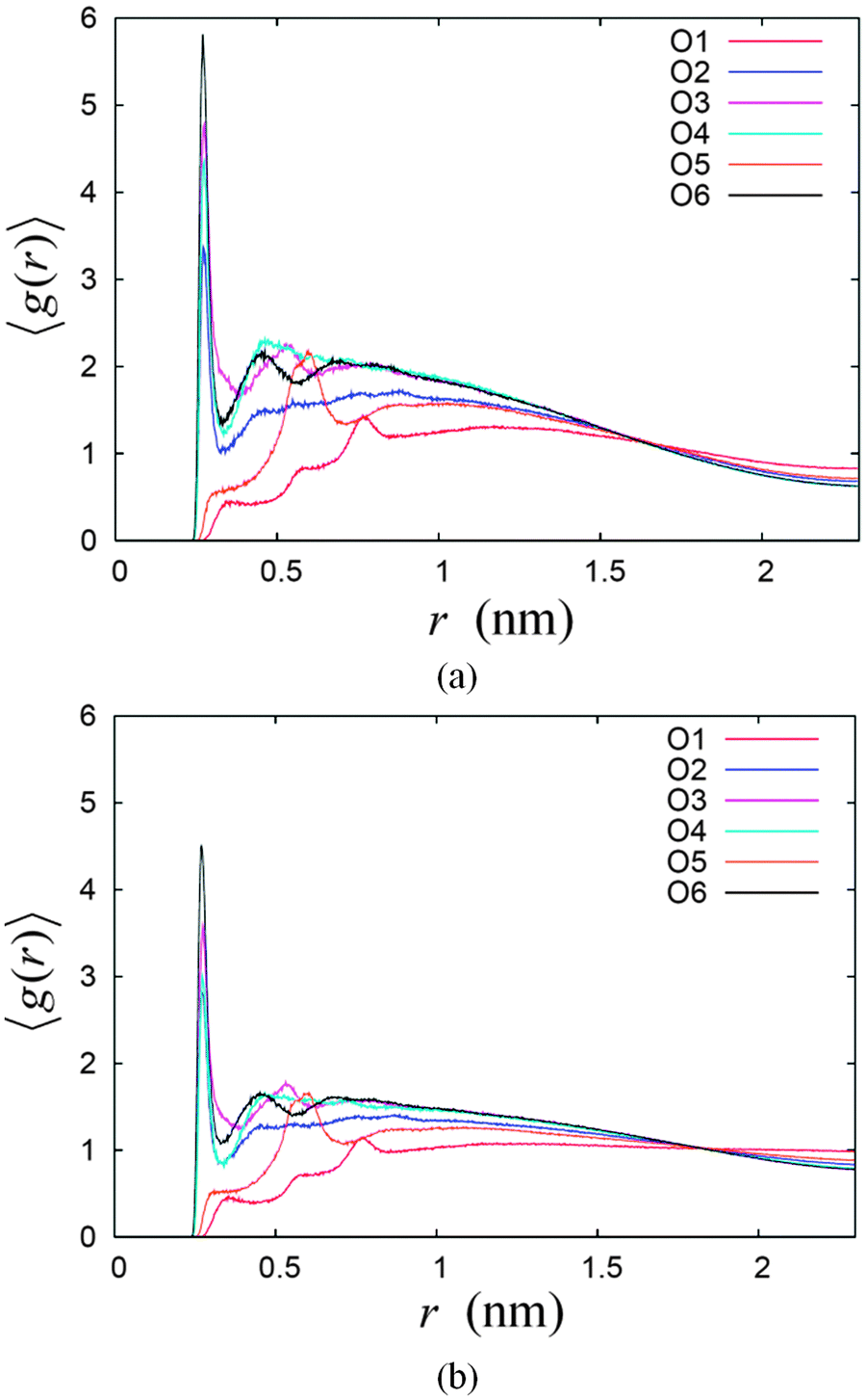 | ||
| Fig. 8 The radial distribution function (RDF) of water–oxygen around the six oxygen atoms for the two systems (a) 14% and (b) 22% water concentrations. | ||
| RDF | Peak positions (Å) | ||
|---|---|---|---|
| 1st | 2nd | 3rd | |
| RDF_O2 | 2.72 | Nil | Nil |
| RDF_O3 | 2.74 | 5.31 | Nil |
| RDF_O4 | 2.74 | 4.60 | Nil |
| RDF_O6 | 2.70 | 4.50 | 6.82 |
| RDF_OW67 | 2.88 | 4.50 | 6.73 |
On the other hand, RDF_O1 and RDF_O5 show the highest peak at the radial distance of 7.6 Å and 6.0 Å, respectively. The radial distances of these two peaks can be explained approximately as the distance of O1 and O5, to the water structure right outside the outermost region of water–sugar interface formed by O6–H, as explained previously. The estimated distances are obtained by approximating the distances of O1 and O5 to O6, i.e. 6.0 Å and 3.7 Å, plus the radial distance of first water structure for O6, which is 2.7 Å. This gives approximately 8.7 Å and 6.4 Å for O1 and O5, respectively which are close to their respective peaks positions in the RDF_O.
D. The packing of the alkyl chains
It is known that the cross-section of a column in the HII phase is not a smooth circular shape, but instead this is a hexagon with smooth corners.34,72–74 This hexagonal shaped column is necessary for the columnar structure to fill the space while maintaining the hexagonal lattice arrangement. This would mean the alkyl chains have to stretch out to the corner and be compressed on the face of the hexagon. The energy of compression and the extension of the alkyl chains is called the frustration energy.75 To see this effect in our simulation systems, we calculated the distribution of the radial distance for the methyl group, CH3 from the centre of its cylinder with respect to the angle around the column axis. We focused our analysis on the middle cylinder number 5 for the two systems from 10 ns to 50 ns, i.e. during the production stage.Fig. 9 gives the time averaged radial distances of CH3 from the centre of the cylinder as a function of the angle around the column for the two simulation systems. The averaged radial distances CH3 for the two systems peaked roughly at the six hexagonal corners, indicated by the vertical straight lines in Fig. 8. On the other hand, the radial distances of CH3 are lowest in between the two peaks, implying the compression of the alkyl chain at the faces of the hexagon. In Fig. 8, the non-uniform heights among the peaks and the dips indicate imperfection in the cylindrical symmetry of the columnar phase.
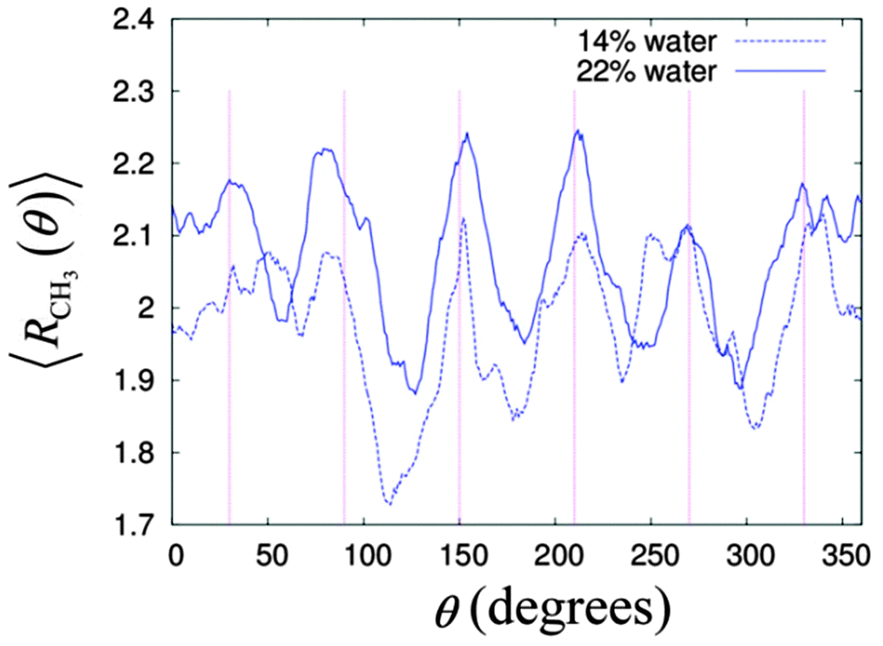 | ||
| Fig. 9 The distribution of the average radial distance of the CH3 over angles around the cylinder, where the straight vertical lines are at the angles 30°, 90°, 120°, 180°, 240° and 270°. | ||
IV. Conclusion
We have modelled and simulated the system of lyotropic HII formed by C8C12β-D-Glc at two different water concentrations, 14% and 22%, for simulation times of up to 50 ns. The average lattice parameters and area per head group obtained from the simulations for these two systems agree quantitatively to within the error with those estimated from the SAXS measurements. At the lower water concentration of 14% water the radial distribution of the density profile shows the sugar headgroup region and the water region overlap each other such that the water column is not completely free of the sugar headgroup. Meanwhile at the higher concentration of 22%, the region of water in the column does not overlap with the sugar headgroup. Two kinds of water diffusion process are observed. In the xy-plane the water mobility is anomalous for both the water concentration systems, in the z-direction for both systems however, the diffusion obeys Einstein's relationship. The anomalous diffusion in xy-plane is caused by confined space in the plane. The 10 ns time dynamics of water diffusion for the ‘free’ water and ‘bound’ in the 22% system were analysed. It was found the diffusion in the z-direction for the ‘free’ water is normal, while that of the ‘bound’ water is slightly anomalous. On the other hand, the diffusions in the xy-plane for both cases behave similarly to the overall water diffusion. Furthermore, at time less than 200 ps, the diffusion of ‘bound’ water is found to be slower compared that of the ‘free’ water. After 200 ps, the ‘bound’ water diffusion in the xy-plane became faster and saturated at higher averaged displacement values than that of the ‘free’ water, due to the exchange of water molecules from one region to another. Our findings provide an alternative explanation to the recent experimental results by Penaloza et al., who found the heterogeneity of diffusion in the water region of a lyotropic HII.63The interactions between the sugar head and water molecules were investigated by the hydrogen bond analysis and the calculations of RDF of water oxygen atoms around the six sugar oxygen atoms. In a system of 14% water the number of hydrogen bondings between water and sugar is lower but a longer lifetime was observed compared to the case of the 22% water system. This is attributed to the smaller surface area of water–sugar interface and lower mobility of water in the 14% water system compared to those of the 22% water system. The RDF of water oxygen atom around the six sugar oxygen atoms relates the level of contact or exposure of individual oxygen on sugar to the water molecules, which follows the ordering of O6 > O3 > O4 > O2 > O5 > O1 regardless of the water concentrations. Finally, we examined the extension and compression of the alkyl chain by calculating the distribution of average radial distance of the CH3 group over the angle around a cylinder. The profile of the distribution conforms to the picture depicted in the frustration theory.
Acknowledgements
We thank both the grants UM.C/625/1/HIR/MOHE/05 for supporting this project and RP001E-13ICT for supporting HSN. We also appreciate the computing resources provided by PTM University of Malaya.References
- R. Hashim, A. Sugimura, H. Minamikawa and T. Heidelberg, Liq. Cryst., 2012, 39, 1–17 CrossRef CAS.
- N. J. Brooks, H. A. A. Hamid, R. Hashim, T. Heidelberg, J. M. Seddon, C. E. Conn, S. M. Mirzadeh Husseini, N. I. Zahid and R. S. D. Hussen, Liq. Cryst., 2011, 38, 1725–1734 CrossRef CAS.
- V. Dembitsky, Lipids, 2004, 39, 933–953 CrossRef CAS PubMed.
- P. Jordan, P. Fromme, H. T. Witt, O. Klukas, W. Saenger and N. Krauss, Nature, 2001, 411, 909–917 CrossRef CAS PubMed.
- K. Gounaris and J. Barber, Trends Biochem. Sci., 1983, 8, 378–381 CrossRef CAS.
- V. Vill and R. Hashim, Curr. Opin. Colloid Interface Sci., 2002, 7, 395–409 CrossRef CAS.
- R. Hashim, H. H. A. Hashim, N. Z. M. Rodzi, R. S. D. Hussen and T. Heidelberg, Thin Solid Films, 2006, 509, 27–35 CrossRef CAS PubMed.
- R. N. A. H. Lewis, D. A. Mannock and R. N. McElhaney, in Current Topics in Membranes, ed. M. E. Richard, Academic Press, 1997, vol. 44, pp. 25–102 Search PubMed.
- D. A. Mannock, M. D. Collins, M. Kreichbaum, P. E. Harper, S. M. Gruner and R. N. McElhaney, Chem. Phys. Lipids, 2007, 148, 26–50 CrossRef CAS PubMed.
- M. Hato, H. Minamikawa, K. Tamada, T. Baba and Y. Tanabe, Adv. Colloid Interface Sci., 1999, 80, 233–270 CrossRef CAS.
- G. G. Shipley, J. P. Green and B. W. Nichols, Biochim. Biophys. Acta, Biomembr., 1973, 311, 531–544 CrossRef CAS.
- T. T. Chong, R. Hashim and R. A. Bryce, J. Phys. Chem. B, 2006, 110, 4978–4984 CrossRef CAS PubMed.
- V. Manickam Achari, H. S. Nguan, T. Heidelberg, R. A. Bryce and R. Hashim, J. Phys. Chem. B, 2012, 116, 11626–11634 CrossRef CAS PubMed.
- J. Kapla, B. Stevensson, M. Dahlberg and A. Maliniak, J. Phys. Chem. B, 2012, 116, 244–252 CrossRef CAS PubMed.
- V. Dembitsky, Lipids, 2005, 40, 869–900 CrossRef CAS PubMed.
- C. C. Ruiz, Sugar-based Surfactants: Fundamentals and Applications, Taylor & Francis, CRC Press, Boca Raton, 2009 Search PubMed.
- F. Nilsson, O. Söderman and I. Johansson, Langmuir, 1996, 12, 902–908 CrossRef CAS.
- A. J. O'Lenick Jr., J. Surfactants Deterg., 2001, 4, 311–315 CrossRef PubMed.
- M. Yasuda, Y. Arai, M. Kato, K. Uehara, O. Masakazu and T. Kurosawa, Jp. Pat. 09-020628, 1997 Search PubMed.
- T. Kaasgaard and C. J. Drummond, Phys. Chem. Chem. Phys., 2006, 8, 4957–4975 RSC.
- N. Ahmad, R. Ramsch, J. Esquena, C. Solans, H. A. Tajuddin and R. Hashim, Langmuir, 2011, 28, 2395–2403 CrossRef PubMed.
- I. Amar-Yuli, E. Wachtel, E. B. Shoshan, D. Danino, A. Aserin and N. Garti, Langmuir, 2007, 23, 3637–3645 CrossRef CAS PubMed.
- I. Amar-Yuli, E. Wachtel, D. E. Shalev, H. Moshe, A. Aserin and N. Garti, J. Phys. Chem. B, 2007, 111, 13544–13553 CrossRef CAS PubMed.
- I. Amar-Yuli, E. Wachtel, D. E. Shalev, A. Aserin and N. Garti, J. Phys. Chem. B, 2008, 112, 3971–3982 CrossRef CAS PubMed.
- I. Amar-Yuli, A. Aserin and N. Garti, J. Phys. Chem. B, 2008, 112, 10171–10180 CrossRef CAS PubMed.
- C. F. Black, R. J. Wilson, T. Nylander, M. K. Dymond and G. S. Attard, J. Am. Chem. Soc., 2010, 132, 9728–9732 CrossRef CAS PubMed.
- L. M. Crowe and J. H. Crowe, Arch. Biochem. Biophys., 1982, 217, 582–587 CrossRef CAS.
- B. de Kruijff, A. Rietveld and P. R. Cullis, Biochim. Biophys. Acta, Biomembr., 1980, 600, 343–357 CrossRef CAS.
- B. de Kruijff, A. M. H. P. van den Besselaar, P. R. Cullis, H. van den Bosch and L. L. M. van Deenen, Biochim. Biophys. Acta, Biomembr., 1978, 514, 1–8 CrossRef CAS.
- A. Stier, S. A. E. Finch and B. Bösterling, FEBS Lett., 1978, 91, 109–112 CrossRef CAS.
- I. Koltover, T. Salditt, J. O. Rädler and C. R. Safinya, Science, 1998, 281, 78–81 CrossRef CAS.
- S. Patil, D. Rhodes and D. Burgess, AAPS J., 2005, 7, E61–E77 CrossRef CAS PubMed.
- J. Corsi, R. W. Hawtin, O. Ces, G. S. Attard and S. Khalid, Langmuir, 2010, 26, 12119–12125 CrossRef CAS PubMed.
- J. M. Seddon, Biochim. Biophys. Acta, Rev. Biomembr., 1990, 1031, 1–69 CrossRef CAS.
- S. J. Marrink, A. H. de Vries and D. P. Tieleman, Biochim. Biophys. Acta, Biomembr., 2009, 1788, 149–168 CrossRef CAS PubMed.
- S. Bandyopadhyay, M. L. Klein, G. J. Martyna and M. Tarek, Mol. Phys., 1998, 95, 377–384 CrossRef CAS.
- I. D. Leigh, M. P. McDonald, R. M. Wood, G. J. T. Tiddy and M. A. Trevethan, J. Chem. Soc., Faraday Trans. 1, 1981, 77, 2867–2876 RSC.
- S. J. Marrink and D. Peter Tieleman, Biophys. J., 2002, 83, 2386–2392 CrossRef CAS.
- S. J. Marrink and A. E. Mark, Biophys. J., 2004, 87, 3894–3900 CrossRef CAS PubMed.
- V. Knecht, A. E. Mark and S. J. Marrink, J. Am. Chem. Soc., 2006, 128, 2030–2034 CrossRef CAS PubMed.
- V. Kolev, A. Ivanova, G. Madjarova, A. Aserin and N. Garti, J. Chem. Phys., 2012, 136, 074509–074511 CrossRef PubMed.
- H. A. A. Hamid, R. Hashim, J. M. Seddon and N. J. Brooks, Presented in part at the International Conference on Solid State Science & Technology, Melaka, December, 2012, Adv. Mater. Res. Search PubMed , in press.
- M. Hanwell, D. Curtis, D. Lonie, T. Vandermeersch, E. Zurek and G. Hutchison, J. Cheminf., 2012, 4, 17 CAS.
- T. A. Halgren, J. Comput. Chem., 1996, 17, 490–519 CrossRef CAS.
- C. Oostenbrink, A. Villa, A. E. Mark and W. F. van Gunsteren, J. Comput. Chem., 2004, 25, 1656–1676 CrossRef CAS PubMed.
- D. van der Spoel, E. Lindahl, B. Hess, G. Groenhof, A. E. Mark and H. J. C. Berendsen, J. Comput. Chem., 2005, 26, 1701–1718 CrossRef CAS PubMed.
- B. Hess, C. Kutzner, D. van der Spoel and E. Lindahl, J. Chem. Theory Comput., 2008, 4, 435–447 CrossRef CAS.
- H. J. C. Berendsen, J. P. M. Postma, W. F. Gunsteren and J. Hermans, in Intermolecular Forces, ed. B. Pullman, Reidel, Dordrecht, 1981, p. 331 Search PubMed.
- H. S. Nguan, T. Heidelberg, R. Hashim and G. J. T. Tiddy, Liq. Cryst., 2010, 37, 1205–1213 CrossRef CAS.
- D. Marsh, Chem. Phys. Lipids, 2011, 164, 177–183 CrossRef CAS PubMed.
- J. F. Nagle and S. Tristram-Nagle, Curr. Opin. Struct. Biol., 2000, 10, 474–480 CrossRef CAS.
- S. Granick, Science, 1991, 253, 1374–1379 CrossRef CAS PubMed.
- M. Heuberger, M. Zäch and N. D. Spencer, Science, 2001, 292, 905–908 CrossRef CAS PubMed.
- M. O. Jensen, O. G. Mouritsen and G. H. Peters, J. Chem. Phys., 2004, 120, 9729–9744 CrossRef CAS PubMed.
- N. Pérez-Hernández, T. Q. Luong, M. Febles, C. Marco, H.-H. Limbach, M. Havenith, C. Pérez, M. V. Roux, R. Pérez and J. D. Martín, J. Phys. Chem. C, 2012, 116, 9616–9630 Search PubMed.
- J. Tian and A. E. Garcia, J. Chem. Phys., 2011, 134, 225101–225111 CrossRef PubMed.
- J. Tian and A. E. Garcia, J. Am. Chem. Soc., 2011, 133, 15157–15164 CrossRef CAS PubMed.
- G. Hummer, J. C. Rasaiah and J. P. Noworyta, Nature, 2001, 414, 188–190 CrossRef CAS PubMed.
- F. Zhu and K. Schulten, Biophys. J., 2003, 85, 236–244 CrossRef CAS.
- G. M. Preston, T. P. Carroll, W. B. Guggino and P. Agre, Science, 1992, 256, 385–387 CAS.
- K. Murata, K. Mitsuoka, T. Hirai, T. Walz, P. Agre, J. B. Heymann, A. Engel and Y. Fujiyoshi, Nature, 2000, 407, 599–605 CrossRef CAS PubMed.
- E. Tajkhorshid, P. Nollert, M. Ø. Jensen, L. J. W. Miercke, J. O'Connell, R. M. Stroud and K. Schulten, Science, 2002, 296, 525–530 CrossRef CAS PubMed.
- D. P. Penaloza, K. Hori, A. Shundo and K. Tanaka, Phys. Chem. Chem. Phys., 2012, 14, 5247–5250 RSC.
- P. Mark and L. Nilsson, J. Phys. Chem. A, 2001, 105, 9954–9960 CrossRef CAS.
- A. Shundo, K. Mizuguchi, M. Miyamoto, M. Goto and K. Tanaka, Chem. Commun., 2011, 47, 8844–8846 RSC.
- Y. Bouligand, in Physical Properties of Liquid Crystals, ed. D. Demus, J. Goodby, G. W. Gray, H.-W. Spiess and V. Vill, Wiley-VCH, Weinheim, 1999, pp. 304–348 Search PubMed.
- A. K. Soper and M. G. Phillips, Chem. Phys., 1986, 107, 47–60 CrossRef CAS.
- A. Luzar and D. Chandler, Phys. Rev. Lett., 1996, 76, 928–931 CrossRef CAS.
- A. Luzar and D. Chandler, Nature, 1996, 379, 55–57 CrossRef CAS.
- D. van der Spoel, E. Lindahl, B. Hess, A. R. van Buuren, E. Apol, P. J. Meulenhoff, D. P. Tieleman, A. L. T. M. Sijbers, K. A. Feenstra, R. van Drunen and H. J. C. Berendsen, Gromacs User Manual version 4.5.4, www.gromacs.org, 2010 Search PubMed.
- D. van der Spoel, P. J. van Maaren, P. Larsson and N. Tîmneanu, J. Phys. Chem. B, 2006, 110, 4393–4398 CrossRef CAS PubMed.
- D. C. Turner and S. M. Gruner, Biochemistry, 1992, 31, 1340–1355 CrossRef CAS.
- S. Perutkova, M. Daniel, M. Rappolt, G. Pabst, G. Dolinar, V. Kralj-Iglic and A. Iglic, Phys. Chem. Chem. Phys., 2011, 13, 3100–3107 RSC.
- M. Hamm and M. M. Kozlov, Eur. Phys. J. B, 1998, 6, 519–528 CrossRef CAS.
- G. C. Shearman, B. J. Khoo, M. L. Motherwell, K. A. Brakke, O. Ces, C. E. Conn, J. M. Seddon and R. H. Templer, Langmuir, 2007, 23, 7276–7285 CrossRef CAS PubMed.
Footnote |
| † Electronic supplementary information (ESI) available. See DOI: 10.1039/c3cp52385c |
| This journal is © the Owner Societies 2014 |