Digital photography for the analysis of fluorescence responses†
Thimon
Schwaebel
,
Oliver
Trapp
and
Uwe H. F.
Bunz
*
Organisch-Chemisches Institut, Ruprecht-Karls-Universität Heidelberg, Im Neuenheimer Feld 270, 69120 Heidelberg, FRG. E-mail: Uwe.bunz@oci.uni-heidelberg.de
First published on 17th October 2012
Abstract
Different pyridine substituted cruciform fluorophores (XF) were prepared and their optical properties were studied. Upon protonation of the pyridine nitrogen, the XFs with a para or ortho substitution pattern show similar bathochromic shifts in the emission, whereas the meta XF features a smaller bathochromic shift in emission wavelength. The color changes of XFs in the presence of carboxylic acids were used to identify them by digital photography. Data extraction of the photographs is performed by a combination of a large RGB color space, a standard white balance, the transformation of RGB values into u′v′ values and MANOVA statistics, improving the recognition of analytes by pyridine XFs. We discuss in this paper factors that determine the quality of the extraction of color information from digital photograph.
Introduction
In this contribution we discuss issues relevant to the extraction of quantitative information from digital pictures of fluorescent dye-solutions in the presence of analytes (here carboxylic acids) that modulate fluorescence color and/or intensity.When successful, such concepts could potentially lead to simple “photographic” spectrometers then implemented in smart phone devices for the automatic interpretation of complex emissive/fluorescent test strips interacting with various analytes of clinical or environmental importance.
Fluorescent probes and sensors are critical in biological, analytical1 and environmental science.2 Consequently, application of fluorescent materials in biochemistry/cell biology led to the Nobel Prize for Tsien.3 Photography in combination with microscopy is established in cell biology for the effective staining of specific cell compartments. Analyte induced fluorescent changes are often documented by black and white photography using suitable filters.4 Fluorescence staining of electrophoretic gels is also recorded photographically.5 If fluorophores are applied in solution to test for an analyte or effector, fluorescence spectroscopy or fluorescence lifetime image microscopy (FLIM)6 are used most often. In combination with a plate reader and a 96-well plate, even relatively large data sets can be recorded spectroscopically.7 Such spectroscopic approaches are time consuming8 and need specialized, expensive equipment.
Fluorescence responses, recorded photographically, might be used in lieu of spectroscopic examination, as panels of photographs of fluorophore solutions exposed to different analytes (displaying significant color changes) are popular.9 Such an approach would be fast and inexpensive.
In the case of absorption, this panel-approach, combined with digital photography (via scanner) has successfully been exploited by Suslick et al.,10 Anslyn and Zhong11 or Mirkin et al.12 to analyze colorimetric responses of dyes towards series of different analyte classes. Photography of colorimetric changes is straightforward, lending itself to using greycards and color charts. Absolute and reproducible color descriptors result. In the case of fluorescence this is not possible, as one can only work with the emitted light.
Digital photography is successful in the analysis of fluorescent arrays, as we have identified amines13 and carboxylic acids14 using the change in the emission of specific cruciform fluorophores (XF)15 in different solvents. These XFs can have spatially separated frontier molecular orbitals, if the corresponding traverses are equipped with donor and acceptor substituents respectively. Such XFs display useful emission color changes when exposed to a multitude of different analytes, particularly metal salts (vide supra).
While discrimination of analytes by photography of fluorescence responses is possible for a given data set, different data sets of repeated experiments, prepared by different users, can vary significantly. Inherent difficulties in taking digital pictures of fluorescent samples include used excitation lamp and digital camera, sample positioning, exposure time and internal white balance. A combination of all these factors makes the quantitative reproducibility of fluorescence panels and their analysis challenging but also appealing and important due to simplicity and efficiency of photography as a tool.
A bit of color theory
A color model16a represents colors through a 3- or a 4-tupel, i.e. a vector containing 3 or 4 color components as in the RGB or the CMYK values. All of the possible combinations of these vectors (here either RGB or CMYK) then create a color space. Color spaces discern each other in that their gamut, i.e. the subset of colors that can be correctly described by the color space under consideration varies. The simple RGB color space for example cannot represent (see Fig. 1) certain green hues. | ||
| Fig. 1 Comparison of different color spaces in the u′v′ plane of color space CIE LUV; the black line displays all of the colors visible to the human eye. The attached numbers show the color of monochromatic light with the corresponding wavelength. The triangles represent three different RGB color spaces and E represents the white point. | ||
The most useful descriptor for color is a 2-dimensional (vide infra) projection of the CIE LUV values u′ and v′, see Fig. 1, that define the color but remove brightness information (vide infra).
In a simplified picture, humans and digital cameras alike report color using three different receptors, R (red), G (green), B (blue) from which they create “color”. However, eye and camera perceive different color spaces (Fig. 1); even the most advanced color space (ProPhoto RGB) available in digital image processing does not map the entire gamut of color perceived by the human eye. In the range of greenish and blue-to-purple hues even advanced color spaces are lacking. All of the missing but visible color points are then projected onto the edge of the respective triangle. Colors easily discerned by eye or spectral photometer are thus represented by identical (!) RGB values.
It would be attractive to convert RGB values from a photograph and spectral information from an emission spectrum into the same standardized color space (CIE LUV) to compare them. Evaluating the correct encoding of color information of digital photography by emission spectroscopy and storing emission data as numerical values in digital libraries, a digital photograph could be used for a quick identification of drugs, toxins or explosives, when employing a suitable sensory fluorophore.
Color information is transformed into numerical values according to the process depicted in Fig. 2. Central is the conversion of the emission spectrum or the RGB values into the tristimulus values (X, Y, Z) of the standardized color space CIE XYZ. These values are calculated from an emission spectrum using eqn (1)–(4):
 | (1) |
 | (2) |
 | (3) |
 | (4) |
 | ||
| Fig. 2 Depiction of color using spectral photometer or digital photography and their transformation into standardized CIE color spaces. | ||
P(λ) is the normalized emission spectrum and ![[x with combining macron]](https://www.rsc.org/images/entities/i_char_0078_0304.gif) , ȳ and
, ȳ and ![[z with combining macron]](https://www.rsc.org/images/entities/i_char_007a_0304.gif) are the CIE standard observer color matching functions (Fig. 3). X, Y and Z are mathematical constructs encoding visible colors with additive mixture of color stimuli. The value “Y” is unique, because it also represents brightness. The transformation of RGB into XYZ values depends on the RGB color space (see ESI†).
are the CIE standard observer color matching functions (Fig. 3). X, Y and Z are mathematical constructs encoding visible colors with additive mixture of color stimuli. The value “Y” is unique, because it also represents brightness. The transformation of RGB into XYZ values depends on the RGB color space (see ESI†).
 | ||
| Fig. 3 The CIE standard observer color matching functions of the color space CIE XYZ from 1931.16 | ||
The tristimulus values allow conversion of different color spaces into each other. CIE XYZ and the corresponding two-dimensional projection CIE xyY are useful and were already employed as tool in analytical chemistry.17 Comparing two colors, CIE xyY has the disadvantage that color differences are not equal, depending on the hue.18 The two dimensional projection u′ v′ of the equidistant color space CIE LUV is better. To convert XYZ into u′v′ values the eqn (5) and (6) are used:19
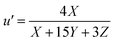 | (5) |
 | (6) |
In this u′v′ projection the color is shown only with its hue, the brightness coordinate Y is left out, but can be added if needed.
From a photograph one extracts RGB values, converts them into u′v′ coordinates via XYZ values. The typical digital camera does not fulfill the Luther conditions20 because the profiles of its filters do not look like the true color matching functions , ȳ and shown in Fig. 3. Photographing the fluorescence of several vials, each vial also has a slightly different position to the camera. The geometry i.e. distances and angels to the lens of the camera to measure color varies. Comparing calculated u′v′ values from photographs and emission spectra, differences in color coordinates are therefore expected. It is not clear if the two sets of data can be successfully mapped onto each other.
Results and discussion
Synthesis and spectroscopic properties of the XFs 5a–c
We have identified the pyridine-based XF 5a as an attractive reactive dye and have investigated the positional isomers of 5a, viz. 5b and 5c, in which the pyridine nitrogen are in the meta- and ortho-positions respectively to the styryl substituent. Starting from the bisphosphonate 1,21 Sonogashira coupling to the substituted phenylacetylene 2 furnished the bisphosphonate 3 in 80% yields after chromatography over silica gel. A double Horner reaction with suitable pyridine carboxaldehydes 4a–c afforded the XFs 5a–c22 in 60–74% yield after crystallization (Scheme 1). The single crystal X-ray structures of 5a–c show a planar conformation and display the expected bond lengths and bond angles. | ||
| Scheme 1 Synthesis of 5a–c. | ||
Fig. 4 displays the absorption and emission spectra of 5a–c in dichloromethane (top) and after addition of trifluoroacetic acid (bottom). The spectra of the unprotonated XFs 5a–c feature only subtle changes imparted by the position of the nitrogen in the ring. However, upon protonation, the spectra of 5a–c experience a bathochromic shift in both absorption and emission (Fig. 4, Table 1). The LUMO of 5a–c is localized on the styryl branches and protonating the pyridine nitrogen with trifluoroacetic acid stabilizes the LUMO more than the HOMO.15 The orbital coefficients of HOMO and LUMO of 5b are close to zero at the ring nitrogen atom as expected for a meta-positioned substituent (see ESI, Fig. S1†). Therefore red shift upon protonation is diminished in the emission spectrum of the meta-pyridine XF 5b.
 | ||
| Fig. 4 Normalized absorption and emission spectra of 5a–c (top) and in the presence (bottom) of trifluoroacetic acid (M) in dichloromethane. | ||
| Substance | λ absmax/nm | λ emmax/nm | υ st/cm−1 |
|---|---|---|---|
| XF 5a | 332 | 453 | 8045 |
| XF 5b | 332 | 451, 427 | 7948 |
| XF 5c | 334 | 456, 433 | 8010 |
| XF 5a + TFA | 340, 384sh, 446sh | 552 | 11![[thin space (1/6-em)]](https://www.rsc.org/images/entities/char_2009.gif) 296 296 |
| XF 5b + TFA | 334 | 487 | 94062 |
| XF 5c + TFA | 338, 390sh, 454sh | 543 | 11170 |
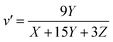
Sensor panels using 5a–c and a selection of acids
After the optical properties of 5a–c were investigated, we tested their differentiating ability with a selection of organic acids in different solvents (Scheme 2, Fig. 5). The pKa values14,23 of the tested carboxylic acids B–M are reported and defined for water and may differ in other (organic) solvents. This should not be an issue, as the identification of the acids does not only depend on their pKa but also on other factors that influence their ability to form complexes with the pyridine nitrogen and the overall π-system of the XF. The fundamental working principle of this detection system rests upon coordination of a positive charge (proton here) to the pyridine unit of the XF, leading to a stabilization of the LUMO, leaving the HOMO unchanged and resulting in a predominant stabilization of the excited state. Red shifted emission features result.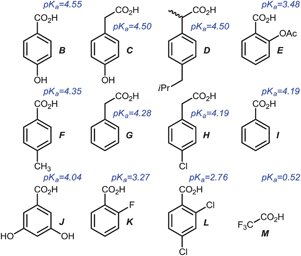 | ||
| Scheme 2 Structurally related carboxylic acids and their pKa value14,23 in water used as model analytes. | ||
 | ||
| Fig. 5 Photography of 5b (top), 5c (middle) and 5a (bottom) (file format: JPEG, color space: sRGB) in the presence of different carboxylic acids (B–M; A = reference) in different solvents recorded at a shutter speed of 0.1 s. (calibration data set). | ||
The setup for recording the fluorescence of the solution was adapted from our previously established protocols (see ESI, Fig. S3†).14 The twelve samples were placed in 5 mL drum vials on a handheld UV-light source (excitation wavelength 365 nm). The concentration of the XF was 1 μM and that of the carboxylic acids 0.13 M. The photographs were taken with a Canon EOS7D camera (objective: EF-S60mm F/2.8 Macro USM) at a distance of 75 cm. Focal aperture (F2.8) and film sensitivity (ISO 100) were kept constant. The shutter speed changed from 0. 2 s to 0.04 s.
The para-substituted XF 5a (Fig. 5, bottom) displays the largest color shifts when exposed to different carboxylic acids. The meta-pyridine based 5b displays the smallest shifts in emission color, as expected from the lack of a coefficient in the LUMO (see ESI, Fig. S1†) on the pyridine nitrogen. The pyridine XF 5c is only slightly better in performance than 5b. Only for strong acids, such as TFA, the color response of 5c is similar to that of 5a. The differences between 5a and 5c are not so much electronic in nature but due to induced twisting probably necessary for the weaker acids to bind to the pyridine nitrogen. Therefore XF 5a is best suited to recognize carboxylic acids.14
The addition of acid J to any of the XF solutions (Fig. 5) appears to shift the emission color to the blue. The shift is deceptive as only quenching is observed; according to fluorescence spectroscopy there is no blue-shift (see ESI, Fig. S14†).
Strategy and implementation of photographic workup
The fluorescence of a solution can be recorded with any digital camera in the file format JPEG. Digital reflex cameras record a picture in either two file formats, JPEG or RAW. The RAW format needs additional picture processing (i.e. in Adobe® Photoshop® CS5), in which color space and white balance are set. The RGB (range from 0 to 255) extraction encompasses a spot of 141 × 141 pixels with statistical information (see ESI, Fig. S4†).RGB values of fluorescent solutions obtained from photographs are dependent upon brightness. Fig. 6 displays a panel of XF 5c, 5c + 4-methylbenzoic acid (F), 5c + 2-fluorobenzoic acid (K) and 5c + trifluoroacetic acid (M) at eight different shutter speeds (0.2 s to 0.04 s) using JPEG (with automatic changing white point) and RAW data formats. To extract the hue, the RGB values were transformed into the u′v′ Y color space (Y: brightness). All of the photographs taken with different shutter speeds should display the same u′ and v′ values for the color. However, this is not the case for the JPEG format when there is no set white balance. In the u′v′ Y color space (related yet only different from the CIE LUV color space, where the white point is set to be the origin) the four hues show significant changes (Fig. 6 red arrows) in dependence of the shutter speed.
 | ||
| Fig. 6 (A, bottom) photography (format: JPEG; color space: sRGB; white balance: automatic) of 5c in the presence of three different organic acids (A = reference; F = 4-methylbenzoic acid, K = 2-fluorbenzoic acid, M = trifluoroacetic acid) in dichloromethane recorded with different shutter speeds (0.2–0.04 s); (A, top) projection of the extracted and transformed RGB values onto the u′v′ plane of the u′v′Y color space. (B) Same recorded pictures as in (A) but processed differently (format: RAW; color space: ProPhoto RGB; white balance: constant). | ||
If the same recorded pictures (format RAW) are processed with a set white balance and color space (settings in Adobe® Photoshop® CS5: color temperature: 6500 K; hue = 0; color space: ProPhoto RGB) the situation improves considerably (Fig. 6B). For the rows A to M, the match is more satisfying (red circles) but the u′v′ values still depend on the shutter speed. The first two to three values for A and K show a significant deviation, resulting from an incorrect description of color with RGB values as one value of RGB suffers from an “overflow”. Reducing the shutter speed, all values of RGB decline and below a threshold point value and the hues are described correctly. To conclude: a fixed white balance combined with a slight underexposure when taking pictures from fluorescent solutions is strongly recommended.
Color recognition using digital photography
From the preliminary studies (Fig. 5) we selected XF 5a to perform further color recognition tests with data obtained at two different shutter speeds 0.1 s, 0.04 s), processed into different data formats (RAW, JPEG) and color spaces (sRGB, Adobe RGB, ProPhoto RGB). The RGB values of each color space and the transformed u′v′ values were then processed by multivariate analysis of variance (MANOVA).24In this analysis we compare numerical values from digital pictures of a test data set with those of a calibration set containing n (test) or m (calibration) analyte–fluorophore–solvent combinations (patch) per photograph. Here each analyte fluorophore complex (AFC) is investigated in six different solvents resulting in six patches with a total number of 18 RGB values or better 12 u′v′-values.
To obtain a correlation plot, a differential sigma value σn,m has to be obtained for every combination of AFC(test) with AFC(calibration). σn,m is calculated with eqn (7) or (8):
 | (7) |
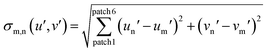 | (8) |
The number of patches per analyte is herein defined by the number of fluorophores multiplied by the number of solvents used. The primary expression under the root sign is the statistical difference between two to each other corresponding patches. If the two directly compared patches are increasingly different in color, increasingly large σ-values for this pair result. The algebraic sign of the difference (for example un′ − um′) is immaterial, as it is squared and therefore always positive. Summation over these six values gives σn,m, the direct measure of the discernibility of two samples. X (12 here) different analytes (carboxylic acids) therefore give a matrix of x2, (here 144) σn,m values.
If σn,m values are obtained for one data set (i.e. the data are auto-cross correlated, in a control set) a symmetrical matrix results in which the diagonals all must be equal zero. This control matrix gives a way to test the intrinsic quality of the chosen experiment under optimum conditions. If the analyte–fluorophore–solvent combinations allow perfect differentiation, then all non-diagonal fields of the matrix should show large values. In a completely failed experiment, all elements of the matrix would be zero, i.e. all values of σn,m would be zero and none of the investigated analytes could be discerned. An example for a σn,m matrix obtained by us is shown in Fig. 7. The size of the matrix is defined by the number of analytes plus the photograph of the blank fluorophore solution. This approach is somewhat crude but quite effective in interpreting analyte-induced color changes in fluorophore solutions.
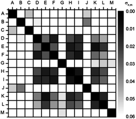 | ||
| Fig. 7 Autocorrelation plot (u′v′ values) of fluorescent solutions of 5a in the presence of carboxylic acids recorded with a digital camera (RAW; color space: ProPhoto RGB; white balance: 6500 K) taken with shutter speed 0.1 s (C 0.1 s). When color information of identical carboxylic acids + 5a is correlated, the deviation σn,m disappears (black squares on the diagonal). | ||
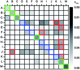
The used example for the correlation plot of the calibration data sets with the color space ProPhoto RGB, transformed into u′v′ values for shutter speeds 0.1 s (C 0.1 s; C = calibration) and 0.04 s (C 0.04 s), show similar patterns. Both autocorrelation sets discern the acids from each other using photography (Fig. 8 and S30†). However, some combinations with acids such as ibuprofen (D), aspirin (E), para toluic acid (F), 4-chlorophenylacetic acid (H) and benzoic acid (I) or 2-fluorobenzoic acid (K) and 2,4-dichlorobenzoic acid (L) are almost indistinguishable using only 5a in six solvents. The data set with a smaller shutter speed gives better results, not surprising in the light of the discussed issues. The next step was to record digital pictures (test data set) of XF 5a with the acids (B–L) in an unknown order (2–12, Fig. 8) with shutter speeds of 0.1 s (T 0.1 s; T = test) and 0.04 s (T 0.04 s). The reference A, XF 5a, was kept constant on the position 1. The calibration set with the shutter speed 0.1 s (C 0.1 s) matches best up with T 0.04 s. Photographs of these two sets qualitatively looked “most similar” by eye. Fig. 9 represents the correlation C 0.1 s versus T 0.04 s (Table 2, entry 8). Ten out of twelve patches were recognized. Benzoic acid (I, row 4) was mismatched to 4-methylbenzoic acid (F) which in turn (row 9) was mismatched to ibuprofen (D). This result is quite impressive as we have used only one dye (5a) in six different solvents.
 | ||
| Fig. 8 Example of the photographs of the test sets (unknown order for the acids except for 1; 1 = XF 5a), in which the samples were recorded with shutter speeds of 0.1 s (top, T 0.1 s) and 0.04 s (bottom, T 0.04 s). The numbers encode the position of the sample on the picture (order of the test data set: 1 = A, 2 = E, 3 = K, 4 = I, 5 = C, 6 = L, 7 = H, 8 = G, 9 = F, 10 = D, 11 = J, 12 = B). | ||
 | ||
| Fig. 9 Correlation plot of T 0.04 s with C 0.1 s using u′v′ values (converted from RAW, ProPhoto RGB picture). The test data set is encoded with numbers. Black squares implement a small and white squares a high color difference as expressed in σ values (order of the test data set: 1 = A, 2 = E, 3 = K, 4 = I, 5 = C, 6 = L, 7 = H, 8 = G, 9 = F, 10 = D, 11 = J, 12 = B). The green squares mark the correctly identified acids; the red squares mark the misidentified and the blue squares mark the corresponding correct acids. | ||
| Entry | Color space | C 0.1 s | C 0.04 s | ||
|---|---|---|---|---|---|
| T 0.1 s | T 0.04 s | T 0.1 s | T 0.04 s | ||
| 1 | RGB | 4/12 | 8/12 | 2/12 | 2/12 |
| 2 | u′v′ | 5/12 | 7/12 | 2/12 | 4/12 |
| 3 | RGB | 4/12 | 9/12 | 3/12 | 3/12 |
| 4 | u′v′ | 7/12 | 10/12 | 7/12 | 8/12 |
| 5 | RGB | 3/12 | 8/12 | 2/12 | 3/12 |
| 6 | u′v′ | 6/12 | 11/12 | 6/12 | 9/12 |
| 7 | RGB | 2/12 | 7/12 | 2/12 | 3/12 |
| 8 | u′v′ | 7/12 | 10/12 | 6/12 | 10/12 |
The data in Table 2 concentrates the promising results. Using RGB (not u′v′) values, the MANOVA analysis works best if the pictures of the data sets look similar (C 0.1 s and T 0.04 s). Up to 9/12 samples (entry 3) are correctly recognized. Overexposed or highly exposed photographs lose color information (Fig. 6B).
For photographs recorded in format JPEG (white point: automatic; color space: sRGB), RGB values do not fare well and transformation into the u′v′-space did not help either (Table 2; C 0.1 s T 0.04 s, entries 1 and 2) except for similar looking pictures. In the case of format RAW (white point: constant; color space: sRGB, Adobe RGB or ProPhoto RGB) the RGB values also do a decent job, when similar photographs are used (Table 2; C 0.1 s, T 0.04 s, entries 3, 5 and 7). If the RGB values are transformed into the u′v′ color space, recognition improves, in some cases dramatically (from 3/12 to 10/12; Table 2; C 0.04 s T 0.04 s, entry 7 and 8). The use of u′v′ with the correct data format (RAW; constant white balance) and the expanded color space (ProPhoto RGB) allows then, if the photographs are not overexposed, the most successful recognition of the analyte acids (Table 2; C 0.1 s, T 0.04 s, entry 8; C 0.04 s, T 0.1 s, entry 8). This composite choice allows the best description of color.
Color recognition using converted emission spectra
Emission spectra are converted into u′v′ values using eqn (1)–(6). The autocorrelation plot from the spectral information performed on A–M (Fig. 10, left) shows similarities to the autocorrelation plot of the photographs (Fig. 7). The AFCs of acids K and L or I and D, E, F, H are hard to differentiate from each other, not surprising, as photography and emission spectroscopy contain fundamentally the same optical information (Fig. 2). | ||
| Fig. 10 Left: autocorrelation plot of emission spectra converted into u′v′ numerical values. Right: correlation plot of a test data set with the calibration set using u′v′ values converted from emission spectra. The test data set is encoded with numbers. Black squares implement a small and white squares a high deviation (σn,m) from test data set to calibration data set (order of the test data set: 1 = A, 2 = H, 3 = C, 4 = F, 5 = K, 6 = I, 7 = J, 8 = D, 9 = G, 10 = L, 11 = E, 12 = B). The green squares mark the correctly identified acids; the red squares mark the misidentified and the blue squares mark the correct acids. | ||
Using the u′v′ values of the emission spectra, MANOVA statistics identified eleven out of twelve samples from a test data set, spectroscopy being only marginally better than our photographic results. Only benzoic acid (row 6) could not be identified correctly, because the smallest deviation belonged to both aspirin (E) and benzoic acid (I) of the calibration set (Fig. 10, right, row 6). Using a spectral photometer, converting spectral information into u′v′ value and MANOVA statistical analysis, identification of unknown carboxylic acids works well, but surprisingly not much better than by data extraction from photographs.
Having an additional data set of u′v′ coordinates makes it possible to analyze the u′v′ data set of the photographs employing the data set extracted from the emission spectra. The autocorrelation graphs show a similar pattern for the data sets taken with the spectral photometer or with the camera (Fig. 7, Fig. S6,† and Fig. 10 left). We compared the u′v′ values (emission spectra) with u′v′ values of the photographs as test sets (Fig. 11, Fig. S31†). The analysis included C 0.1 s and C 0.04 s data set obtained from digital pictures processed in the color space ProPhoto RGB. The order of the data sets was known. Ideally, the correlation plot should show black squares on the diagonal. Six out of thirteen AFCs could be identified independently from the shutter speed. For both data sets the patches A, B, C, G, L and M, which show the greatest color changes, were identified correctly.
 | ||
| Fig. 11 Correlation plots of u′v′ values with the calibration data set of the emission spectra and the calibration data set of the pictures (C 0.1 s). The green squares mark the correctly identified acids; the red squares mark misidentified and the blue squares mark the correct acids. | ||
A closer look at the coordinates of the u′v′ values show systematic drifts for all colors observed for any solvents and shutter speeds (Fig. 12). The camera uses internal algorithms to convert the color for the file format JPEG; for the RAW format Adobe Photoshop (Camera RAW converter) processes the data. However, the systematic drifts seem to be depending on the u′v′ value of the photograph. Therefore, it should be possible to construct a vector field in which any u′v′ point obtained by a camera is corrected and assigned to correct “spectroscopic” u′v′ values.
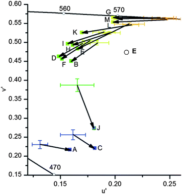 | ||
| Fig. 12 Comparison of the u′v′ values recorded with a digital camera (cross; C 0.1 s; color space ProPhoto RGB; error bars are calculated from the standard deviation) and converted from emission spectra (squares; wavelengths ± 1 nm, therefore error bars are negligible) from samples dissolved in acetonitrile. Data of identical substances are connected with an arrow. The black line represents the border of the color space of the human eye and E with the circle represents the white point. | ||
Questions that still remain are (a) if the vector field can be analytically expressed and therefore be used to transform photographic into “spectroscopic” data and (b) how different are the vector fields for different types of cameras? An answer would be attractive, as for example the cameras included in cell phones might be used as primitive RGB or u′v′ “spectrometers”. One more issue is however, that, while a specific emission spectrum unequivocally gives one RGB or u′v′ value, a specific RGB or u′v′ value can be constructed by – in principle – an infinite number of different emission spectra. As an example, white light can either be obtained from a black-body radiator like a light bulb or by mixing red, green and blue emission like in an LED. This problem however, is less of an issue if fluorophores with only one emission feature are employed.
Photography and fluorescence spectrometer work well to identify the acids, but surprisingly, the spectroscopic method does not work much better. Both methods record the same information and transform it into the selected color space. But interpreting spectral data by photography and vice versa is still difficult. This process should be more facile if a suitable vector field is used to correct the photographic u′v′ values and to transform them into “spectral” data.
Digital cameras are cheap, ubiquitous and unspecialized and allow acquiring large amounts of information quickly. Here we have obtained the information content of 12 emission spectra in less than a second. This powerful approach offers itself up for quality control challenges where fluorescent dyes and their color changes are critical, but also where it is desired to extract spectral information from photographs.
Conclusions
We have delineated factors that define the photographic analysis of color changes in fluorophore solutions in the presence of analytes. We have developed a fairly simple process in which optimized photographical data acquisition, processing and statistical workup are outlined tutorial-style. Data processing and treatment is critical in this approach. Also, we have compared RGB or u′v′-values obtained from photography with those from emission spectra. While a digital camera cannot yet be directly used as a quick RGB or u′v′ spectrometer, it should be possible to develop a vector field that would enforce this conversion. Therefore it should be possible to directly compare and use libraries of RGB or u′v′ values obtained from fluorescent solutions. The use of u′v′ value gives only the hue of a color, but not its brightness. We want to develop this method into a photographic emission “spectrometer”. Uses of such would include but not be restricted to analyzing complex fluorescent test strips by a small gadget that uses a cellphone as both spectrometer but also with a suitable app as a way to analyze complex data sets. Quality control would be an attractive future application of this concept.Acknowledgements
We thank the Struktur und Innovationsfond des Landes Baden-Württemberg for the funding of the necessary equipment (fluorimeter, UV-vis spectrometer and camera).Notes and references
-
(a) L. A. Cabell, M. D. Best, J. J. Lavigne, S. E. Schneider, D. M. Perreault, M. K. Monahan and E. V. Anslyn, J. Chem. Soc., Perkin Trans. 2, 2001, 315–323 RSC
; (b) S. W. Thomas, G. D. Joly and T. M. Swager, Chem. Rev., 2007, 107, 1339–1386 CrossRef CAS
-
(a) L. C. Yang, R. McRae, M. M. Henary, R. Patel, B. Lai, S. Vogt and C. J. Fahrni, Proc. Natl. Acad. Sci. U. S. A., 2005, 102, 11179–11184 CrossRef CAS
- B. N. G. Giepmans, S. R. Adams, M. H. Ellisman and R. Y. Tsien, Science, 2006, 312, 217–224 CrossRef CAS
- E. Moczko, I. V. Meglinski, C. Bessant and S. A. Piletsky, Anal. Chem., 2009, 81, 2311–2316 CrossRef CAS
- See for example: Q. Huang and W. L. Fu, Clin. Chem. Lab. Med., 2005, 43, 841–842 CrossRef CAS
- P. I. H. Bastiaens and A. Squire, Trends Cell Biol., 1999, 9, 48–52 CrossRef CAS
- U. H. F. Bunz and V. M. Rotello, Angew. Chem., Int. Ed., 2010, 49, 3268–3279 CrossRef CAS
-
(a) M. De, S. Rana, H. Akpinar, O. R. Miranda, R. R. Arvizo, U. H. F. Bunz and V. M. Rotello, Nat. Chem., 2009, 1, 461–465 CrossRef CAS
-
(a) J. Lim, T. A. Albright, B. R. Martin and O. S. Miljanic, J. Org. Chem., 2011, 76, 10207–10219 CrossRef CAS
-
(a) N. A. Rakow and K. S. Suslick, Nature, 2000, 406, 710–713 CrossRef CAS
- Z. L. Zhong and E. V. Anslyn, J. Am. Chem. Soc., 2002, 124, 9014–9015 CrossRef CAS
-
(a) R. Elghanian, J. J. Storhoff, R. C. Mucic, R. L. Letsinger and C. A. Mirkin, Science, 1997, 277, 1078–1081 CrossRef CAS
-
(a) P. L. McGrier, K. M. Solntsev, S. Miao, L. M. Tolbert, O. R. Miranda, V. M. Rotello and U. H. F. Bunz, Chem.–Eur. J., 2008, 14, 4503–4510 CrossRef CAS
- E. A. Davey, A. Zucchero, O. Trapp and U. H. F. Bunz, J. Am. Chem. Soc., 2011, 133, 7716–7718 CrossRef CAS
-
(a) A. J. Zucchero, P. L. McGrier and U. H. F. Bunz, Acc. Chem. Res., 2010, 43, 397–408 CrossRef CAS
- (a) We found the best accessible reference for the definition of color space http://en.wikipedia.org/wiki/Absolute_color_space in Wikipedia; (b) Color and Vision Research Laboratory http://cvrl.ioo.ucl.ac.uk/.
- R. C. Evans and P. Douglas, Anal. Chem., 2006, 78, 5645–5652 CrossRef CAS
- D. L. MacAdam, J. Opt. Soc. Am., 1942, 32, 247–273 CrossRef
- DIN 5033, Color Measurement. See Wikipedia CIE 1931 color space.
- R. Z. Luther, Sov. Phys. Tech. Phys., 1927, 8, 540–558 Search PubMed
- J. N. Wilson, P. M. Windscheif, U. Evans, M. L. Myrick and U. H. F. Bunz, Macromolecules, 2002, 35, 8681–8683 CrossRef CAS
- A. J. Zucchero, J. N. Wilson and U. H. F. Bunz, J. Am. Chem. Soc., 2006, 128, 11872–11881 CrossRef CAS
-
W. M. Haynes, CRC Handbook of Chemistry and Physics, Mohr & Tailor, 84th edn, 2004 Search PubMed
- S. Sekulic, M. B. Seasholtz, Z. Y. Wang, B. R. Kowalski, S. E. Lee and B. R. Holt, Anal. Chem., 1993, 65, 835–845 Search PubMed
Footnote |
| † Electronic supplementary information (ESI) available: Synthesis of the compounds 3, 5a–c, quantum chemical calculation of the frontier orbitals of 5′a–c, [5′a + 2H]2+, [5′b + 2H]2+ and [5′c + 2H]2+; extraction and transformation of RGB values into u′v′ values for different RGB color spaces; transformation of emission spectra into u′v′ values, MANOVA statistics for all autocorrelation and correlation plots. See DOI: 10.1039/c2sc21412a |
| This journal is © The Royal Society of Chemistry 2013 |