The influence of charge ratio on transient networks of polyelectrolyte complex micelles

Abstract

We study the influence of charge ratio on the transient network formation of bridged polyelectrolyte complex micelles. The polyelectrolyte complex micelles are based on mixing an ABA triblock copolymer in which the A-blocks are positively charged and the B-block is neutral and hydrophilic, and a negatively charged homopolymer. We investigate the microstructure of our samples with (dynamic) light scattering and small-angle X-ray scattering, and the mechanical properties by rheometry. At charge stoichiometric conditions, we obtain flowerlike polyelectrolyte complex micelles. These micelles become interconnected at high concentrations, leading to a sample-spanning transient network. For excess negative charge conditions, we obtain so-called ‘soluble complexes’ which are small aggregates carrying the excess negative charge on the polyelectrolyte complex parts. For excess positive charge conditions, micelles stay intact, because the triblock copolymers can localize the excess positive charge at the periphery of the micellar corona. This structural asymmetry is not reflected in the mechanical properties, which show a strong decrease in viscosity on either side of the charge stoichiometric point.

---

Introduction

The mechanical properties of liquids can be drastically altered by incorporation of a network forming agent. In physical gels the network consists of non-permanent cross-links that can break and reform continuously, contrary to covalently cross-linked chemical gels. This makes physical gels responsive to external stimuli. It also enables the relaxation of internal stresses, meaning that physical gels are essentially liquid-like.

For environmental reasons, water is the ideal solvent for applications. There are many examples of water-based physical gels, of which the hydrophobically end-capped polyurethane associative thickeners are most extensively studied and applied.^1–6 In these systems hydrophobic groups on the extremities of a long polymeric spacer cluster together to form micellar nodes. Hydrophobicity of the end-blocks is the driving force in many other examples of water-based transient networks.^7–10 Some of the possibilities for reversible network formation have recently been reviewed.¹¹

Of all driving forces for association, electrostatic interaction is possibly the most versatile. There are, however, only a few examples of transient networks in which electrostatic interactions play a key role.^12,13 Recently, we developed a water-based two component physical gel based on electrostatic interactions only. We have achieved this by mixing an aqueous ABA triblock copolymer solution, in which the A blocks are negatively charged and the B block is neutral and hydrophilic, with an aqueous solution of positively charged homopolymer. The two polymeric components interact to form a well defined multi-responsive transient network of interconnected polyelectrolyte complex micelles.¹⁴

Dilute solutions of polyelectrolyte complex micelles have been studied for quite some years,^15–17 and this has led to a basic understanding of the principles governing the properties of polyelectrolyte complex micelles in dilute solutions.^18–20 Understanding the dominant phenomena in charge-driven association was key to the creation of more ‘exotic’ types of polyelectrolyte complex micelles.^21–23

A defining property of polyelectrolyte complex micelles is that at least two oppositely charged moieties are needed to create a driving force for association. This implies that charge composition is a new variable: one can mix, or synthesize, the charged moieties in different ratios. Since electrostatic interaction is the driving force for association, it is most convenient to express the composition of the charged moieties in terms of charge ratio. The influence of charge ratio on micellar systems has been recognized from the beginning,¹⁵ and it is now well established that the association of the oppositely charged moieties is strongest at a 1 : 1 charge ratio.^17,24–29 This is not only valid for polyelectrolyte complex micelles, but is a generic feature of charge-driven association.^20,30–33 On the contrary, it is much less clear what happens to the polyelectrolyte complex micelles away from the charge stoichiometric point. Generally it is assumed that excess charge accumulates in the polyelectrolyte complex, which progressively destabilizes the micelles, making them eventually fall apart into so-called ‘soluble complexes’,^17,24 a term originally assigned to non-stoichiometric complexes of two oppositely charged homopolymers.³⁴

The dependence of the transient network topology on concentration and ionic strength at charge stoichiometric conditions has been described recently.³⁵ However, what happens to transient networks of interconnected polyelectrolyte complex micelles away from the charge stoichiometric point has never been investigated, despite charge composition being a crucial parameter in charge-driven association. Understanding the role of charge composition is also of industrial interest, for it is another parameter to tune the mechanical properties of this water-based multi-responsive two-component rheology modifier.

Here we present a study on the influence of charge ratio on transient networks of polyelectrolyte complex micelles. We do so by preparing polyelectrolyte complex micelles and their transient networks in an analogous manner as in previous studies,^14,35 with the difference that in this paper we use a triblock copolymer with positively charged end-blocks and a negatively charged homopolymer. We vary the charge composition, while keeping the total polymer concentration constant. Scattering techniques in combination with rheometry clarify the microstructure at non-stoichiometric conditions. We find a remarkable asymmetry in the microstructure at the two different sides of the stoichiometric composition, which is not reflected in the mechanical behaviour of our gels.

Experimental

Triblock copolymer synthesis

The triblock copolymer was synthesized in two steps. First, a bifunctional macro-initiator was synthesized based on the method by Jankova and coworkers.³⁶ The detailed synthetic protocol has been described elsewhere.¹⁴ In brief, poly(ethylene glycol) of M_n = 10 kg mol⁻¹ (Fluka, PDI = 1.04) was dissolved in toluene. After addition of triethylamine and 2-bromoisobutyryl bromide, the reaction mixture was stirred for five days at 30 °C. Purification was performed by treatment with charcoal, filtration, precipitation in petroleum ether, filtration, redissolving in THF and precipitation in petroleum ether (twice), filtration and drying overnight under vacuum. The degree of esterification was 100% as determined by ¹H-NMR.^37,38

The bifunctional macro-initiator was used to synthesize the triblock copolymer by atom transfer radical polymerization,^39,40 based on the method described by Li and coworkers.⁴¹ In detail, 11.8 g of the bifunctional macro-initiator was mixed with 21.2 g [2-(methacryloyoxy)ethyl] trimethylammonium chloride (Sigma Aldrich, 78wt% in water), 0.9 g bipyridyl (Acros Organics, 99+ %), 2-propanol and deionized water. The solvent ratio was 1 : 1 (v/v). The mixture was stirred and placed in an oil bath at 40 °C, while removing oxygen by bubbling argon for 45 min. Subsequently, 1.1 mmol Cu(I)Cl and 1.1 mmol Cu(II)Cl₂ were added to the mixture to start the reaction. After two hours, additional degassed solvent was added to facilitate stirring. After a total of five hours, the reaction was quenched by bubbling oxygen through the mixture. The product was purified by dialysis against DI-water for three days, refreshing the dialysis bath every day. After the partial removal of water by evaporation under reduced pressure, the product was obtained by freeze-drying overnight. The yield by weight was 73% (20 g). On average 68 monomers were attached per macro-initiator molecule, as determined by ¹H-NMR, see supporting information.

Homopolymer synthesis

Preparation of the negatively charged homopolymer was based on the work of Masci and coworkers.⁴² 15.2 g of 3-sulfopropylmethacrylate potassium salt (KSPMA) (62 mmol) was dissolved in approximately 25 ml DI-water/DMF (volume 1 : 1). The mixture was continuously stirred at approximately 45 °C while removing oxygen by bubbling argon for approximately one hour. Then 167 mg bipyridyl, 28.5 mg Cu(II)Cl₂ followed by 20.8 mg Cu(I)Cl were added to the mixture. To start the polymerization, 45.3 mg (0.23 mmol) of 2-EBiB was added, aiming for a degree of polymerization of approximately 260. The reaction mixture was left for 22 h to react.

The reaction was quenched by bubbling oxygen through the reaction mixture, and addition of DI-water. The product was purified by dialysis against 1.0 M KCl (3×), to remove the copper catalyst, and DI-water (3×). After filtration of the solution over a 0.2 μm syringe filter and removal of excess water by evaporation at reduced pressure, the product was obtained by freeze-drying overnight. The yield was determined to be 71% by weight (10.8 g).

¹H-NMR could not be used to determine the degree of polymerization, since the signal from the protons in the initiator is too weak to be accurately compared with the signal from the SPMA monomers. Size exclusion chromatography indicated an average degree of polymerization of 173 with a PDI of 1.8, based on poly(styrene sulfonate) standards at identical conditions.

Sample preparation

All samples were prepared on weight basis and in 1 g quantities. Samples were prepared by diluting from stock solutions. In this work we use the total polymeric weight percentage as concentration unit. For example, when we prepare a 20wt% solution, this means that the total weight of both polymers is 0.2 g in 1 g total sample weight. The concentrations investigated are 0.5wt% (dilute), 5wt%, 10wt%, 15wt% and 20wt% (concentrated). All samples were prepared at 0.35 M KCl, including the released counter-ions of all matched polyelectrolyte ion-pairs. Samples were vortexed for 1 min to mix all the components. More vigorous manual stirring was applied for high viscosity samples. 1 g of sample was enough to do both SAXS and rheometry, in case of the concentrated samples, or SAXS and light scattering, in case of the dilute samples.

In this work we study the influence of charge ratio. The components in this study do not have a similar number of charges per gram of polymer. The number average molecular weight of the triblock copolymer is 24.4 kg mol⁻¹ with 68 positive charges (34 on each end-block), and the number average molecular weight of the homopolymer is 42.6 kg mol⁻¹ with 173 negative charges. The charge ratio fixes the relative amount of each component. To keep the total polymer concentration constant, we therefore need to change the absolute amount of each component for each charge ratio. Note that the fraction of triblock copolymer per total polymeric weight, and the fraction of homopolymer per total polymeric weight, for each charge composition, is the same for all concentrations. For example, of the total weight of polymeric material in all 1 : 1 charge ratio samples, 60% of the weight is triblock copolymer and 40% of the weight is homopolymer. Table 1 gives an example of the preparation of the 20wt% samples, and the fractions of each component per charge ratio. The last two columns in Table 1 give the relative fraction and the weight concentration of neutralized units respectively, as explained in the results section.

Table 1 Example of the contents of a 20wt% sample of 1 g total weight. TB means triblock copolymer, HP means homopolymer. Also given are the fractions of each component needed for that charge ratio. The last two columns express the relative and the real weight concentration of neutralized units present in solution, as defined in the text

f ^+	TB (g)	HP (g)	total polymer (g)	solvent (g)	TB fraction	HP fraction		Cnu wt%
0.0	0.000	0.200	0.20	0.80	0.00	1.00	—	—
0.1	0.028	0.172	0.20	0.80	0.14	0.86	0.24	4.8
0.3	0.078	0.122	0.20	0.80	0.39	0.61	0.65	13.0
0.4	0.098	0.102	0.20	0.80	0.49	0.51	0.83	16.6
0.5	0.120	0.080	0.20	0.80	0.60	0.40	1.00	20.0
0.6	0.138	0.062	0.20	0.80	0.69	0.31	0.76	15.2
0.7	0.154	0.046	0.20	0.80	0.77	0.23	0.55	11.0
0.9	0.186	0.014	0.20	0.80	0.93	0.07	0.18	3.6
1.0	0.200	0.000	0.20	0.80	1.00	0.00	—	—

---

Light scattering

Dynamic light scattering experiments were performed on an ALV-125 goniometer, combined with a 300 mW Cobolt Samba-300 DPSS laser operating at a wavelength of 532 nm, an ALV optical fiber with a diameter of 50 μm, an ALV/SO Single Photon Detector and an ALV5000/60X0 External Correlator. Temperature was controlled using a Haake F8-C35 thermostatic bath. Angle of detection was varied between 40–130°. The hydrodynamic radius was found to be independent of the angle, see supporting information. The values reported in the main text are detected at an angle of 90°, corresponding to a wave vector of q = 0.022 nm⁻¹. Examples of correlation functions for various charge ratios are presented in the supporting information.

The part of the solutions not used for SAXS measurements was put into glass measuring cells for light scattering measurements.

Small-angle X-ray scattering

SAXS experiments were performed at the Dutch-Belgian Beamline (BM26B, DUBBLE) at the European Synchrotron Radiation Facility (ESRF) in Grenoble, France.⁴³SAXS data were recorded on a two-dimensional position-sensitive wire chamber detector. A 10 keV X-ray energy was used with a sample-to-detector distance of about 7 m. The scattering vector range covered was 0.05 < q < 1 nm⁻¹. The magnitude of the scattering vector is q = (4π/λ) sin(θ/2), where θ is the scattering angle. The two-dimensional images were radially averaged around the center of the primary beam in order to obtain the isotropic SAXS intensity profiles. The peak positions from a standard specimen of wet rat tail tendon collagen were used to calibrate the scattering vector scale of the scattering curves. A matlab/Fit2D based macro available at DUBBLE has been used to perform the radial integrations. The data were normalized to the intensity of the incident beam, to correct for primary beam intensity fluctuations, and were corrected for absorption and background scattering. Water and high density polyethylene (ELTEX) were used as secondary standards in order to calibrate the scattered intensity on absolute scale. Samples were loaded into 2 mm quartz capillaries (Hilgenberg, Germany) using syringes and needles. The filled capillaries were loaded into a home-made multi-capillary holder, enabling fast sample exchange during SAXS measurements. Samples were measured for different times, depending on the concentration, varying from 5 min for the most concentrated samples, to 20 min for the dilute samples (0.5wt%). We have used the Scatter program (v. 2.4) to fit our SAXS data.^44–46

Rheometry

Rheological measurements were performed using an Anton Paar Physica MCR301 stress-controlled rheometer, operating in strain-controlled mode. Cone and plate geometries were used, with a cone diameter of either 50 mm or 25 mm. The angle of the cone was 1° for both geometries. The solvent blocker setup was used to minimize the effect of evaporation. Temperature was controlled at 20 °C by Peltier elements in both the plate and the hood. Samples were poured onto the plate if possible. Care was taken to minimize the forces on the sample while bringing the cone into measuring position. Waiting time before the start of the measurement was at least 0.5 h. All data were obtained without a time limit (no time setting) and are therefore considered to be steady-state values.

Frequency sweeps were performed at 2% strain, which was checked to be in the linear visco-elastic regime, by performing amplitude sweeps at multiple frequencies. Flow curves were measured for shear rates of 0.01–1000 s⁻¹, going from low to high shear rate.

Exactly the same samples were used as the ones used for the SAXS experiments, except for the 20wt% f ⁺ = 0.5 sample, which did not contain enough fluid any more. In that case a fresh gel was prepared and measured a week after preparation.

Results and discussion

Scattering of individual objects

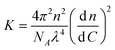
We use light scattering and small-angle X-ray scattering to obtain insight in the shape and size of the scattering objects as a function of charge ratio. To express the ratio of positive to negative charges we define a charge composition variable:²⁴which is the ratio between the concentration of positively chargeable groups on the polymers, [+], and the total concentration of chargeable groups on the polymers, [+] + [−]. f ⁺ is easily computed from the polymer characterization of groups, since we are dealing here with two strongly charged polyelectrolyte moieties. In this study we investigate the influence of charge ratio for several concentrations; dilute samples at 0.5wt%, and more concentrated samples at 5, 10, 15 and 20wt%. The charge ratio f ⁺ was varied, while keeping the total polymer weight concentration fixed. This means that the concentrations of both components change when changing f ⁺. An example for the 20wt% sample is given in Table 1.

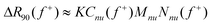
The scattered light intensity is used to compute the excess Rayleigh ratio at a scattering angle of 90°, ΔR₉₀, using eqn (2).^47,48

where I₉₀ is the scattered light intensity of the sample at a scattering angle of 90°, I_bg is the background scattering including solvent scattering and monomer scattering, I_tol is the reference scattering intensity of toluene at 90°, n = 1.3365 is the refractive index of the solvent,⁴⁹n_tol = 1.4961 is the refractive index of toluene⁴⁹ and R_tol = 2.1 × 10⁻³ m⁻¹ is the Rayleigh ratio of toluene at 90° for λ = 532 nm.⁵⁰ The value for I_bg(f ⁺) for each charge ratio is obtained by a linear interpolation of the scattered light intensities between the two extremes of the charge ratio, i.e. f ⁺ = 0.0 and f ⁺ = 1.0, see supporting information. This means that we subtract the maximum possible level of scattering not originating from aggregates, which is an overestimation of the real situation. However, this error is small, because the background scattering is much lower than the scattering of the sample, for most charge compositions. Hence, the reported values for the excess Rayleigh ratio originate from co-assembled structures only.

The excess Rayleigh ratio and average hydrodynamic radius for 0.5wt% solutions are displayed in Fig. 1. In the direction of increasing f ⁺, we initially see a modest increase of the excess Rayleigh ratio as well as the hydrodynamic radius, indicative of the formation of small scattering objects. Such objects have been named ‘soluble complexes’ in the past.^17,24,34 Upon approaching charge stoichiometry, we see a steep increase in the excess Rayleigh ratio and in the hydrodynamic radius. This increase can be attributed to the formation of ‘free’ micelles. These micelles have a polyelectrolyte complex core, consisting of the charged end-blocks of the triblock copolymer and the oppositely charged homopolymer. The polyelectrolyte complex core is stabilized by a corona of looped middle-blocks, since bridge formation is unlikely at these low concentrations. The micelles at charge stoichiometric conditions are named flowerlike polyelectrolyte complex micelles, since the looped middle-blocks represent the petals of a flower in a two dimensional representation of the micelles, see Fig. 9.^14,35 For the excess positive charge side of Fig. 1, f ⁺ > 0.5, the excess Rayleigh ratio decreases, but the drop is not as strong as on the excess negative charge side. The hydrodynamic radius of the scattering objects decreases somewhat compared to the 1 : 1 charge ratio, but the objects maintain a hydrodynamic radius that is in the micellar range of 15–25 nm. Clearly, the light scattering results show asymmetry as a function of charge ratio.

Fig. 1 Excess Rayleigh ratio (ΔR₉₀, ♦, left axis) and hydrodynamic radius (R_h, ◊, right axis), as a function of charge stoichiometry, f ⁺. Samples are prepared by direct mixing, and have been given time to equilibrate. Total polymer concentrations are 0.5wt% for all samples.

Such pronounced asymmetry has been observed only once for polyelectrolyte complex micelles based on diblock copolymers.⁵¹ On the contrary, there are many reports showing more symmetric profiles.^17,24–29 A similar trend in the hydrodynamic radius as in Fig. 1 was observed in a previous study with other triblock copolymers.³⁵ Both results indicate that in the case of an excess of the triblock copolymer, objects of micellar size can be tolerated in solution.

To further investigate the light scattering results, we have to make some assumptions about the origin of the scattering. The excess Rayleigh ratio is related to the weight concentration (C), the composition dependent mass (M(f ⁺)) and shape of the scattering objects, and the interaction between the scattering objects:

where P(q) is the particle form factor, S(q) is the structure factor and K is the optical constant defined as:where n = 1.3365 is the refractive index of the solvent,⁴⁹N_A is Avogadro's number, λ = 532 nm is the wavelength of the light and is the estimated refractive index increment, see supporting information. If we assume that the refractive index increment is independent of the overall stoichiometry,⁵² we find a value for the optical constant of K = 8.97 × 10⁻⁶ m² mol kg⁻².

We furthermore assume that P(q) ≈ 1 (since qR_h ≤ 0.5) and that the 0.5wt% solutions are dilute enough so that S(q) ≈ 1. The values for the excess Rayleigh ratio given in Fig. 1 are therefore proportional to the product of the weight concentration and the mass of the scattering objects.

We can now consider two extreme cases for the composition of the scattering objects: A) All polymers in solution are present in aggregates and thus contribute to the excess scattering. Since the overall concentration is equal in all samples, we can attribute the increase and decrease of the excess Rayleigh ratio to an increase and decrease in the mass of the aggregates. A consequence of this hypothesis is that all the excess charge is present on the aggregates themselves. B) The aggregates are electroneutral and the excess charge is present as free polymers in solution. In this case the increase and decrease in excess Rayleigh ratio originate from changes in weight concentration as well as changes in mass of the aggregates.

The real situation is probably somewhere in between these two extreme cases. However, we argue that the second case is closer to reality than the first, for four reasons: i) From a systematic study on polyelectrolyte-protein complexes, it has been shown that the charge ratio inside such a complex is close to stoichiometric, independent of the overall mixing ratio.³⁰ This implies that the excess charge is present in solution as free polymers. ii) For case A, the decrease in scattered light intensity observed for f⁺ > 0.5 in Fig. 1 must be caused by a decrease in the mass of the scattering objects. This is in disagreement with our observations shown in the same figure that the size of the scattering objects remains approximately constant for f ⁺ ≥ 0.5. iii) In case A all the polymers are present in aggregates, which means sacrificing a lot of translational entropy of the polymers. iv) Aggregates with excess charge are unfavourable because of electrostatic repulsion. The electrostatic energy needed to incorporate one extra charge is eΨ_d with Ψ_d the surface potential of the micellar core. This should not be much larger than the thermal energy kT, so that Ψ_d cannot be much more than 25 mV. From this we estimate the maximum surface charge σ ≈ εκΨ_d ≈ 0.05 C m⁻², with κ the inverse Debye screening length. Taking the surface area of the micellar core as a few hundred nm², this means that at most 1–5 extra triblock copolymers, or 1–2 extra homopolymers, can be incorporated per polyelectrolyte complex. As we will see below, this number is small compared to the overall aggregation number, so that the relative deviation from stoichiometry is small. Larger deviations from stoichiometry would require the incorporation of counterions into the polyelectrolyte complex core to compensate the excess charge, which would lead to a large loss of counterion entropy.

More detailed theoretical calculations by Shklovskii et al. and Rubinstein et al. substantiate our arguments in favour of case B, showing that a coexistence of neutral polyelectrolyte complexes and charged aggregates is more favourable than distributing all charges evenly over all complexes.^53,54

Based on these arguments, we propose that the relative deviations from the stoichiometric ratio in the polyelectrolyte complex core are small, and that most of the excess polymeric charge resides as free polymers in the solution. This means that for the calculation of the mass of the scattering objects it is reasonable to assume that all charges in the polyelectrolyte complex core are compensated, so that it can be considered as composed of neutral units. To proceed, we define the smallest possible charge neutral unit that can be present in an aggregate, which is one triblock copolymer exactly neutralized by oppositely charged homopolymer. Such a single neutralized unit is merely a convenient calculation aid; it does not really exist in our system, because there is a significant mismatch between the number of charges in one triblock copolymer and one homopolymer. Hence, we only use it for estimating the mass of our aggregates, where we assume that the charge mismatch averages out in the polyelectrolyte complex. The corresponding molar mass of such a neutralized unit is M_nu ≈ 41.1 kg mol⁻¹. The weight concentration of neutralized units present in solution varies per charge ratio and can be calculated taking into account the charge concentration of the minority species, thereby assuming that all of the minority species ends up in aggregates. The weight concentration of neutralized units, relative to the maximum weight concentration of neutralized units at charge stoichiometry, can be found in Table 1 and is shown graphically in the supporting information.

We can now rewrite eqn (3) to:

where C_nu(f ⁺) is the known weight concentration of neutralized units and N_nu(f ⁺) is the number of neutralized units per aggregate. Since all other values are known, we can easily estimate the number of neutralized units as a function of charge ratio from eqn (5). The results are shown in Fig. 2. Taking only C_nu as the weight concentration of aggregates may be an underestimation, because it does not include the possible excess polymers in the core. Therefore the values shown in Fig. 2 are an upper limit. The real number of neutralized units will be slightly lower, especially far way from f ⁺ = 0.5. We estimate the uncertainties in the calculated values to be in the order of 20%.

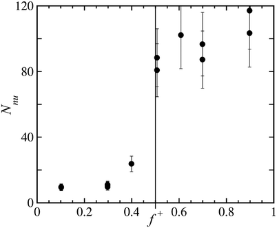Fig. 2 Estimate of the average number of neutralized units per aggregate, N_nu, as a function of charge ratio f ⁺. The error bars indicate the estimated degree of accuracy of ±20%.

Fig. 2 shows that for values of f ⁺ < 0.5, the number of neutralized units per scattering object is rather low, which is in agreement with the dynamic light scattering results showing objects of relatively small hydrodynamic radius. Upon approaching the charge stoichiometric ratio, there is a sudden increase in the number of neutralized units per aggregate, indicative of the formation of flowerlike micelles at f ⁺ = 0.5. The steep increase of the excess Rayleigh ratio for 0.3 ≤ f ⁺ ≤ 0.5 in Fig. 1, can thus be explained by an increase in both the mass per scattering object and the weight concentration of scattering objects. For values of f ⁺ ≥ 0.5, the weight concentration of scattering objects decreases, because C_nu decreases, but at the same time the mass per scattering object increases, see Fig. 2. This increase in mass per scattering object is the origin of the asymmetric shape of the excess Rayleigh ratio in Fig. 1. Apparently the micelles can become more massive at excess positive charge conditions. One possible way by which this happens is by the detachment of charged blocks from the core and concomitant unfolding of loops in the corona, and the subsequent replacement of the detached blocks by new triblock copolymers to maintain charge neutrality in the core. In this way, the polyelectrolyte complex core composition does not change, while at the same time the mass of the micelle increases, see Fig. 9. This exchange mechanism, where one looped triblock copolymer is exchanged for two triblock copolymers having one end in the polyelectrolyte core and one end free in solution, is plausible for the following reasons: i) the triblock copolymer end-block is hydrophilic; ii) the polyelectrolyte complex core can stay close to electroneutral; iii) the excess charge that accumulates in the corona can be spread over periphery of the corona, because the chains are still mobile, to minimize the charge density in the corona; iv) the relatively high salt concentration used in this study causes only short ranged electrostatic repulsion, in the order of 1 nm, and facilitates the exchange of polyelectrolyte end-blocks.

We performed small-angle X-ray scattering measurements to further investigate the shape of the scattering objects and their interactions. Eqn (3) also holds for X-ray scattering, provided that we take into account the different contrast for X-rays and the different magnitudes of the wave vectors q. The scattered intensity is now expressed as I(q, f ⁺) instead of the excess Rayleigh ratio in the case of light scattering. The scattering curves for charge compositions of f ⁺ = 0.0 to f ⁺ = 1.0 are shown in Fig. 3.

Fig. 3 SAXS curves for 0.5wt% total polymer concentration. Only 30% of the data points are shown. Symbols correspond to charge ratios as indicated in the graph.

In this figure we have also included 0.5wt% polymer solutions of both pure components, namely homopolymer only (f ⁺ = 0) and triblock copolymer only (f ⁺ = 1). We can now see the difference between the X-ray contrast of the two polymers. Clearly, the homopolymer has a higher scattering contrast than the triblock copolymer, which is probably due to the presence of the sulfur atom in the sulfonate moiety.

Rather strikingly, we see that almost all curves in Fig. 3 show a weak maximum at lower q-values. Only the f ⁺ = 0.9 and f ⁺ = 1.0 curves do not show a maximum. The curve of the f ⁺ = 0.9 sample has a somewhat peculiar shape, without a ‘plateau’ at low q. This shape would be difficult to explain and may be an experimental artefact. The weak maxima are indicative for interactions between the scattering objects. Apparently a concentration of 0.5wt% is not dilute enough to rule out interactions. Even the homopolymer solution shows signs of a repulsive interaction. The interaction must be predominantly of steric origin, since the electrostatic interactions are only short ranged at a salt concentration of 0.35 M. Considering the formation of complexes, we can see that the curves for f ⁺ = 0.1 and f ⁺ = 0.3 nearly overlap, indicating that a similar number of scattering objects of similar shape and size are present in solution. The curves of f ⁺ = 0.5 and f ⁺ = 0.7 can be clearly distinguished from the other curves, having a relatively high scattered intensity at low-q values, and a stronger q-dependence at higher q values. The shape of both curves is rather similar, the main difference being that the scattering of the f ⁺ = 0.7 curve is somewhat lower than for the 1 : 1 charge ratio, indicating that there are fewer scattering objects in solution.

None of the curves in Fig. 3 show form-factor minima, suggesting that the scattering objects are relatively polydisperse, even at 1 : 1 charge ratio. From previous reports it is known that salt concentration has a profound influence on the polydispersity of polyelectrolyte complex micelles.^17,35,55,56 However, lowering the salt concentration to a minimum of 10 mM KCl, does not change the SAXS curve significantly, see supporting information. As shown by Spruijt and coworkers, we should not consider the absolute salt concentration as measure for the driving force for complex formation, but rather consider how close we are to the critical salt concentration.⁵⁷ The latter is defined as the salt concentration where the driving force to form a complex between two oppositely charged homopolymers of equal length vanishes. The critical salt concentration for the currently investigated combination of polyelectrolytes is a factor of three lower than for the combination studied in previous papers.^14,20,35 A lower driving force for complex formation leads to less well-defined objects, which explains the polydisperse nature of the complexes studied in this paper.

To see if the asymmetry in the excess Rayleigh ratio is also present in the X-ray scattering, we plot the values for I(0.1) as function of charge ratio in Fig. 4. We assume here that this low-q scattering depends only on the weight concentration of scattering objects and the mass per scattering object. The shape of the I(0.1) graph is very similar to the one in Fig. 1, both showing asymmetry as a function of charge composition. Note that the difference in I(0.1) between f ⁺ = 0.5 and f ⁺ = 0.7 is relatively small, considering the relatively big difference in concentration of neutralized units in solution, see Table 1. This means that the scattering at f ⁺ = 0.7 is higher than expected based on the weight concentration of scattering objects. This can only be explained by an increase in mass per scattering object at f ⁺ = 0.7, which is in agreement with the results of Fig. 2.

Fig. 4 Values for I(0.1) from the scattering curves (●, left axis), and minus the slope of the SAXS curves at high-q (○, right axis), as a function of charge ratio f ⁺, for the 0.5wt% sample.

Also the slopes of the SAXS curves at high q in Fig. 3 change as a function of charge stoichiometry. We have analysed the slopes for q ≥ 0.3 nm⁻¹ for the different charge ratios, and the result can be found in Fig. 4. Again we see an asymmetric shape, with a maximum at 1 : 1 charge ratio. The higher the slope, the sharper is the interface of the scattering object. In other words, the scattering objects are the least ‘fluffy’ at 1 : 1 charge ratio.

Scattering of concentrated solutions

We have measured SAXS patterns also for more concentrated samples of 5wt%, 10wt%, 15wt% and 20wt%, to investigate how the scattering objects interact with each other. Fig. 5 shows the result of the 20wt% samples. The scattering curves of 5wt%, 10wt% and 15wt% can be found in the supporting information.

Fig. 5 SAXS curves for 20wt% total polymer concentration. Only 30% of the data points are shown. Symbols correspond to charge ratios as indicated in the graph.

The scattering curves of both the homopolymer only and triblock copolymer only solutions are independent of q, indicating that the solutions are above the overlap concentration and that the typical length scale is beyond the limit of our explored q-range. The scattering of the f ⁺ = 0.1 sample is somewhat higher than the f ⁺ = 0 sample, caused by the formation of small objects; we can just see the influence of the form factor for the highest q-values. Apparently the volume fraction of these small scattering objects is low, since there is no sign of interactions in the curve. All other investigated samples do show a structure peak. This peak is most pronounced in the 1 : 1 charge ratio sample.

In general, the position of the maximum in the scattered intensity corresponds to a typical length scale, meaning that the centers of the scattering objects are frequently found at a distance of apart from each other. A true peak in the scattered intensity can be seen in the curves around charge stoichiometry, i.e. for the values of f ⁺ = 0.3, f ⁺ = 0.5 and f ⁺ = 0.7. We have computed the values for D for these three charge compositions and for the four different concentrations investigated, see Fig. 6a. The distance between the centers of the scattering objects decreases with increasing concentration, as expected. D decreases approximately with the cubic root of the concentration for f ⁺ = 0.5 and f ⁺ = 0.7, meaning that the volume fraction of the scatterers increases linearly with concentration. Note that the values at 5wt% are less accurate than the other values, since no clear maximum can be seen in the scattering curves, see supporting information. Extrapolating the f ⁺ = 0.7 data fit to a concentration of 0.5wt% yields a typical length scale of D ≈ 75 nm, corresponding to a q_peak ≈ 0.08 nm⁻¹. This is indeed the value where we start to see interactions between the scattering objects, in the form of a weak maximum, for the f ⁺ = 0.7 samples, see Fig. 3.

Fig. 6 Qualitative measures for the degree of order in the different samples. (a) Typical distance between the centers of the scattering objects. The line is a power-law fit to the f ⁺ = 0.7 data, and scales as C^−0.3. (b) , as a function of weight concentration of neutralized units C_nu, for f⁺ = 0.3(♦), f ⁺ = 0.5 (○) and f ⁺ = 0.7 (×).

Comparing the results for different charge compositions, we see again that the samples of f ⁺ = 0.5 and f ⁺ = 0.7 are almost similar. D is lower for the f ⁺ = 0.3 sample, in agreement with the previous findings that the scattering objects at this charge ratio are considerably smaller.

A different qualitative measure for the degree of ordering in the sample is the ratio of the scattered intensity maximum and the scattered intensity at low q-values, . These values have been computed for the three different charge compositions and are plotted as a function of the concentration of neutralized units (see supporting information) in Fig. 6b.

The order in the samples increases with increasing concentration of neutralized units for the f ⁺ = 0.5 and the f ⁺ = 0.7 samples. For low concentrations, the ordering for the f ⁺ = 0.7 samples seems to be consistently higher than for the other samples. In other words, with the same amount of aggregated material the ordering is stronger in the f ⁺ = 0.7 samples. This may be caused by a longer ranged repulsion in these samples, or by an increased volume fraction with the same amount of aggregates. The latter implies that the density of the total aggregates is somewhat lower for f ⁺ = 0.5 conditions.

For higher concentrations of neutralized units, we see a pronounced increase in structure formation for the f ⁺ = 0.5 samples. This strong increase is caused by the combination of the attractive bridging interactions and the repulsion between the micellar coronas, which keeps the micelles at a preferred distance from each other.^14,35 The f ⁺ = 0.7 samples show a similar upturn in structure formation. Unfortunately, we cannot determine whether this would keep increasing, as C_nu does not become higher than 11wt% in the f ⁺ = 0.7 samples. The ordering is least in the f ⁺ = 0.3 samples. Apparently, the volume fraction of these smaller aggregates is too low to induce pronounced ordering, which would mean that the density of these aggregates is higher than for f ⁺ ≥ 0.5 conditions. Another possible explanation for the lack of ordering in this sample is that the particles are softer.

SAXS data fitting

Although there are no form- and structure factors available describing the shape and interactions of non-stoichiometric polyelectrolyte complex micelles, we assume that a core-shell model does reasonably well to get an idea of the size of the scattering objects. Interactions between particles may be described by the hard-sphere model, as a first approximation. We use these simple models, which were shown to work well for flowerlike micelles of stoichiometric charge ratio,^14,35 to get an idea of the relevant sizes and the range of interactions. The resulting fits and fitting parameters can be found in the supporting information, as well as the fitted values for I(0) for both 0.5wt% and 20wt%, which show similar asymmetry as Fig. 1 and 4. Here we show the results for the fitted radii R_core, R_shell and total aggregate radius R_agg = R_core + R_shell, the effective hard sphere radius, R_HS, and the effective volume fraction of hard spheres, ϕ.

Fig. 7 shows the results for the several radii obtained by model fitting the SAXS data in dilute (0.5wt%, Fig. 7a) and concentrated (20wt%, Fig. 7b) samples. Note that the 0.5wt% SAXS curves could be satisfactorily fitted by applying a form factor fit only, see supporting information. From Fig. 7a we can see that, in the dilute samples, R_shell > R_core for all charge compositions. The shell thickness increases with increasing f ⁺, whereas the core radius seems to have a maximum around f ⁺ = 0.5. There is a steep increase in shell radius from f ⁺ = 0.7 to f ⁺ = 0.9, which fits the hypothesis that the loops in the corona unfold, sticking one charged end-block into the solution. Overall, the SAXS fitting results are in agreement with the dynamic light scattering data of Fig. 1. For excess negative charge we have smaller scattering objects of approximately 10 nm, and for excess positive charge we have bigger scattering objects of 15–20 nm. However, the hydrodynamic radius from Fig. 1 seems to be more or less constant for excess positive charge, and does not display this ‘jump’ for f ⁺ = 0.9.

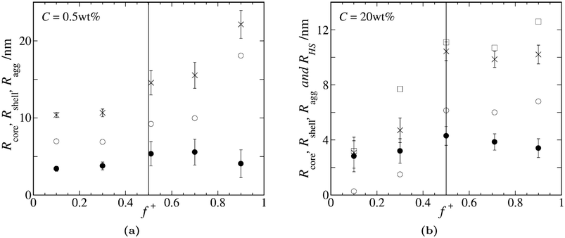Fig. 7 Graphs show the different radii as obtained from model fitting the SAXS data. Symbols indicate different radii: R_core (●), R_shell (○), R_agg (×) and R_HS (□). Error bars correspond to the relative standard deviation of R_core, as obtained by the fit. (a) Radii from fitting the 0.5wt% data. (b) Radii from fitting the 20wt% data.

Model fitting of the 20wt% samples results in smaller micelles than in the diluted samples, see Fig. 7b. The core radius seems to exhibit again a maximum around f ⁺ = 0.5. The shell seems to be almost absent in the f ⁺ = 0.1 sample, after which its thickness increases towards a constant value for values f ⁺ ≥ 0.5. The hard-sphere radius R_HS is always slightly bigger than the total aggregate radius R_agg, and corresponds quite well to half of the average center-to-center distance D, as shown in Fig. 6a. From the structure factor fit we obtain the hard-sphere radius and the effective volume fraction of hard-spheres. The fitted values are displayed in Fig. 8 and show asymmetry, similar to the experimental results of Fig. 1 and 4. That the volume fraction exhibits a maximum at 1 : 1 charge ratio is obvious, since at this point C_nu is highest. Since ϕ is approximately linear with concentration, we can correct for the concentration by dividing the volume fraction by the relative amount of neutralized units from Table 1. What we obtain is a measure for the average volume per neutralized unit, see Fig. 8. The increase observed in this figure must mean that the average density of the scattering objects decreases for excess positive charge, as compared to the f ⁺ = 0.5 sample. This is in agreement with the results in Fig. 6b for the f ⁺ = 0.7 samples.

Fig. 8 Effective volume fraction of hard-spheres as a function of charge ratio (♦, left axis) and the volume fraction corrected for the relative amount of neutralized units in solution (□, right axis).

Structural summary

Overseeing all the results from the scattering experiments, the following picture emerges, which is summarized in Fig. 9. For dilute solutions at charge stoichiometric conditions, f ⁺ = 0.5, we obtain relatively polydisperse spherical flowerlike micelles of radius 15–20 nm. The core is at the maximum of its size and density at these conditions.

Fig. 9 Several illustrations showing the different situations for excess negative charge, charge stoichiometry and excess positive charge, for two concentration regimes, dilute and concentrated.

For dilute solutions with excess negative charge, f ⁺ < 0.5, we assume that all triblock copolymers bind to the negatively charged homopolymer. Since there is an excess of homopolymer, it is likely that smaller aggregates are formed, composed of a few neutralized units, see the upper-left part of Fig. 9. These aggregates must carry some excess negative charge that prevents them from further aggregation into bigger clusters. As discussed above, even a relatively small excess of the negatively charged homopolymer in terms of mass could already lead to large surface potential. Such small aggregates are typically called ‘soluble complexes’.^17,24 Probably most excess negative charge is present in solution in the form of unbound homopolymer. Upon approaching the charge stoichiometric point, the soluble complexes grow in size, thereby decreasing the excess charge in the complex, until we have a maximum amount of aggregated material in the form of neutral flowerlike micelles.

The situation is somewhat different for the excess positive side of the composition diagram, where f ⁺ > 0.5. All data suggest that we still have objects of micellar size, probably with even higher aggregation numbers per object than in the 1 : 1 charge ratio situation. Such behaviour has not been observed before for polyelectrolyte complex micelles prepared from (combinations of) diblock copolymers. Therefore this behaviour must be explained by the properties of the triblock copolymer. For excess positive charge conditions, triblock copolymers have the choice to put both end-blocks in the polyelectrolyte complex core, or to put only one end-block in the core and leave the other end-block free in solution. The latter option is a convenient way of dealing with the excess positive charge; the polyelectrolyte complex core can stay close to electroneutral, while the excess charge is spread out over the periphery of the corona. With increasing f ⁺, the amount of loops will decrease and the amount of free end-blocks will increase, see the upper-right part of Fig. 9. The strong increase of the shell radius for f ⁺ = 0.9 might be caused by the enhanced stretching of the corona chains, either because of crowding or to minimize the charge density at the exterior of the corona. The more stretched the coronas become, the softer and less well defined the micelles become. If all triblock copolymers have adapted a stretched conformation, instead of the looped conformation at f ⁺ = 0.5, while keeping the total amount of charges in the core equal, the aggregation number has to increase by approximately a factor of 1.5. This is in good agreement with Fig. 2 and 8.

For the concentrated samples at charge stoichiometry the flowerlike micelles become somewhat smaller. With increasing concentration, the flowerlike micelles get closer and closer to each other, until the average distance between the micelles approaches the value of twice the hard-sphere radius.

Concentrated solutions of excess negative charge lead to significantly smaller soluble complexes as compared to the dilute conditions. The volume fraction of soluble complexes in the investigated samples is too low to cause strong ordering. However, we do see a relatively big difference between the aggregate radius and the hard-sphere radius at f ⁺ = 0.3. It is not likely that this is caused by a long ranged electrostatic repulsion between the negatively charged complexes, because the Debye screening length is in the order of 1 nm at 0.35 M KCl.

Concentrated solutions of excess positive charge also show a decrease in micellar size as compared to the dilute situation. However, the radius of the aggregates is approximately constant for excess positive charge conditions and high concentrations, contrary to the increase in radius for these conditions in the dilute samples, see Fig. 7. Apparently, the presence of the other micelles limits the corona's ability to stretch. The ordering in these samples might be even more pronounced than in the 1 : 1 charge ratio samples, for equal weight concentrations of neutralized units. This is because the aggregates take up more volume for equal concentrations of neutralized units at excess positive charge conditions. The latter implies that the average density of the aggregates decreases with increasing f ⁺.

Rheometry of concentrated solutions

Since our triblock copolymers have two ‘sticky’ end-blocks, it is possible for a triblock copolymer to stick both end-blocks in a different micellar core, forming a bridge. The average number of bridges per micelle depends predominantly on the average distance between the micelles, which is in turn determined by the concentration of neutralized units. If the concentration of micelles is high enough, a percolating path of interconnected micelles can be formed, leading to physical gel formation. For triblock copolymers with a PEO(10k) middle-block, the concentration of neutralized units where a percolating network can be formed is between 4wt% and 8wt%.^14,35 The microstructure is reflected in the mechanical properties of a gel, which can be probed experimentally by measuring the elastic modulus, G. The elastic modulus of a polymeric network is related to the microstructure by:

G ≃ νkT (6)

where ν is the number density of elastically active chains, k is Boltzmann's constant and T is the absolute temperature. Hence, the higher the number density of elastically active chains, the higher the elastic modulus. The elastic modulus can be obtained from a rheological frequency sweep experiment, if one can measure a high-frequency plateau of the storage modulus, where G′(ω) = constant. The storage modulus can only be measured if the bridges in the material can be regarded as ‘frozen’ on the time scale of the applied deformation, i.e. when ω⁻¹ < τ, where τ is the mechanical relaxation time of the sample. The relaxation time can be approximated as the inverse of the cross-over frequency, where G′ = G′′. Hence, whether a plateau modulus can be measured depends on the relaxation time of the sample, and the dynamic range of the rheometer.

Fig. 10 shows the results of frequency sweep measurements in which we varied either the concentration or the charge ratio. From Fig. 10a we can see that the cross-over frequency, and thus the relaxation time, is a weak function of concentration. Between the 10wt% and 20wt% the cross-over frequency shifts from 400 rad s⁻¹ to 250 rad s⁻¹, corresponding to a relaxation time in the order of a few milliseconds. The shift in relaxation time from 5wt% to 10wt% is caused by further development of the network, which is very open at 5wt%. In open networks, the probability to form so called ‘super-chains’ is higher than in more dense networks. According to Annable and coworkers, super-chains can relax stresses more rapidly than single bridges, which possibly explains the concentration dependence of the relaxation time for concentrations close to the gel concentration.²

Fig. 10 Results of frequency sweep measurements. (a) Frequency sweeps for fixed charge ratio of f ⁺ = 0.5, for different total polymer concentrations. (b) Frequency sweeps for fixed total polymer concentration of 20wt%, for different charge compositions. Storage moduli, G′, are indicated as filled symbols, loss moduli, G′′, are indicated as open symbols. The meaning of the symbols is explained in the graphs.

Fig. 10b shows that the relaxation time for the off-stoichiometric charge compositions is even shorter, making the relaxation time and plateau modulus impossible to assess with a conventional rheometer. Note that the values for the loss moduli in Fig. 10 are parallel, scaling as G′′ ∝ ω, which indicates Newtonian liquid-like behaviour over the measured frequency domain.

Since it is not possible to measure the plateau modulus for these systems, we investigate the shear viscosity. The viscosity reflects both the number of bridges in the sample and their relaxation dynamics. For a single relaxation time Maxwell liquid:

η ≃ Gτ (7)

The viscosity of the 20wt% samples is shown in Fig. 11 as a function of shear rate. There is a Newtonian plateau in the shear viscosity for low enough shear rates, in accordance with the frequency sweep experiments. The low-shear plateau value of the viscosity is referred to as the zero-shear viscosity, η₀. The 1 : 1 charge ratio sample shows the onset of shear thinning behaviour at shear rates between 10–100 s⁻¹, which is at somewhat lower shear rates than expected, given the mechanical relaxation time of a few milliseconds obtained by frequency sweep measurements.

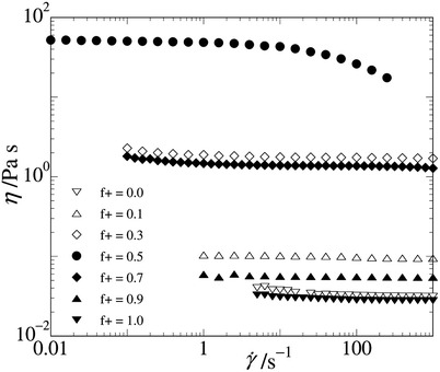Fig. 11 Flow curve for the 20wt% samples, for different charge compositions indicated in the graph.

In Fig. 12 we have plotted the values for η₀ as a function of charge ratio, and for different polymer concentrations, both on a linear scale (Fig. 12a) and on a logarithmic scale (Fig. 12b). In Fig. 12a we can see that for the 10wt%–20wt% samples there is a very pronounced peak in the zero-shear viscosity for charge stoichiometric conditions. The difference in zero-shear viscosity going from 10wt% to 20wt% is almost exclusively caused by an increase in the number density of active chains in the transient network, because there is little difference in relaxation time for the 1 : 1 charge ratio samples of 10–20wt%, see Fig. 10a.

Fig. 12 Zero-shear viscosity as a function of charge ratio, for different concentrations. Symbols correspond to concentrations, as displayed in the legend. The lines in (a) and (b) are fits to the data, and are meant to guide the eye.

On the logarithmic y-axis in Fig. 12b, we can see that the one-component polymer solutions show the lowest viscosity, approximately 10–30 times the viscosity of water. We can also see that the effect of charge ratio on the zero-shear viscosity is stronger in the 10–20wt% samples than in the 5wt% samples. In the case of the more concentrated solutions, we see that the zero-shear viscosity increases almost exponentially with decreasing excess charge, reaching the maximum value at f ⁺ = 0.5.

A close inspection of Fig. 12b shows that the viscosity as function of charge ratio is not precisely symmetric. The viscosities of solutions with excess negative charge are higher than solutions with the same excess positive charge. Even though the effect is not very pronounced, it is consistent for all concentrations. This asymmetry can be explained by the relative weight concentration of neutralized units in the samples. As can be seen in Table 1, the excess negative side has relatively more neutralized units than the excess positive side, for equal distance from the charge stoichiometric point. More neutralized units allows for more structure formation in the samples which leads to a higher viscosity.

Can we deduce from the data presented whether transient network formation is possible also at off-stoichiometric conditions? To answer this question it is convenient to replot the data in Fig. 12, as a function of the concentration of neutralized units. This is done in Fig. 13, both on a linear scale (Fig. 13a) and on a logarithmic scale (Fig. 13b). Again we can see the dramatic increase in viscosity for the 1 : 1 charge ratio samples in Fig. 13a. This strong increase is characteristic for the build-up of a percolating network beyond the percolation threshold of C_gel ≈ 8wt%. This value is approximately two times the overlap concentration of the middle-block PEO(10k). The strong increase in viscosity is related to the strong increase in structural order, as presented in Fig. 6b. It is however remarkable that the structural order is almost similar for the f ⁺ = 0.5 and f ⁺ = 0.7 samples, see Fig. 6b, whereas the viscosity in the f ⁺ = 0.7 samples is clearly lower than in the f ⁺ = 0.5 samples, for C_nu ≥ 8wt%. This means that it is not the structural order in the sample, but the bridge formation between the micelles that causes the increase in viscosity for the 1 : 1 charge ratio samples.

Fig. 13 Zero-shear viscosity as a function of weight concentration of neutralized units, for different charge compositions. Symbols correspond to charge compositions, as displayed in the legend. The lines in (b) are guides to the eye.

Fig. 13b displays the increase in zero-shear viscosity as a function of concentration of neutralized units on a logarithmic scale. Somewhat to our surprise, all data points below C_gel collapse onto a master-curve, showing an exponential increase of the zero-shear viscosity with the concentration of neutralized units. The higher the concentration of neutralized units is, the more difficult it is for the aggregates to slide past each other and, hence, the higher is the resistance to flow. The size, or excess charge of the aggregates seems to be of little influence to the viscosity.

An exponential increase of the viscosity has been reported in rheological experiments on other soft colloidal systems such as emulsions⁵⁸ and polymer solutions.^59,60 It has also been predicted by Semenov et al., who showed that the relaxation time, and thus the viscosity, of a transient network of triblock copolymers should increase exponentially with concentration, in a concentration regime just above the overlap concentration.⁶¹ This may well be the concentration regime we are investigating here.

For higher concentrations we see that the viscosity keeps increasing for the samples of f ⁺ = 0.3, f ⁺ = 0.5 and f ⁺ = 0.7. The increase is most clearly observed for the f ⁺ = 0.5 sample, where we see a change in slope for the increase of the viscosity at C_nu ≈ 10wt%. Since the relaxation time is approximately constant in this concentration regime, the increase in viscosity for this sample is mainly caused by the increase in the number of bridges between the micelles. More details about the gel properties at charge stoichiometry can be found elsewhere.^14,35 The viscosities of the f ⁺ = 0.3 and f ⁺ = 0.7 samples are approximately an order of magnitude lower than the f ⁺ = 0.5 samples, and the change in slope seems to be present at somewhat lower concentrations of neutralized units. The decreased viscosity, as compared to the f ⁺ = 0.5 sample, can be caused either by suppressed bridge formation or by a lower relaxation time.

It is likely that bridge formation is suppressed in the excess positive charge samples. In this case the polyelectrolyte complex cores of the micelles remain close to electroneutral. Hence, there is no driving force for association of the free end-blocks. For entropic reasons, these chain-ends want to stay ‘free’ in solution and thus the free end-blocks act as network stoppers, see bottom-right part of Fig. 9. The situation might be different for the soluble complexes at excess negative charge conditions. The soluble complexes should still be able to function as nodes in a network, given that C_nu ≥ 8wt%. However, the soluble complexes might be too small and/or too dense and therefore too dilute to come close enough to each other to enable bridge formation. Indeed the size of a soluble complex is relatively small compared to the distance between the micelles, see Fig. 6a and 7b. Another possibility is that transient network formation is possible, but that the dynamics of a negatively overcharged network are much faster than at charge stoichiometric conditions. One can imagine that a polyelectrolyte complex carrying excess charges is more likely to break up than a neutral polyelectrolyte complex. Probably suppressed bridge formation and enhanced dynamics are both of importance, but based on the current data we cannot be conclusive about what happens on the molecular level of concentrated solutions of soluble complexes. The bottom-left part of Fig. 9 gives an illustration of this situation.

Conclusions

We have studied the influence of charge composition on the formation of polyelectrolyte complex networks consisting of a negatively charged homopolymer and an ABA triblock copolymer, in which the A blocks carry positive charges. Scattering studies were performed on dilute as well as concentrated samples, rheological studies were performed on the concentrated samples only. Based on the experimental results, the following picture emerges.

For excess negative charge conditions, the triblock copolymer and homopolymer associate into small aggregates of radius 5–10 nm, called soluble complexes. These soluble complexes carry excess negative charge on the polyelectrolyte complex itself, combined with free homopolymer in solution. In concentrated solutions of these soluble complexes, the viscosity is significantly lower than in the charge stoichiometric situation. The lower viscosity is caused either by enhanced dynamics of the charged polyelectrolyte complex moieties, or by the lack of network formation due the relatively larger distance between the soluble complexes, making bridge formation unlikely.

At charge stoichiometry, neutral flowerlike micelles of radius 15–20 nm are present in solution. The flowerlike micelles are best defined at this 1 : 1 charge ratio. At sufficiently high concentrations these flowerlike micelles become interconnected, leading to a transient network.

Excess positive charge conditions lead again to a different situation. Objects of micellar size are present in solution. This is a unique feature of our triblock copolymer system, and does not occur in diblock copolymer systems. Polyelectrolyte complex micelles carrying excess positive charge can be tolerated in solution because the triblock copolymers can localize the excess positive charge on the periphery of the micellar corona, rather than in the micellar core. This enables the existence of a neutral polyelectrolyte complex core, even for excess positive charge conditions. The larger the excess charge in the system, the more free end-blocks protrude into solution. This also leads to the stretching of the triblock copolymer chains in the corona. In concentrated solutions, the micelles shrink considerably leading to a somewhat denser corona. The free end-blocks act as network stoppers, since there is no driving force for these free end-blocks to associate with a neutral polyelectrolyte complex core. Bridge formation between the micelles is therefore suppressed, leading to significantly lower viscosities as compared to charge stoichiometric conditions. Fig. 9 summarizes the various states of the system in pictorial form.

An inverse description should hold for the inverse system, i.e. a positively charged homopolymer combined with a triblock copolymer carrying negatively charged end-blocks. Whether similar behaviour can be seen in other systems, will predominantly depend on the association strength of the used polyelectrolyte pair and the salt concentration in solution. We believe that with the right combination of parameters, similar behaviour must show up in experiments with alike systems.

The possibility to vary the charge ratio is a unique feature of two-component polyelectrolyte systems. The influence of this parameter on the transient network formation has now been studied for the first time. Changing the charge ratio to off-stoichiometric conditions creates opportunities for further fine-tuning of the transient network properties, and therewith the mechanical properties of this two-component rheology modifier.

Acknowledgements

The Netherlands Organization for Scientific Research (NWO) is gratefully acknowledged for providing beam-time at the Dutch-Belgium Beamline (DUBBLE), BM26. ML would like to thank the men at the AFSG workshop for designing and manufacturing a very convenient multi-capillary holder. In particular ML would like to thank his colleagues for the excellent team-work while obtaining the SAXS data. This research is funded by the Dutch Polymer Institute (DPI), project #657.

References

1. S. T. Milner and T. A. Witten, Macromolecules, 1992, 25, 5495–5503.
2. T. Annable, R. Buscall, R. Ettelaie and D. Whittlestone, J. Rheol., 1993, 37, 695–726.
3. R. D. Jenkins, D. R. Bassett, C. A. Silebi and M. S. Elaasser, J. Appl. Polym. Sci., 1995, 58, 209–230.
4. X. X. Meng and W. B. Russel, J. Rheol., 2006, 50, 189–205.
5. J. Sprakel, N. A. M. Besseling, M. A. Cohen Stuart and F. A. M. Leermakers, Eur. Phys. J. E, 2008, 25, 163–173.
6. J. Sprakel, E. Spruijt, M. A. Cohen Stuart, N. A. M. Besseling, M. P. Lettinga and J. van der Gucht, Soft Matter, 2008, 4, 1696–1705.
7. J. F. Berret, D. Calvet, A. Collet and M. Viguier, Curr. Opin. Colloid Interface Sci., 2003, 8, 296–306.
8. P. Kujawa, H. Watanabe, F. Tanaka and F. M. Winnik, Eur. Phys. J. E, 2005, 17, 129–137.
9. D. Mistry, T. Annable, X. F. Yuan and C. Booth, Langmuir, 2006, 22, 2986–2992.
10. R. Obeid, E. Maltseva, A. F. Thunemann, F. Tanaka and F. M. Winnik, Macromolecules, 2009, 42, 2204–2214.
11. C. Tsitsilianis, Soft Matter, 2010, 6, 2372–2388.
12. R. C. W. Liu, Y. Morishima and F. M. Winnik, Polym. J., 2002, 34, 340–346.
13. F. Bossard, V. Sfika and C. Tsitsilianis, Macromolecules, 2004, 37, 3899–3904.
14. M. Lemmers, J. Sprakel, I. K. Voets, J. van der Gucht and M. A. Cohen Stuart, Angewandte Chemie-International Edition, 2010, 49, 708–711.
15. A. Harada and K. Kataoka, Macromolecules, 1995, 28, 5294–5299.
16. A. V. Kabanov, T. K. Bronich, V. A. Kabanov, K. Yu and A. Eisenberg, Macromolecules, 1996, 29, 6797–6802.
17. M. A. Cohen Stuart, N. A. M. Besseling and R. G. Fokkink, Langmuir, 1998, 14, 6846–6849.
18. M. A. Cohen Stuart, B. Hofs, I. K. Voets and A. de Keizer, Curr. Opin. Colloid Interface Sci., 2005, 10, 30–36.
19. I. K. Voets, R. de Vries, R. Fokkink, J. Sprakel, R. P. May, A. de Keizer and M. A. Cohen Stuart, Eur. Phys. J. E, 2009, 30, 351–359.
20. J. van der Gucht, E. Spruijt, M. Lemmers and M. A. Cohen Stuart, J. Colloid Interface Sci., 2011, 361, 407–422.
21. I. K. Voets, A. de Keizer, P. de Waard, P. M. Frederik, P. H. H. Bomans, H. Schmalz, A. Walther, S. M. King, F. A. M. Leermakers and M. A. Cohen Stuart, Angew. Chem., Int. Ed., 2006, 45, 6673–6676.
22. Y. Yan, N. A. M. Besseling, A. de Keizer, A. T. M. Marcelis, M. Drechsler and M. A. Cohen Stuart, Angew. Chem., Int. Ed., 2007, 46, 1807–1809.
23. S. Lindhoud, R. de Vries, W. Norde and M. A. Cohen Stuart, Biomacromolecules, 2007, 8, 2219–2227.
24. S. van der Burgh, A. de Keizer and M. A. Cohen Stuart, Langmuir, 2004, 20, 1073–1084.
25. B. Hofs, I. K. Voets, A. de Keizer and M. A. Cohen Stuart, Phys. Chem. Chem. Phys., 2006, 8, 4242–4251.
26. B. Hofs, A. de Keizer and M. A. Cohen Stuart, J. Phys. Chem. B, 2007, 111, 5621–5627.
27. I. K. Voets, A. de Keizer, M. A. Cohen Stuart, J. Justynska and H. Schlaad, Macromolecules, 2007, 40, 2158–2164.
28. I. K. Voets, R. Fokkink, T. Hellweg, S. M. King, P. de Waard, A. de Keizer and M. A. Cohen Stuart, Soft Matter, 2009, 5, 999–1005.
29. S. Lindhoud, W. Norde and M. A. Cohen Stuart, J. Phys. Chem. B, 2009, 113, 5431–5439.
30. J. Gummel, F. Boue, B. Deme and F. Cousin, J. Phys. Chem. B, 2006, 110, 24837–24846.
31. H. V. Saether, H. K. Holme, G. Maurstald, O. Smidsrod and B. T. Stokke, Carbohydr. Polym., 2008, 74, 813–821.
32. M. Antonov, M. Mazzawi and P. L. Dubin, Biomacromolecules, 2010, 11, 51–59.
33. R. Chollakup, W. Smitthipong, C. D. Eisenbach and M. Tirrell, Macromolecules, 2010, 43, 2518–2528.
34. V. A. Kabanov and A. B. Zezin, Makromol. Chem., 1984, 6, 259–276.
35. M. Lemmers, I. K. Voets, M. A. Cohen Stuart and J. van der Gucht, Soft Matter, 2011, 7, 1378–1389.
36. K. Jankova, X. Y. Chen, J. Kops and W. Batsberg, Macromolecules, 1998, 31, 538–541.
37. J. M. Dust, Z. H. Fang and J. M. Harris, Macromolecules, 1990, 23, 3742–3746.
38. K. Jankova and J. Kops, J. Appl. Polym. Sci., 1994, 54, 1027–1032.
39. M. Kato, M. Kamigaito, M. Sawamoto and T. Higashimura, Macromolecules, 1995, 28, 1721–1723.
40. J. S. Wang and K. Matyjaszewski, Macromolecules, 1995, 28, 7901–7910.
41. Y. T. Li, S. P. Armes, X. P. Jin and S. P. Zhu, Macromolecules, 2003, 36, 8268–8275.
42. G. Masci, D. Bontempo, N. Tiso, M. Diociaiuti, L. Mannina, D. Capitani and V. Crescenzi, Macromolecules, 2004, 37, 4464–4473.
43. W. Bras, I. P. Dolbnya, D. Detollenaere, R. van Tol, M. Malfois, G. N. Greaves, A. J. Ryan and E. Heeley, J. Appl. Crystallogr., 2003, 36, 791–794.
44. S. Forster and C. Burger, Macromolecules, 1998, 31, 879–891.
45. S. Forster, A. Timmann, M. Konrad, C. Schellbach, A. Meyer, S. S. Funari, P. Mulvaney and R. Knott, J. Phys. Chem. B, 2005, 109, 1347–1360.
46. S. Forster, L. Apostol and W. Bras, J. Appl. Crystallogr., 2010, 43, 639–646.
47. G. Deželić, Pure Appl. Chem., 1970, 23, 327–354.
48. H. Lindner and O. Glatter, Part. Part. Syst. Charact., 2000, 17, 89–95.
49. D. R. Lide, CRC Handbook of Chemistry and Physics, CRC Press, Boca Raton, FL, 2005.
50. H. Wu, Chem. Phys., 2010, 367, 44–47.
51. J. F. Gohy, S. K. Varshney, S. Antoun and R. Jerome, Macromolecules, 2000, 33, 9298–9305.
52. I. K. Voets, PhD Thesis, 2008.
53. R. Zhang and B. T. Shklovskii, Phys. A, 2005, 352, 216–238.
54. N. P. Shusharina, E. B. Zhulina, A. V. Dobrynin and M. Rubinstein, Macromolecules, 2005, 38, 8870–8881.
55. Y. Yan, A. de Keizer, M. A. Cohen Stuart, M. Drechsler and N. A. M. Besseling, J. Phys. Chem. B, 2008, 112, 10908–10914.
56. J. Wang, A. de Keizer, R. Fokkink, Y. Yan, M. A. Cohen Stuart and J. van der Gucht, J. Phys. Chem. B, 2010, 114, 8313–8319.
57. E. Spruijt, J. Sprakel, M. A. Cohen Stuart and J. van der Gucht, Soft Matter, 2010, 6, 172–178.
58. C. G. Quintero, C. Noik, C. Dalmazzone and J. L. Grossiord, Rheol. Acta, 2008, 47, 417–424.
59. R. E. Whittier, D. W. Xu, J. H. van Zanten, D. J. Kiserow and G. W. Roberts, J. Appl. Polym. Sci., 2006, 99, 540–549.
60. E. Choppe, F. Puaud, T. Nicolai and L. Benyahia, Carbohydr. Polym., 2010, 82, 1228–1235.
61. A. N. Semenov, J. F. Joanny and A. R. Khokhlov, Macromolecules, 1995, 28, 1066–1075.

---

Footnote

† Electronic supplementary information (ESI) available. See DOI: 10.1039/c1sm06281f

---