Estimation of kinetic parameters from time-resolved fluorescence data: A compressed sensing approach

Abstract

The characterization of fluorescence kinetic measurements by a set of lifetimes and amplitudes is a well-known, ill-posed problem. The most effective approaches for dealing with this difficulty generally look for a regularized distribution of amplitudes on a predefined large grid of time constants. Here we argue that in the absence of any additional a priori knowledge on the underlying mechanism, the simplest solution of any complex kinetics is the sparsest distribution. We have found that the basis pursuit denoising procedure is an excellent method for finding very sparse models describing time-resolved fluorescence data. Our simulation results indicate that for truly sparse kinetics, this method provides a superior resolution of closely located time constants. Additional information on a distribution corresponding to a given level of noise can be obtained from the averaged solution even if the true kinetics are far from sparsity. A case study on a compressed set of real experimental data taken from the fluorescence of flavin adenine dinucleotide revealed five distinct time constants, ranging from 500 fs to 3 ns. The obtained time constants were almost independent of wavelength without any constraint favouring this arrangement.

---

1 Introduction

Time-resolved fluorescence spectroscopy and its recent extension, fluorescence lifetime imaging (FLIM) are very effective methods for characterizing the microenvironment of a fluorescent chromophore in a wide range of different systems.^1,2 Although in the simplest case, the fluorescence decay kinetics can be described by a single exponential, in a real heterogenic environment, the analysis of the kinetics is rather challenging. In such a case the most general model describing the kinetics can be expressed in the form of quasi-Laplace transform³

The difficulty of the analysis lies in the fact that obtaining the unknown g(τ) function requires the inversion of (1), which is a well-known, ill-posed problem.^3,4 In practical computation, one has to solve the corresponding discrete system of equations:

y = Ax (2)

, where y (M × 1) is the vector of data, x (N × 1) is the vector of unknown amplitudes, and the matrix A (M × N) (known as experimental matrix) is defined as:

A_ij = exp (−t_i /τ_j) (3)

.

Since the experimentally determined y is corrupted by noise, (2) is generally solved in a least-square manner, by minimizing either the Euclidean (l₂) norm defined as χ² = ||y − Ax||²₂, or a properly weighted version of its. The ill-posed nature of the problem is manifested in the existence of many different solutions with very similar fitting to the experimental data.

In a traditional approach, one supposes that N ≪ M, and the data are fitted by a low number of exponentials of unknown time constants. Generally, however, neither an a priori knowledge exists for choosing the exact number of N, nor the calculated goodness of fitting helps to determine it. Alternatively, the fit can be executed on a large grid of predefined τ_j values (exponential series).⁵ The problem with this advanced approach is that unless the noise level is very low and the set of equations is kept highly overdetermined (N < M)—which results in poor resolution—the solution becomes irregular. The stability and reliability of both the discrete exponential and the exponential series methods can be improved by global fitting which introduces further independent experimental variables, such as wavelength.^6–8

The most effective way for handling ill-posed problems is to apply some regularization on the underdetermined (N > M) least-square solution of (2), by applying a constraint expressed in a ψ(x) function. The regularization with ψ(x) and regularization parameter λ can be expressed as a minimization problem aiming to find the distribution of the amplitudes in the form of:

A widely used method of this type is Tikhonov regularization defined by ψ(x) = ||Lx||²₂, where L is a proper linear operator, like the second difference operator.^3,4,9 These kinds of linear regularizations dampen the appearance of noise-induced structures in the solution very effectively, but with the expense of a relatively low resolution.

A special form of regularization, applied in many studies on fluorescence kinetics analysis, is the maximum entropy method (MEM).^4,5,10–15 This method selects one from the statistically similar fits by applying the rules of Bayesian inferring and incorporating the prior probability of the solution.¹⁶ Although different priors correspond to different entropy functions, it was shown that in the absence of information other than the distribution is positive and additive (but not normalized), the entropy can be expressed only in the form of:

, where the set of m_j represents a default model in the absence of data.¹⁷ The MEM solution then can be found by a minimization problem formally equivalent to (4) with ψ(x) = −S(x), and even the value of λ can be assigned by Bayesian rules.¹⁸ This procedure ensures that the MEM solution is the simplest one, in the sense that it has no structure other than that required by the data. In the field of fluorescence kinetics, generally no particular default model exists, hence, all m_j values are set to a constant value of m. In this case the MEM solution prefers the most equal contribution of all components of x in the reconstruction of the experimental signal. Consequently, the resolution obtained by MEM—although being much better than that obtained by Tikhonov regularization—is still limited, and the width of the peaks depends on the value of m.^11,13

When dealing with kinetics which are a priori known to be distributed, one can incorporate special models into the analysis by supposing or deriving a specific expression for g(τ) in (1) and determining their parameters by a fitting procedure.^19–21 In several cases, obtaining satisfactory fits required the modification of the original form of (1), and describing the fluorescence decay by stretched exponential²² or compressed hyperbola.^23,24 An advantage of these approaches is that the experimental data can be modelled by a small number of parameters.

Indeed, in the spirit of Occam's razor,²⁵ one can argue that, in general, the lower the number of parameters required for describing the data, the better the selected model is. It would be desirable to apply this principle also to the problem defined in (4), by keeping N > M but finding a regularization method which minimizes the number of non-zero components taking place in x̂. In this meaning the ‘simplest’ solution corresponds to the existence of a single discrete exponential. On the other hand, this solution is very ‘structured’ from the MEM point of view, which favours flat distributions close to the value of m.

Needs for finding a sparse solution for different underdetermined systems of equations have been established from many fields of science and technology. The problem is related to that arising in the reconstruction of signals from incomplete measurements, which is the subject of an intensively developing new research area, often termed as compressed sensing.²⁶ One of the central results of this field is that in most cases the sparsest solution of an underdetermined system of linear equations can be well approximated by l₁-norm minimization even in presence of noise.^27,28 The corresponding procedure can be formulated as a regularization problem defined in (4) with , and is called basis pursuit denoising (BPDN).²⁹ BPDN was found to outperform several other methods finding sparse solution. In addition it can be cast to a linear programming problem, which can be solved by very fast algorithms.²⁹

The aim of this paper is to explore the possibilities for characterizing fluorescence kinetic data by a sparse solution of the corresponding inverse problem—outlined in (1) and described exactly in Section 2.2—from the experimental spectroscopist's point of view. To that end, first we present our simulation results in reconstructing different kinds of predefined distributions of time constants from time-domain data in the presence of noise. The majority of these results were obtained by applying the BPDN optimization principle, tested on several publicly available algorithms. We also tested the performance of a sparse Bayesian model^25,30 on our problem, which does not require any free parameters, like λ in (4). Unlike most previous analyses of fluorescence kinetics, we utilize the freedom provided by this approach for allowing negative amplitudes accounting for e.g. excimer formation,³ Förster energy-transfer,^5,14 and solvation dynamics.³¹ Finally we demonstrate the power of BPDN in the analysis of real experimental data measured on an aqueous solution of flavin adenine dinucleotide (FAD) in a wide time and wavelength range.

Throughout this paper, the fluorescence kinetics will be called sparse if the corresponding distribution of time constants with non-negligible amplitude is sparse (i.e. the kinetics consists of a small set of discrete exponentials) as opposed to distributed kinetics, in which case this distribution is dense or at least consists of broad peaks.

2 Methods

2.1 Experimental

Time-resolved fluorescence kinetics measurements were carried out on 1.5 × 10⁻³ M aqueous solution of FAD (purchased from Sigma-Aldrich in the form of disodium salt hydrate) at pH = 8.0. The details of the experimental setup combining the method of time-correlated single photon counting (TCSPC) and fluorescence up-conversion¹ will be published elsewhere. In brief, the sample, flowing through a 1 mm rectangular capillary, was excited by the 400 nm second harmonic of a titanium:sapphire oscillator (FemtoRose 100 TUN, R&D Ultrafast Lasers, Hungary), emitting 150 fs pulses at a 80 MHz repetition rate. The fluorescence was collimated and focused by a pair of parabolic mirrors.

In the up-conversion arrangement, the beam of the fluorescence was mixed with the gate pulses on a BBO crystal, and rotated as required for phase matching. The gate was obtained from a fraction of the 800 nm fundamental beam of the oscillator, passing through an adjustable delay line. The generated sum frequency beam was introduced into a monochromator (iHR550, Horiba Jobin Yvon, France) equipped with a cooled CCD array detector (Symphony) on one of its exit ports. By varying the delay in the gate beam, the fluorescence kinetics were acquired simultaneously in the whole spectral range at logarithmically equidistant time points (see below) of up to 1 ns. The time resolution of this system was ∼250 fs.

In the TCSPC arrangement, the beam of the fluorescence was detoured before reaching the BBO crystal by a set of flexible mirrors and was directly introduced to the monochromator. On the second exit port of the monochromator, the fluorescence was detected by a silicon avalanche photodiode (id100-50-ULN, ID Quantiqe, Switzerland) and acquired by a TCSPC module (SPC-130, Becker & Hickl, Germany) with 4 ps dwell time and ∼40 ps time resolution. The measurement was repeated by changing the wavelength of observation in 10 nm steps, covering the whole spectral range. Placing the flexible mirrors on and off we could change between the two experimental techniques in a few minutes, ensuring either high time resolution or high sensitivity and long acquisition time on the same sample.

2.2 Data analysis and simulations

To utilize the advantage of the two measuring methods described above the crude time- and wavelength-dependent fluorescence intensity data obtained for the same sample were pre-processed and accumulated into a single database in the following way. The up-conversion data were smoothed by truncated singular value decomposition. The TCSPC signals, corrected by the spectral response of the apparatus, were compressed by averaging their data points in logarithmically increasing time windows. Then the intensities of the up-conversion signals were normalized to the corresponding TCSPC traces in an overlapping time region. Finally the two signals were concatenated at every wavelength, resulting in a sampling sequence consisting of 51 time points, spanning the 10⁻¹–10⁴ ps range with 10 logarithmically equidistant t_i points in every decade.

The above datasets were analysed on a frame of time constant values consisting of 412 logarithmically equidistant τ_j points in the 10⁻²–10⁵ ps range, corresponding to τ_j+1/τ_j = 1.04. Since the measured data were convolved with the instrumental response function, the experimental matrix defined in (3) needed to be modified to be taken into account. It was found that the instrumental response at a given wavelength can be well approximated by a Gaussian function r(t,λ) = exp[−(t − t_0λ)²/w²]. Here, w ≈ 0.25 ps and t_0λ accounts for the time delays corresponding to the different spectral components of the fluorescence light, due to the group velocity dispersion taking place on the up-conversion setup. Accordingly, the rows of the experimental matrix defined in (3) were convolved with r(t,λ).

Simulations with different predefined x amplitude vectors were carried out with the same sets of t_i and τ_j points and an experimental matrix calculated with w = 0.25 ps and t_0λ = 0.4 ps.

The following MATLAB programs implementing the BPDN optimization principle were tested: the SolveBP routine of the SparseLab toolbox³² (primal-dual log-barrier algorithm²⁹), the BPDN_homotopy_function routine of the L1-homotopy toolbox³³ (homotopy continuation algorithm),³⁴ the l1-ls routine of the l1_ls toolbox³⁵ (truncated Newton interior-point algorithm³⁶), the GPSR_Basic routine of the GPSR toolbox³⁷ (gradient projection algorithm),³⁸ the SpaRSA routine of the SpaRSA toolbox³⁹ (separable approximation algorithm)⁴⁰ and the TwIST routine of the TwIST toolbox⁴¹ (two-step iterative shrinkage/thresholding algorithm).⁴² We also tested a sparse Bayesian modelling method,²⁵ implemented in the SparseBayes routine of the SparseBayes toolbox⁴³ (accelerated Bayesian learning algorithm³⁰).

For consistency in the level of noise and the value of λ in (4), the data vector y was normalized to unit at its maximum in all simulations. In the case of the experimental data, the signals corresponding to different wavelengths were normalized globally at the maximum of the whole dataset. In addition, for correct comparison of the different algorithms, the l₂ norm of each column of the experimental matrix was also normalized to unit and the resulting x vector was rescaled accordingly.

3 Results and discussion

3.1 Testing different algorithms for sparse reconstruction

Since numerous approaches have been published for the practical implementation of the BDPN optimization principle,^{29,34,38,40,42} first we needed to select those with the best performance in order to solve our particular problem. For that purpose, we tested and compared several programs implementing BDPN together with one based on Bayesian learning³⁰ (see Section 2.2). The result of the test is presented in Fig. 1. The simulated time-dependent fluorescence kinetics (Fig. 1A) were based on a true sparse model containing only three well-separated nonzero values (red lines in Fig. 1B–D) and was corrupted by Gaussian noise with a standard deviation of δ = 10⁻³. For all BDPN programs, the regularization parameter was set to λ = 3 × 10⁻⁴, while the SparseBayes routine did not require such a parameter.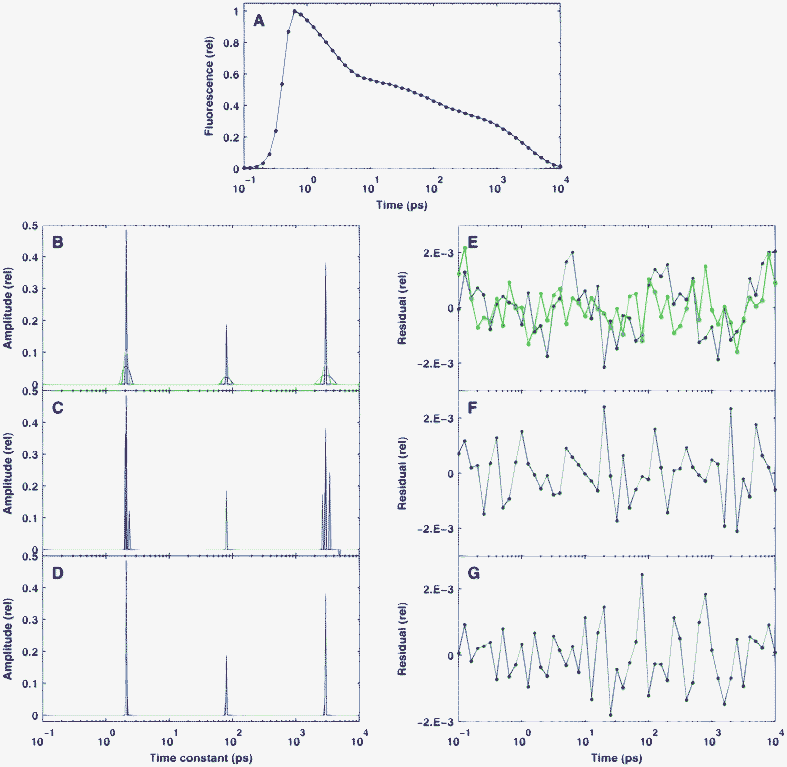

Fig. 1 Performance of different algorithms in the reconstruction of sparse, simulated fluorescence kinetics data. The true distribution is indicated by red lines. Panel A: the simulated fluorescence signal in time domain. Panels B–D: the recovered distribution calculated by GPSR (B blue line) , SpaRSA or TwIST (B green line), SparseBayes (C), L1-homotopy, l1-ls or SparseLab (D). Panels E–G: the residuals corresponding to (B–C). The standard deviation of the Gaussian noise which added to the simulated time-domain data was δ = 10⁻³. The regularization parameter used for the BPDN algorithms (B and D) was λ = 3 × 10⁻⁴.

It was found that BDPN routines in the GPSR, SpaRSA and TwIST toolboxes converged very badly for our problem. Stopping the optimization after 10⁵ iterations, the reconstruction of the original model by these programs resulted in relatively wide peaks, although at the correct places (Fig. 1B). In contrast to this, the reconstructed distribution calculated by SparseBayes (Fig. 1C) is much sparser, but contains extra peaks close to the real ones. This means that while the underlying Bayesian approach is very promising, this parameter-free procedure is not yet matured enough for the analysis of fluorescence kinetics. All of the l1-ls, SparseLab and L1-homotopy toolboxes reconstructed the true model excellently (Fig. 1D), although they are based on different optimization algorithms. The reconstructed peaks typically consist of only two points with non-negligible amplitude. However, we found differences in the speed of these toolboxes, as l1-ls solved our test ∼100 times slower than SparseLab and L1-homotopy, which behaved equally well under this test in every context. The latter routines performed excellently: with an experimental matrix of typical size (51 × 412), the optimization was executed in ∼150 ms on a medium category personal computer. The execution time was found to depend linearly on both dimensions of the matrix. All of the further calculations were carried out by SparseLab.

The residuals of the fitting presented in Fig. 1E–G are very similar to each other and do not show any structure. This fact, together with the lack of extra peaks in the solution indicates that the chosen value of λ = 3 × 10⁻⁴ ensures a good balance between good quality fit and highly regularized solution. Unless otherwise stated, this value of the regularization parameter was not changed during the forthcoming calculations. On the other hand, the similarity of the residuals corresponding to highly sparse and less sparse solutions underlines the ill-posed nature of the problem.

3.2 Simulation results with sparse kinetics

One of the main advantages expected from the sparse analysis of fluorescence kinetics is a good resolution for closely located peaks. To test this ability of the BPDN procedure, we calculated the reconstruction of a true distribution identical to that studied in the previous section, but containing an additional peak separated by only 8 channels from the neighbouring one. This separation is equivalent to a ratio of ∼1.37 for the corresponding time constants. Clearly, in the presence of simulated noise, the pattern of a reconstruction depends not only on its level but also its random actualization. Accordingly, the reconstruction patterns shown in Fig. 2 represent only typical patterns, corresponding to different noise levels. The selected three values (10⁻², 10⁻³ and 10⁻⁴) for the standard deviation of noise on the top of a normalized signal correspond to a poor, a reasonable, and a very high quality real measurement, respectively. (Assuming Poisson statistics for the photon noise—which is approximated here by Gaussian distribution—these noise levels could be realized at 10⁴, 10⁶ and 10⁸ peak photon counts, respectively.)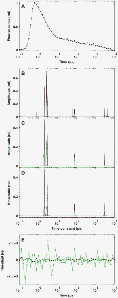

Fig. 2 Reconstruction of sparse simulated kinetics defined by positive amplitudes in the presence of different levels of Gaussian noise on the time-domain data. The true distribution is indicated by solid red lines. Panel A: the simulated signal in time domain with a noise level of δ = 10⁻² (red dots) and its fitting curve (solid black). Panels B–D: the reconstructed distributions at noise levels of δ = 10⁻² (B), δ = 10⁻³ (C) and δ = 10⁻⁴ (D). Panel E: the residuals corresponding to C (green) and D (blue).

At a noise level of δ = 10⁻² (Fig. 2A–B), the solution consists of four major peaks, the positions of which, in some cases, are considerably biased from the true one. The bias is typically downward for low τ values and upward for high ones. In addition, the appearance of small extra peaks (both positive and negative) is also observable. Both effects are a consequence of the balance between good fit and high sparsity at the given level of noise and regularization parameter: the constraint for good fit results in extra peaks, while that for high sparsity causes bias in the solution. As one expects, at δ = 10⁻³ the bias is highly reduced and the amplitudes of the non-valid peaks become negligible, and this tendency further increases at δ = 10⁻⁴. Importantly, the clear separation of the two closely located peaks took place in the majority of our tests at any noise level.

Since the solution patterns show such high dependency on noise, beyond the above typical examples it is also informative to calculate the average of solutions obtained with the same level but a different realization of random noise. Therefore, we calculated the average of 100 solutions corresponding to the same true model presented in Fig. 2, but different actual sets of random noise added to the simulated time-domain kinetics. The results are shown in Fig. 3, where the averages depicted in panels A–C correspond to the individual solutions presented in Fig. 2B–D, respectively. At a noise level of δ = 10⁻² (Fig. 3A) the positions of the two peaks in the region of high time constants are very uncertain, as is manifested in the appearance of broad bands of small amplitudes in the reconstruction, while the two closely located true peaks around 2 and 3 ps are represented by a unimodal, moderately wide band between them. As expected, the peak localization noticably increases with a decreasing level of noise, but the two close peaks are resolved in the reconstruction only at δ = 10⁻⁴ (Fig. 3C). Another way to increase the resolution in the averaged distributions is to increase the density of sampling in the time-domain kinetics, as presented in panel D of Fig. 3, where the noise level is identical to that in panel B but the time-domain sampling is 4-fold that of the usual one. Comparing Fig. 2 and 3, one can conclude that the individual and the averaged solutions hold somewhat complementary information: an individual solution is always sparser, and hence provides better resolution, while the averages inform us about the uncertainty of the peak position corresponding to a certain level of noise, with the expense of reduced resolution.

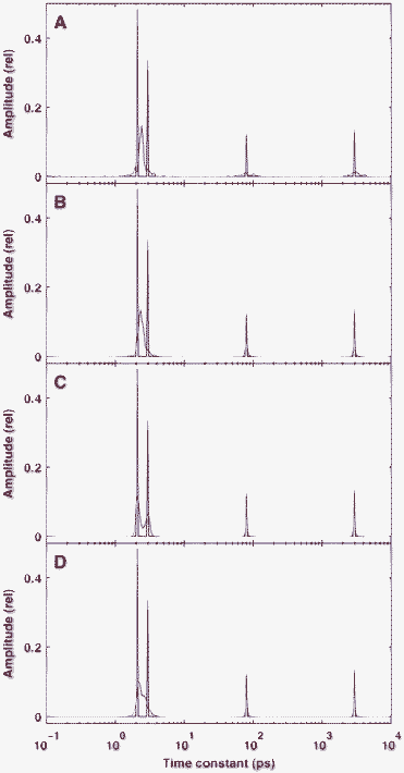Fig. 3 Average of 100 reconstructed distributions calculated from the same true model but different noise data added to the time-domain kinetics. The true distribution is identical to that presented in Fig. 2 and indicated by red lines. The levels of Gaussian noise were δ = 10⁻² (A), δ = 10⁻³ (B and D) and δ = 10⁻⁴ (C). In panel D the reconstruction was based on simulated kinetics calculated at 40 time points in a decade instead of the usual 10.

In our final example on the reconstruction of sparse kinetics we also included a negative peak in the true distribution. The BPDN procedure naturally includes this possibility, although in the l1-ls implementation, a positivity constraint is also allowed. The true distribution in this simulation was similar to that found in the analysis of real fluorescence kinetic measurements carried out in FAD (see Section 3.4). As a consequence of the well-separated non-zero values in this distribution, at a medium noise level of δ = 10⁻³, the reconstruction of the positive peaks in a single simulation (Fig. 4A) was excellent, and the average of 100 calculations (Fig. 4B) was hardly different from that. On the other hand, the location of the negative peak at the low end of the distribution showed some bias in both the individual and the averaged solutions. This level of noise allowed the reduction of the regularization parameter by a factor of ten without a considerable decrease of sparsity in the solution (Fig. 4C). This reduction increased the goodness of fit, manifested as the disappearance of bias in the position of the negative peak.

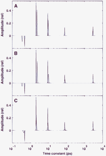Fig. 4 Reconstruction of a sparse distribution containing both positive and negative peaks. The true distribution is indicated by red lines. The noise level on the simulated time-domain data was δ = 10⁻³. Panel A: reconstruction from a single simulation with regularization parameter of λ = 3 × 10⁻⁴. Panels B and C: average of 100 reconstructions with λ = 3 × 10⁻⁴ (B) and λ = 3 × 10⁻⁵ (C).

3.3 Simulation results with distributed kinetics

As shown in the previous section, the BPDN procedure performed rather well in the reconstruction of sparse kinetics: the solutions remained sparse even in the presence of noise, and the resolution as well as the precision of the peak positions increased as the level was reduced. A naturally arising question is how does this procedure behave if the underlying true distribution is not sparse? The ill-posed nature of the problem dictates that this approach could easily find a sparse solution which approximates distributed kinetics well. To investigate this interesting problem we carried out simulations with true distributions which were highly dense. In our test, presented in Fig. 5, the true distribution on the logarithmic space of time constants was made up of two Gaussians with FWHMs of 50 and 20 (see red curves in panels A–C).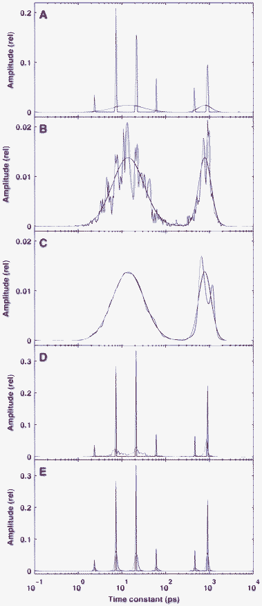

Fig. 5 Performance of the sparse analysis in the reconstruction of distributed kinetics. The true distributions are indicated by red lines. Panel A: reconstruction from a single simulation with a noise level of δ = 10⁻³ and a regularization parameter of λ = 3 × 10⁻⁴. Panel B: average of 100 reconstructions with δ = 10⁻³ and λ = 3 × 10⁻⁴. Panel C: average of 100 reconstructions with δ = 10⁻⁴ and λ = 3 × 10⁻⁵. Panels D and E: average of 100 reconstructions from a sparse true distribution, similar to the result of the reconstruction presented in panel A with λ = 3 × 10⁻⁴, δ = 10⁻³ (D) and δ = 10⁻⁴ (E).

Indeed, with the usual noise level of δ = 10⁻³ and regularization parameter of λ = 3 × 10⁻⁴, the typical individual reconstruction was sparse, and the two Gaussians were approximated by four and two narrow peaks, respectively (Fig. 5A). Interestingly, however, under these circumstances the positions of these peaks were very uncertain and the average of 100 solutions (Fig. 5B) clearly indicated the distributed nature of the kinetics and followed the shape of the true distribution. We have also found that in this context, averaging the solutions corresponding to different realizations of noise is more informative than averaging the data first and calculating the solution after that. In the latter case the solution consists of broadened peaks (data not shown) but still much more sparse than in the former one. Under very good conditions for high quality fitting (δ = 10⁻⁴ and λ = 3 × 10⁻⁵) the reconstruction with the averaged solutions was almost perfect even in the case of this very unfavoured problem for the BPDN procedure (Fig. 5C).

Since a sparse but invalid solution such as the one presented in Fig. 5A can fit the time-domain kinetics very well, we also tested the ability of the applied procedure to distinguish between truly sparse and distributed kinetics if their time-domain shapes are very similar. To that end, we carried out simulations also with a sparse true distribution having a similar shape to the one that occurred as a sparse solution of the distributed kinetics (red curves in Fig. 5D–E). It was found that even if the noise level is δ = 10⁻³, the sparse or non-sparse nature of the underlying true distribution is clearly distinguishable from the reconstruction (compare panels B and D in Fig. 5) and becomes even more clear if the noise is reduced further (Fig. 5E).

The above results point out again that a sparse (or any other kind of) analysis of a single kinetics cannot provide reliable information on the nature of the underlying kinetics. Throughout our simulations, additional useful information was obtained from the average of solutions corresponding to different realizations of noise. Of course, in real practice with experimental data, this approach would be very time-consuming. Fortunately, similar information can be gained if the measurements are not simply repeated but an extra relevant parameter (like wavelength) is varied, as discussed in the next section.

Clearly, if it is known a priori that the kinetics are distributed, the BPDN method is not the ideal way for a final analysis. In that case MEM, which favours minimum structure in the solution,¹¹ could be a more adequate method or a kind of model-based analysis^19–21 is even better if that is possible. However, such a priori knowledge rarely exists, especially for new types of studies. In that case, a BPDN analysis is always a good starting point, which—if the results so indicate—can be extended by other methods performing less effectively for sparse kinetics. The direct comparison of BPDN and MEM on the same dataset of different degrees of sparsity is beyond the scope of the present study, although such an analysis carried out in the future would be very interesting.

3.4 Analysis of real experimental data

For testing the capabilities of the BPDN method on real experimental data, we applied this method for the analysis of a fluorescence kinetic dataset measured on the aqueous solution of FAD. The time- and wavelength-dependent fluorescence data obtained by a combined method of fluorescence up-conversion and TCSPC (see Section 2.1) is presented in Fig. 6 by blue lines. The BPDN analysis was carried out independently at every wavelength. The signal/noise ratio of the data was inherently higher in the section measured by TCSPC, which was increased even more by the logarithmic compression. The average value of the normalized noise level at the wavelength of the maximum (530 nm) was around δ = 5 × 10⁻³, and accordingly the regularization parameter was set to λ = 3 × 10⁻⁴, as usually done in the course of simulations. The fit obtained by this value with the experimental data is presented by the red curves in Fig. 6.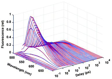

Fig. 6 Time and wavelength dependence of the fluorescence from 1.5 × 10⁻³ M FAD in water (pH = 8.0). Blue lines: experimental data, red lines: fitting by BPDN with λ = 3 × 10⁻⁴.

As stated above, the typical solution corresponding to a single wavelength is similar to that shown by the red line in Fig. 4; it consists of five narrow peaks located at around 500 fs, 2 ps, 10 ps, 80 ps and 3 ns. The distribution of the amplitudes on the 2D space of time constants and wavelengths is presented in Fig. 7, where zero, positive and negative amplitudes are coloured green, red and blue, respectively. Remarkably, the overall distribution looks very sparse, albeit the range of the amplitudes mapped to the colour scale was set to very narrow in the figure. In addition, the significant non-zero amplitudes are distributed in almost straight strips along the wavelength scale, despite the lack of any constraint in the analysis favouring wavelength independence of the dominating time constants. Some deviations from this arrangement take place only at low wavelengths where the signal/noise ratio is poor. This distribution clearly indicates that the kinetics are truly sparse, otherwise the strips would be more diffuse and less separated due to the high uncertainty in the locations of the peaks, as discussed in the previous section. In this context, the BPDN analysis of experimental data taken by varying the wavelength (or any other independent parameter), provides useful information about the level of sparsity of the underlying kinetics, similarly to that obtained by simple averaging of the solutions as done in the previous simulations.

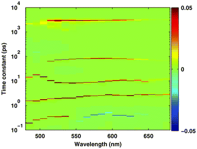Fig. 7 Distribution of the amplitudes on the space of time constants and wavelengths in the result of BPDN analysis of FAD fluorescence kinetics presented in Fig. 6.

The appearance of the well-separated narrow strips in the solution entitles us to represent their traces by simple lines as shown in Fig. 8A. A point of such a line at a given wavelength was calculated as the statistical mean of the time constants using the amplitudes corresponding to each significant peak as weighting factors. The sum of these amplitudes plotted against the wavelengths is presented in Fig. 8B. This plot corresponds to the decay-associated spectra (DAS), a concept frequently used in traditional analysis.^7,44

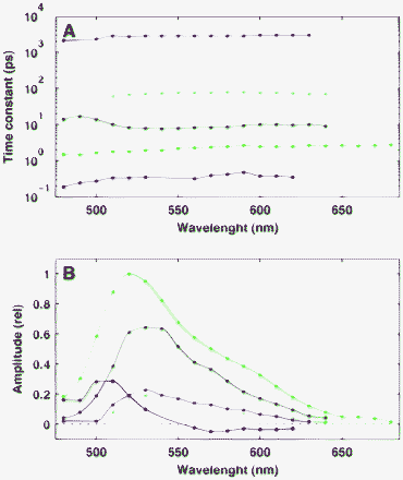Fig. 8 Panel A: Traces of the statistical mean of the time constants corresponding to the different strips in Fig. 7. Panel B: Decay-associated spectra of each component in panel A.

The result of the sparse analysis summarized in Fig. 8 can be interpreted by the existence of five independent, exponentially decaying components in the fluorescence kinetics of FAD. The DAS of the fastest component (red lines in Fig. 8) shows a special structure: it is positive at the low spectral region but negative above 560 nm. Such a typical structure suggests that the underlying process is probably related to the solvation dynamics of water molecules around the fluorescent chromophore.³¹ This interpretation is in good agreement with the ∼500 fs lifetime of the component which is close to the reported 800 fs solvation response time which is characteristic of the diffusion motion in bulk water.⁴⁵ A decaying component of ∼800 fs lifetime and a blue-shifted spectrum was also attributed to solvation dynamics in a previous study.⁴⁶

It is far beyond the scope of this paper to assign the other four decaying components to particular chemical structures of the FAD molecules. Notably, the DASs corresponding to these components are very similar to each other as well as to the static emission spectrum of FAD in water.⁴⁷ Previous time-resolved fluorescence studies agreed on the model according to which FAD molecules in water solution can exist both in open and stacked conformations. The nanosecond components of the fluorescence decay were assigned to the former while the subnanosecond ones to the latter type of conformations.^46–48 However, the number and the values of the observed time constants reported in the literature are still ambiguous, mainly due to the fragmented time intervals in which the measurements were carried out. A systematic study on this problem, with the methods presented in this paper, is in progress in our laboratory.

4 Conclusions

We have found that the novel concept of compressed sensing can be successfully applied both in the acquisition and the analysis of time-resolved fluorescence data. On the experimental side, the data obtained by the method of fluorescence up-conversion and TCSPC in a single setup were combined into a common dataset on a logarithmic timebase. The main advantage of this approach is that a large number of different kinetic components, spanning a wide range in their time constants, can be represented in the experimental data with equal weights. At the same time the acquired dataset is kept compressed as the number of required data points is very low.

On the side of analysis, we have shown that the application of the BPDN procedure results in a highly compressed solution: although many parameters are allowed to contribute in the modelling of the data, only a few of them are found to actually do so. Our simulations indicated that if the underlying kinetics are truly sparse, their parameters are excellently recovered by this approach. It was found that the single solutions of the BPDN analysis and the average of them in the presence of a different actualization of noise provide complementary information: the former has a superior resolution while the latter yields the probability distribution of the location of the contributing time constants. Such a distribution provides valid information even if the true kinetics are far from sparsity. Finally, a case study with real experimental data indicated that complex yet still sparse information can be obtained from the fluorescence kinetics if an additional independent parameter, such as wavelength, is also varied.

The above results indicate that the application of the BPDN procedure (which has a negligible time cost over that of the data acquisition) is a powerful and novel method for the analysis of time-resolved fluorescence data. In comparison to the traditional methods it is worth noting that, like MEM, this method represents a model-free approach, and that like every method based on a regularization technique described by (4), this kind of analysis does not provide any unique value characterizing the goodness of fit. Instead of using such a single number for evaluation, the best practical strategy for gaining the most complete information on the nature of the underlying kinetics (e.g. for distinguishing between truly sparse and distributed kinetics) is to repeat the measurement by varying the wavelength or any other additional parameter. If the obtained distribution (illustrated in Fig. 7) is still not satisfactory in its resolution or peak localization, one needs to improve the quality of the measurement by increasing the sampling density and the signal/noise ratio.

Acknowledgements

This work was supported by the National Development Agency of Hungary (grants TÁMOP-4.2.2-08/1-2008-0001, TECH-09-A2-2009-0134 and TÁMOP-4.2.1/B-09/1/KONV-2010-0005) and co-financed by the European Regional Fund.

References

1. J. R. Lakowicz, Principles of fluorescence spectroscopy, 3^rd edn, Springer, New York, 2006.
2. D. Chorvat and A. Chorvatova, Laser Phys. Lett., 2009, 6, 175–193.
3. G. Landl, T. Langthaler, H. W. Engl and H. F. Kauffmann, J. Comput. Phys., 1991, 95, 1–28.
4. J. T. Giurleo and D. S. Talaga, J. Chem. Phys., 2008, 128, 114114.
5. A. Siemiarczuk, B. D. Wagner and W. R. Ware, J. Phys. Chem., 1990, 94, 1661–1666.
6. J. R. Knutson, J. M. Beechem and L. Brand, Chem. Phys. Lett., 1983, 102, 501–507.
7. I. H. M. van Stokkum, D. S. Larsen and R. van Grondelle, Biochim. Biophys. Acta, Bioenerg., 2004, 1658, 262–262.
8. J. J. Fisz, J. Phys. Chem. A, 2006, 110, 12977–12985.
9. Y. S. Liu and W. R. Ware, J. Phys. Chem., 1993, 97, 5980–5986.
10. A. K. Livesey and J. C. Brochon, Biophys. J., 1987, 52, 693–706.
11. J. C. Brochon, Methods Enzymol., 1994, 240, 262–311.
12. R. Swaminathan and N. Periasamy, Proc. Indian Acad. Sci.-Chem. Sci., 1996, 108, 39–49.
13. V. A. Lorenz-Fonfria and H. Kandori, Appl. Spectrosc., 2007, 61, 74–84.
14. A. Visser, S. P. Laptenok, N. V. Visser, A. van Hoek, D. J. S. Birch, J. C. Brochon and J. W. Borst, Eur. Biophys. J., 2010, 39, 241–253.
15. S. Haldar, M. Kombrabail, G. Krishnamoorthy and A. Chattopadhyay, J. Fluoresc., 2010, 20, 407–413.
16. E. T. Jaynes, in Papers on Probability, Statistics an Statistical Physics, ed. R. D. Rosenkrantz, Kluwer, Dordrecht, 1983, pp. 210–314.
17. J. Skilling, in Maximum Entropy and Bayesian Methods, Cambridge, England, 1988, ed. J. Skilling, Kluver, Dordrecht, 1989, pp. 45–52.
18. S. F. Gull, in Maximum Entropy and Bayesian Methods, Cambridge, England, 1988, ed. J. Skilling, Kluver, Dordrecht, 1989, pp. 53–71.
19. J. R. Alcala, E. Gratton and F. G. Prendergast, Biophys. J., 1987, 51, 597–604.
20. J. R. Alcala, E. Gratton and F. G. Prendergast, Biophys. J., 1987, 51, 925–936.
21. A. C. Fogarty, A. C. Jones and P. J. Camp, Phys. Chem. Chem. Phys., 2011, 13, 3819–3830.
22. M. N. Berberan-Santos, E. N. Bodunov and B. Valeur, Chem. Phys., 2005, 315, 171–182.
23. M. N. Berberan-Santos, E. N. Bodunov and B. Valeur, Chem. Phys., 2005, 317, 57–62.
24. V. Souchon, I. Leray, M. N. Berberan-Santos and B. Valeur, Dalton Trans., 2009, 3988–3992.
25. M. E. Tipping, in Advanced Lectures on Machine Learning, ed. O. Bousquet, U. von Luxburg and G. Rätsch, Springer, 2004, pp. 41–62.
26. E. J. Candes and M. B. Wakin, IEEE Signal Process. Mag., 2008, 25, 21–30.
27. D. L. Donoho, M. Elad and V. N. Temlyakov, IEEE Trans. Inf. Theory, 2006, 52, 6–18.
28. D. L. Donoho, Commun. Pure Appl. Math., 2006, 59, 907–934.
29. S. S. B. Chen, D. L. Donoho and M. A. Saunders, SIAM J. Sci. Comput., 1998, 20, 33–61.
30. M. E. Tipping and A. C. Faul, in Proceedings of the Ninth International Workshop on Artificial Intelligence and Statistics, Jan 3-6, 2003, Key West, FL., ed. C. M. Bishop and B. J. Frey, Society for Artificial Intelligence and Statistics, 2003.
31. D. P. Zhong, S. K. Pal, D. Q. Zhang, S. I. Chan and A. H. Zewail, Proc. Natl. Acad. Sci. U. S. A., 2002, 99, 13–18.
32. SparseLab toolbox, http://sparselab.stanford.edu..
33. L1 Homotopy toolbox, http://users.ece.gatech.edu/.
34. M. S. Asif and J. Romberg, IEEE J. Sel. Topics Signal Process., 2010, 4, 421–434.
35. l1_ls toolbox, http://www.stanford.edu/.
36. S. J. Kim, K. Koh, M. Lustig, S. Boyd and D. Gorinevsky, IEEE J. Sel. Top. Signal Process., 2007, 1, 606–617.
37. GPSR toolbox, http://www.lx.it.pt/.
38. M. A. T. Figueiredo, R. D. Nowak and S. J. Wright, IEEE J. Sel. Top. Signal Process., 2007, 1, 586–597.
39. SpaRSA toolbox, http://www.lx.it.pt/.
40. S. J. Wright, R. D. Nowak and M. A. T. Figueiredo, IEEE Trans. Signal Process., 2009, 57, 2479–2493.
41. TwIST toolbox, http://www.lx.it.pt/.
42. J. M. Bioucas-Dias and M. A. T. Figueiredo, IEEE Trans. Image Process., 2007, 16, 2992–3004.
43. SparseBayes toolbox, http://www.relevancevector.com..
44. J. R. Knutson, D. G. Walbridge and L. Brand, Biochemistry, 1982, 21, 4671–4679.
45. R. Jimenez, G. R. Fleming, P. V. Kumar and M. Maroncelli, Nature, 1994, 369, 471–473.
46. H. Chosrowjan, S. Taniguchi, N. Mataga, F. Tanaka and A. J. W. G. Visser, Chem. Phys. Lett., 2003, 378, 354–358.
47. T. Nakabayashi, M. S. Islam and N. Ohta, J. Phys. Chem. B, 2010, 114, 15254–15260.
48. P. A. W. van den Berg, K. A. Feenstra, A. E. Mark, H. J. C. Berendsen and A. J. W. G. Visser, J. Phys. Chem. B, 2002, 106, 8858–8869.

---