Predictive methods for the estimation of thermophysical properties of ionic liquids
João A. P.
Coutinho
*a,
Pedro J.
Carvalho
a and
Nuno M. C.
Oliveira
b
aDepartamento de Química, CICECO, Universidade de Aveiro, 3810-193, Aveiro, Portugal. E-mail: jcoutinho@ua.pt; quijorge@ua.pt; Fax: +351 234 370 084; Tel: +351 234 401 507
bDepartamento de Engenharia Química, Faculdade de Ciências e Tecnologia, Universidade de Coimbra, Rua Sílvio Lima - Pólo II. 3030-790, Coimbra, Portugal. E-mail: nuno@eq.uc.pt; Fax: +351 239 798 703; Tel: +351 239 798700
First published on 18th April 2012
Abstract
While the design of products and processes involving ionic liquids (ILs) requires knowledge of the thermophysical properties for these compounds, the massive number of possible distinct ILs precludes their detailed experimental characterization. To overcome this limitation, chemists and engineers must rely on predictive models that are able to generate reliable values for these properties, from the knowledge of the structure of the IL. A large body of literature was developed in the last decade for this purpose, aiming at developing predictive models for thermophysical and transport properties of ILs. A critical review of those models is reported here. The modelling approaches are discussed and suggestions relative to the current best methodologies for the prediction of each property are presented. Since most of the these works date from the last 5 years, this field can still be considered to be in its infancy. Consequently, this work also aims at highlighting major gaps in both existing data and modelling approaches, identifying unbeaten tracks and promising paths for further development in this area.
1. Introduction
The academic and industrial interest in ionic liquids (ILs) is well established today. The former is clear from the exponential number of publications on this subject, with more than 8000 articles published during 2011 alone, making this field one of the fastest growing areas in chemistry. The industrial importance of ILs is reflected by the number of commercial processes and products based on these compounds currently in the market.1–7 The design of these products and processes requires knowledge of the thermophysical and transport properties of ILs. However, given the vast number of potential candidates, the experimental characterization of all of these fluids is unfeasible. Seddon2,8,9 has been variably establishing their number from 106![[thin space (1/6-em)]](https://www.rsc.org/images/entities/char_2009.gif) 2,8 to 1018,9 but even in the lower limit of this interval the selection of ILs for practical purposes is a task that cannot be carried out by trial and error easily.
2,8 to 1018,9 but even in the lower limit of this interval the selection of ILs for practical purposes is a task that cannot be carried out by trial and error easily.
To circumvent this daunting mission and help chemists and engineers selecting ILs and designing their products and processes, predictive models and correlations for the thermophysical and transport properties of ILs have been proposed by a growing number of researchers. Encumbered at first by the limited amount of available data and its off-putting quality, the growing body of data and the accessibility of some reliable databases10 is making the task of modellers easier, and their models more widely applicable, sound and reliable. Yet, if for some properties data is now available for more than 1000 ILs,11 as is the case for density, other properties seems to lag behind, such as speed of sound, refractive index or transport properties such as diffusion and self-diffusion coefficients or thermal conductivities. The development of equations of state (EoS) for the description of ILs could be fostered by the availability of reliable speeds of sound, given the impossibility of measuring critical properties or vapour pressures commonly used for this purpose. The importance of transport properties in the industrial application of ILs does not need to be stressed here. It is enough to say that one of the more innovative applications of ILs as a liquid piston in the hydrogen compressors developed by Linde2,7 relies on their ability to dissipate the heat generated during compression, and that there is a growing interest in their application as heat transfer fluids. However, the open literature has little more than a dozen data points for a handful of ILs, and little progress has been observed on this subject in the last few years. An extra effort is therefore required from experimentalists to produce enough reliable data for new models to be developed and tested. Two recent reviews on the thermophysical properties of ILs are available for the interested reader.12,13
Many different approaches to the development of predictive models for thermophysical and transport properties of ILs have been proposed. These are grouped in Fig. 1, according to the methodology used for their development. The equations of state have a theoretical basis that generally makes them good candidates for the prediction of thermophysical properties such as density, vapour pressure, enthalpy of vaporization, surface tension, speed of sound and heat capacity. Although EoS have been used with ILs by a number of authors, their wider application is currently encumbered by the lack of feasible approaches for estimating the required model parameters. In practice, this constrains their role to tasks closer to experimental data correlation. Albeit useful, this approach is considered outside of the scope of this review; nevertheless, a recent review on the use of equations of state for the description of IL systems is available.14 We also chose not to cover the use of molecular simulation techniques in this review. Despite the success that they have known in the description of the thermophysical and phase equilibrium properties of ILs15,16 (this success is more mitigated for the transport properties), the estimation of properties based on molecular simulation techniques remains a complex and lengthy task that, despite its undeniable interest, is not yet an ordinary tool for the engineer in the design of new processes and products. Nevertheless, we have included in this review both QSPR (quantitative structure activity relationship) approaches and other correlations that are based on information retrieved from molecular simulation calculations, since these data can be kept in accessible databases (e.g., the COSMO-RS based information used by several correlations). Also outside the scope of this review are the mixture and equilibrium properties of ILs with other compounds, which are also fundamentally important for chemical process and product development.
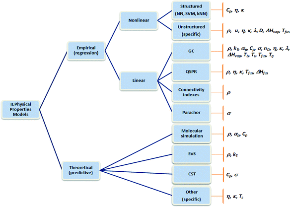 | ||
| Fig. 1 Classes of methodologies used in the determination of the thermophysical properties of ILs. | ||
The possibility of tailoring the properties of an IL to meet the requirements of a specific application seems to be one of their most promising characteristics. Given the huge number of potential ILs, the use of empirical heuristics for their selection17 might be useful. However, this approach can be difficult to generalize for more specific demands, and unable to provide answers of sufficient quality when a best match is sought. In a significant number of cases, fulfilling the potential provided by the large number of molecular combinations requires the use of systematic methodologies, such as the ones provided by the area of Computer Aided Molecular Design (CAMD).18,19 These techniques typically allow the solution of an inverse problem: given a set of specifications or property constraints, they work backwards to identify and rank the subsets of molecules that satisfy these particular criteria. To be more effective than a simple database look-up, CAMD methodologies require the availability of quantitative models for ILs that relate the values of the physical properties to their molecular structure. This allows the use of algorithms for numerical optimization and logical constraint satisfaction problems, where a large solution space can be implicitly enumerated very efficiently, to provide optimal solutions.20,21 The successful integration of models of physical properties in CAMD nevertheless imposes specific requirements on the structure of these models, namely:
•The properties should be computable for arbitrary (e.g., previously unseen) molecules, based solely on the knowledge of their structure.
•The computation should be based on easily accessible descriptors, and be feasible for general purpose computational environments.
•The models need to be able to be used reversibly, e.g., from structure to properties and from properties to feasible structures.
•The methods should also provide a characterization of the uncertainty of their predictions, required for effective constraint satisfaction and solution ranking.
All of these additional requisites need to be taken into account in the development phase of thermodynamic models due to the ever more widespread use of CAMD methodologies in the design of chemical processes and products. A practical consequence of the above requirements is that, despite their empirical nature, the classes of methods derived through regression (Fig. 1) currently seem to be more popular with ILs, with particular emphasis on group contribution (GC) models. Quantitative structure–activity relationships (QSPR) and correlations with other properties (e.g., the Stokes–Einstein law for the diffusion coefficients, the Walden rule for conductivities, or the Auerbach relation for sound velocities) follow closely. As described below, connectivity indexes (CI) have also recently received some recognition, but their applications are still more limited.
As well as linear contribution methods, nonlinear regression procedures are also attractive for the development of thermophysical properties models, due to their increased flexibility, often leading to more parsimonious models. In the group of structured approaches to nonlinear regression, neural networks22–24 (NN) have been tested and have had some success in the prediction of the properties of ILs in recent years. Additional techniques in this group of machine learning algorithms, such as support vector machines (SVM) and k-nearest neighbours (kNN),25 have also been used with ILs. These are reviewed here to make their applications better known, since the lack of familiarity of the developers with these types of modelling approaches has clearly hampered their application in the past. Similarly to other classes of models, not all members of this family satisfy the previous constraints relative to the integration of these property models in CAMD approaches; for instance, typical NN structures can only be used in forward (prediction) mode. Still, as in other application areas, the development of these models can be extremely useful for the exploratory discovery of interesting relationships between physical properties, and this analysis can be later complemented by additional investigation using alternative modelling approaches.
This review is structured along the conventional division of thermophysical, transport and equilibrium properties. For each property a detailed list of the predictive methods available along with their reported accuracy is presented. The final section comprises a critical discussion on the merits and limitations of the approaches used. Suggestions relative to the best models currently available for each property studied here are also given.
2. Volumetric properties
2.1 Density
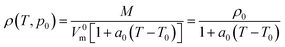
The density (ρ) is one of the most studied properties of ILs, with about 20000 data points currently available for more than 1000 ILs in temperature and pressure ranges of 253–473 K and 0.1–300 MPa, respectively.11 Given the availability of data and the relevance of this variable, it is not surprising that this, along with the melting temperatures, is the property for which most correlations and models have been proposed for its estimation.
After a preliminary attempt by Trohalaki et al.,26 using a QSPR correlation valid only for 1-substituted 4-amino-1,2,4-triazolium bromides, the first correlation of general application was proposed by Ye and Shreeve.27 Their model is based on the group additivity concept and uses the hypothesis of Jenkins28 that the molar volume of the salt (Vm) is the linear sum of the cation and anion molar volumes. Therefore, for an MpXq salt
| Vm = pV+m + qV−m | (1) |
where Vm, Vm+, and Vm− are the molar volumes of the IL, cation and anion respectively, and the density is estimated by
 | (2) |
where MW is the IL molecular weight.
Using the ion molar volumes taken from Jenkins' work28 and the volume parameters for other functional groups as reported in the literature or refined from existing density data, Ye and Shreeve27 proposed a parameter table of about 60 parameters covering 12 cation families and 20 anions. Using their model, they reported that 40.6% of the estimated densities were within an absolute deviation of 0.0–0.02 g cm−3, 29.3% were within 0.021–0.04 g cm−3, 16.6% were within 0.041–0.06 g cm−3, 8.8% were within 0.061–0.08 g cm−3, and less than 5% were above this value. Although this approach produced good predictions for the densities of ILs, its major limitation is that it is only valid at 298.15 K and 0.1 MPa.
Curiously, a similar idea was simultaneously proposed by Slattery et al.29 but it was much less developed, and no attempt at refining the parameters estimated from the crystal structures was made, leading to much larger deviations and a very limited parameter table was reported. The deviations for the densities of 21 ILs are of the order of 1.8%.30
Aiming at extending Ye and Shreeve's27 approach to a wider range of pressure and temperature conditions, Gardas and Coutinho31 proposed an extension of this model, which assumed that the mechanical coefficients of the ILs, the isothermal compressibility (κT) and the isobaric expansivity (αP) are constant in a wide range of pressures (p in MPa) and temperatures (T in K), and similar for all ILs. This lead to the following molar volume dependency on pressure and temperature for Ye and Shreeve's27 molar volume (V0):
| Vm = V0(A + BT + Cp) | (3) |
From here the densities could be calculated as:
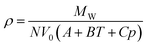 | (4) |
The values of the coefficients A, B and C, estimated by fitting eqn (4) to about 800 experimental data points, are 8.005 × 10⁻¹ ± 2.333 × 10⁻⁴, 6.652 × 10⁻⁴ ± 6.907 × 10⁻⁷ K−1 and −5.919 × 10⁻⁴ ± 2.410 × 10⁻⁶ MPa−1, respectively, at the 95% level of confidence. Gardas and Coutinho further extended the parameter table for previously unavailable cations. The extended version of the Ye and Shreeve model27 can predict densities of ILs in a wide range of temperatures 273.15–393.15 K and pressures 0.10–100 MPa. For imidazolium-based ILs, the average deviation reported was 0.45%, for phosphonium 1.49%, 0.41% for pyridinium and 1.57% for pyrrolidinium-based ILs. The model also provides a good representation of the densities of binary mixtures of ILs having a common cation or anion. Extensions of the parameter table for other ions have been reported.32–37 Recently, Aguirre and Cisternas38 have shown it to be applicable to ammonium based ILs with a 1.57% deviation.
Another model based on the additivity concept of Jenkins28 was proposed by Jacquemin et al.39 Instead of using a group contribution approach, they proposed a large temperature dependent parameter table for 44 anions and 104 cations, from which the ion molar volumes may be estimated using:
 | (5) |
Here δT = (T − 298.15 K) and Ci are the coefficients obtained by fitting the data at 0.1 MPa. The model is reported to produce an average deviation of less than 0.5% for a database of more than 2000 data points.
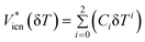
The major limitation of this approach is that it is only valid at 0.1 MPa. To eliminate this constraint, the authors proposed an extension of the model to high pressures.40 The revised model has 7 parameters to describe the temperature and pressure dependency of the molar volume of each ion, according to
 | (6) |
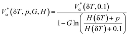
where α stands for the cation or anion, G is an adjustable parameter, V*α(δT, pref) is the reference effective molar volume obtained from the low pressure model and H(δT) is the second-order polynomial:
 | (7) |
H i parameters for 15 cations and 9 anions are reported by the authors. This model reproduces the IL molar volumes to within 0.36% using 5080 experimental data points (1550 and 3530 data points at 0.1 MPa and for p > 0.1 MPa, respectively).40 Although this model provides a good description of the experimental densities it is over parameterized and, with the exception of the alkyl imidazolium cations, it requires a set of 7 parameters for each ion. These characteristics make the fitting procedure and the use of the model somewhat cumbersome.
Qiao et al.41 proposed another group contribution model for the estimation of the densities of ILs. Unlike previous methods, the model does not estimate the molar volumes but calculates the density directly and uses both the Jenkins hypothesis of additivity applied to densities and the Gardas and Coutinho31 approach of constant mechanical coefficients as
| ρ = A + Bp + CT | (8) |
with p in MPa, T in K and where the parameters A, B and C are obtained by a group contribution method using a parameter table with 51 groups. The model was correlated to close to 7400 density data points for more than 120 ILs, and an average deviation of 0.88% for pure compounds and 1.22% for binary mixtures is reported.
Lazzús42 proposes a similar model that uses a group contribution approach to estimate the molar volumes of ILs (V0) at 298.15 K and 0.1 MPa, from which the corresponding density ρ0 = MW/V0 is calculated. This information is corrected to different temperatures and pressures by
| ρT,p = ρ0 + α(T − 298.15) + β(p − 0.101) | (9) |
where the constants of the model are α = 0.7190 and β = 0.5698. The group contribution parameter table is based on density data for 210 ILs and the pressure and temperature dependency has been regressed based on more than 3500 data points for 76 ILs. The model at the reference conditions (T0 = 298.15 K and p0 = 0.101 MPa) is reported to produce an average deviation of 1.9%, while the temperature and pressure dependent model has a deviation of 0.73%.
The most extensive group contribution model for ILs yet reported, based on approximately 20000 data points for more than 1000 ILs has been recently proposed by Paduszyński and Domanska.11 This is again a model for molar volumes based on Jenkins hypothesis of additivity of ion molar volumes28 and using the Gardas and Coutinho31 approach of constant mechanical coefficients and their identity for all ILs. The temperature dependency follows an approach previously used31
 | (10) |
but the authors adopt the Tait equation to obtain a better pressure dependency
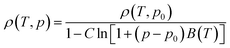 | (11) |
where:
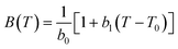 | (12) |
In eqn (10)–(12), the coefficients a0, C, b0 and b1 are adjustable parameters that are universal coefficients, i.e., they are the same for all ILs. Using this approach, unlike with that of Jacquemin et al.,40 the possibility of estimating the mechanical coefficients of the individual ILs is lost. However, the simplicity that it confers to the approach more than compensates for that loss, since a much lower number of parameters is required to describe the pρT behaviour of a wide number of ILs. The parameter table proposed is quite extensive, with 177 functional groups (including 44 cations and 70 anions), allowing for the estimation of the densities of a huge number of ILs. The authors report an average deviation of 0.53% for the 13000 points of the correlation set and of 0.45% for the 3700 point of the test set. A fair comparison reported by the authors of this model with other GC-models suggests this to be the best predictive model for densities yet reported.
Other approaches to the prediction of densities have been reported by several authors but they are either more complex or are of limited applicability, and in general provide predictions with larger deviations. Correlations with secondary properties such as molar refraction and parachor43 make little sense as these properties are known with far larger uncertainties, and are more difficult to measure than density. In one of the first works on the correlation of IL densities, Palomar et al.44 proposed a correlation between the experimental densities and molecular volumes and their corresponding predictions from COSMO-RS. This method is limited by the availability of the COSMO-RS database, and the correlations for the densities seem to be family dependent. If the density for a new molecule not present in the COSMO-RS database must be calculated the process becomes lengthy. The accuracy of the method is estimated to be better than 3%.44
The residual volume approach of Bogdanov and Kantlehner45 requires a correlation for each IL family, making it of limited applicability, while the correlation of density with the parachor proposed by Gardas et al.46 is meaningless since the parachor values are themselves estimated from a correlation with the molar volume. If the molar volume values are available then the correct and direct approach to density estimation is through eqn (3).
After the first efforts by Slattery et al.29 mentioned above, these authors proposed a new correlation between the densities47
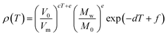 | (13) |
with c = 0.0001747 K−1, d = 0.0008028 K−1, V0 = 1 nm3, e =1.158, f = −7.413, M0 = 1 g mol−1 and V0 = 1 nm3. As in the model of Palomar et al.,44 the molar volumes (Vm) used in the correlation are estimated by a computational method (BP86/TZVP + COSMO). The authors claim that the method has comparable accuracy to Gardas and Coutinho,31 with deviations rarely exceeding 1%, though in some of the reported cases they can be as high as 3.6%. The method has not been extensively tested, with results reported only for a dozen ILs.
Besides the QSPR correlation of Trohalaki et al.,26 valid only for 1-substituted 4-amino-1,2,4-triazolium bromides, the only QSPR approach to the estimation of density was proposed by Lazzús.30 They reported the following correlation for the pressure and temperature dependency of the ILs densities, based on 7 descriptors for the cation and 4 for the anion:
| ρ(T,p) = −0.807(T − 298.15) + 0.410(p − 0.101) + 1.275(0.816[μc] + 15.972[IPc] − 1.793[LUMOc] − 0.104[Mc] − 0.375[Sc] + 0.034[Vc] + 107.235[σc])0.589 × (188.765[IPa] + 5.810[Ma] + 4.572[Sa] + 4.921[Va] + 1)0.408 | (14) |
The descriptors for the cation are molecular weight ([Mc]) in g mol−1, molecular surface area ([Sc]) in Å2, molecular volume ([Vc]) in Å3, ovality ([σc]), dipole moment ([μc]) in Debye, ionization potential ([IPc]) in eV and the lowest unoccupied molecular orbital energy ([LUMOc]) in eV. The descriptors for the anion are molecular weight ([Ma]), molecular surface area ([Sa]), molecular volume ([Va]), and the ionization potential ([IPa]), using the same units as in the cation case. These descriptors, derived from the PM3 Semi-Empirical Molecular Orbital Theory, were calculated by MOPAC-Chem3D. Average deviations of approximately 2% were obtained for the correlation and testing sets.
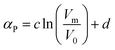
Connectivity indexes have recently had some popularity as a basis for the development of models for thermophysical properties. Two approaches based on this concept have been applied to the densities of ILs. Valderrama and Rojas48 proposed a mass connectivity index that allows the estimation of the temperature dependency of the density if the reference density ρ0 at a reference temperature T0 is known:
| ρ = ρ0 − 3.119 × 10⁻³λ(T − T0) | (15) |
Here, λ is the mass connectivity index, defined as the sum of the inverse of the mass connectivity interactions and calculated as the square root of the product of the mass of groups immediately connected in a molecule:
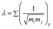 | (16) |
The authors used 479 data points for 106 ILs to determine the constant in eqn (15), while 50 values of density were predicted with an average deviation of 0.7% and a maximum deviation of 2.6%.
Xiong et al.49 proposed a volumetric connectivity index (σ) correlation that allows the estimation of the densities at 298.15 K as:
| ρ0 = aσ + b + c | (17) |
The constants a, b and c are fitted to experimental data, and their values reported for 51 groups by the authors. The volumetric connectivity index is defined as the sum of the inverse of the group volumetric connectivity interactions and is calculated as the square root of the product of the volumetric connectivity interaction parameters of the groups immediately connected in a molecule
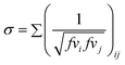 | (18) |
The authors report average deviations of 0.63% and maximum deviations of 4.0% for 142 ILs studied. They also proposed a combined version of the mass connectivity index and volumetric connectivity index models as
| ρ = aσ + b + c + dλ(T − T0) | (19) |
where d = −3.119 × 10⁻³, according to Valderrama and Rojas.48 No extensive study of this combined model is reported.
Neural networks have been used by some authors to describe the thermophysical and transport properties of ILs with some success. Valderrama et al.50 proposed a group contribution model based on the groups considered in the modified Lydersen–Joback–Reid method for the estimation of critical properties of ILs;51 this was coupled with an NN to estimate the IL densities. The training set was based on 400 data points, for about 100 ILs, and the topology of the NN that provided the best results had four layers: 10 neurons in the input array, 15 neurons in each of the two hidden layers, and 1 neuron in the output layer (10, 15, 15, 1). Its evaluation against a testing set of 82 data points for 24 ILs showed an average deviation of 0.26%, with a maximum deviation of 2.4%. Their modelling was carried only at atmospheric pressure. Lazzús reported two approaches52,53 using an NN to describe densities in wider pressure and temperature ranges. In the first study,52 2410 density data points for 250 ILs at several temperatures and pressures were used to train a network with a topology of the type (48, 6, 1), using the molar mass and the structure of molecules as input variables. The NN developed can predict the density for 773 points of 72 ILs with an average deviation of 0.48%. Lazzús’ second article53 uses a different optimization procedure but the final results are similar. An NN with an architecture (33, 6, 1) shows an average deviation of 0.49% for the testing set. Table 1 below summarises the main characteristics of the different models.
| Model type | Parameters | T range/K | P range/MPa | N DP | %AD | Ref |
|---|---|---|---|---|---|---|
| a N DP—number of data points. | ||||||
| GC | 60 parameters for 12 cations and 20 anions | 298 | 0.1 | 59 ILs | 6.54 | 27 |
| GC | 63 parameters for 12 cations and 20 anions | 273–393 | 0.1–100 | 1521 | 0.41–1.57 | 31 |
| GC | 44 anions and 104 cations | 273–423 | 0.1 | 2150 | 0.5 | 39 |
| GC | 9 anions and 15 cations | 298–423 | 0.1–207 | 5080 | 0.36 | 40 |
| GC | 51 parameters for 30 anions and 6 cations | 303 | 0.1 | 7400 | 0.88 | 41 |
| GC | 92 parameters for 12 cations and 66 anions | 258–393 | 0.09–207 | 3530 | 0.73 | 42 |
| GC | 177 functional groups of 69 anions, 45 cations and 63 functional groups | 253–473 | 0.1–300 | 18500 |
0.53 | 11 |
| QSPR | 7 descriptors for the cation and 4 for the anion | 258–393 | 0.09–207 | 3020 | 2 | 30 |
Valderrama and Zarricueta54 used the modified Lyndersen–Joback correlation for the estimation of critical properties to predict the densities of 602 data points of 146 ILs with an average deviation of 2.8%. Shen et al.55 applied the same approach to the Patel–Teja EoS and obtained an average deviation of 4.4%, for 920 data points of about 750 ILs. Despite its poor quality, the predictive character of this approach confers some interest to it.
Wang et al.56 used a group contribution equation of state based on electrolyte perturbation theory to describe the densities of imidazolium-based ILs. A total of 202 density data points for 12 ILs and 2 molecular liquids were used to fit the group parameters. The resulting parameters were used to predict 961 density data points for 29 ILs. The model was found to estimate well the density of ILs with an average deviation of 0.41% for correlation and of 0.63% for prediction.
Hosseini and Sharafi57 applied the Ihm–Song–Mason EoS with the three temperature-dependent parameters scaled according to the surface tension and the liquid density at room temperature. A comparison of the predicted densities with literature data over a broad range of temperatures (293–472 K) and pressures up to 200 MPa showed average deviations of 0.75%, for about 1200 data points. The need for surface tension data, which is far more scarce than density data, limits the applicability of this approach.
Abildskov et al.58 proposed a 2- and a 3-parameter formulation for the reduced bulk modulus. Both models require knowledge of the density at a reference condition (at the temperature of interest), and the model parameters are expressed as group contributions. The authors report average deviations less than 0.2% for the dataset of 46 ILs, with more than 3800 data points, for which the Gardas and Coutinho31 approach gives a 0.65% deviation and the Jaquemin et al.40 method one of 0.75%.
One of the most promising approaches using EoS models seems to be the SAFT (statistical associating fluid theory) type EoS, not only for the excellent quality of the description of the pρT surface for various families of ILs59–61 and the possibility of describing other properties such as isobaric expansivity, isothermal compressibility and surface tension,59,60 but in particular due to the transferability of the EoS parameters to different ILs. This creates a fair predictive ability in the SAFT EoS for compounds not previously studied.
2.2 Mechanical coefficients
Very little attention has been devoted to the mechanical coefficients as independent properties, with several of the approaches described above assuming a common value for all the ILs.11,31,41,42 In fact, they could be obtained from EoS modelling, among which the soft-SAFT seems to provide the best description of the pρT surface,59,60 and consequently of the mechanical coefficients of the ILs.No other method allows a direct estimation of the isothermal compressibility, but they could be estimated either from EoS approaches (results for [Tf2N] are reported by Llovell et al.59) or using Jacquemin's high pressure version of the group contribution model for the estimation of the density.40
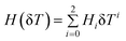
Gardas and Coutinho62 proposed a group contribution model for the isobaric expansivity (αP) at 298.15 K and 0.1 MPa, since the precision to which this property was known precluded a study of its temperature dependency as it is inferior to the experimental uncertainty.31 The model is based on 109 data points for 49 ILs with imidazolium, pyridinium, pyrrolidinium, piperidinium, phosphonium, and ammonium cations with 19 different anions. The average deviation reported is of the order of 1.98%, with a maximum deviation of 7%. From these, about 40.4% of the estimated refractive indices were within a deviation of 0–1%, and 36.7% were within 1–3%.
Preiss et al.47 proposed the following correlation for the isobaric expansivity:
 | (20) |
Here c = 0.0001747 K−1, d = 0.0008028 K−1 and V0 = 1 nm3. The molar volumes (Vm) used in the correlation are estimated by a computational method (BP86/TZVP + COSMO). Unfortunately the model has not been directly tested by the authors against experimental data.
3. Heat capacity
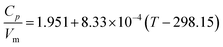
The near constancy of the volume specific heat capacity is well established, and is the basis of the Dulong–Petit law. Gardas and Coutinho64 produced the first report that ILs also obey this behaviour, showing that at 298.15 K| Cp = (1.9516 ± 0.0090)Vm | (21) |
with Cp in J mol−1 K−1 and with the molar volume Vm in cm3 mol−1, obtained from Ye and Shreeve.27 This correlation could describe the behaviour of approximately 20 ILs, with an average deviation of 1.15%, the largest deviation being less than 3.5%. Similar results using different databases have also been reported by other authors. Krossing and co-workers47 showed that a linear correlation with the molar volumes obtained from COSMO-RS could be proposed as
| Cp = 1169 Vm + 47.0 | (22) |
Since the database used is essentially the same as the one used by Gardas and Coutinho,64 the larger deviations of 5.5% must result from a worse description of the molar volume by the COSMO-RS approach used.
Paulechka et al.65 confirmed the results reported by Gardas and Coutinho64 and proposed an extension of this model with a dependency on temperature
 | (23) |
valid up to 350 K. The standard error of regression is 0.03 J K−1 cm−3 and the largest deviation is 4.9%.
Recently, Glasser and Jenkins66 seem to have rediscovered this concept and proposed another correlation for heat capacities at 298.15 K based on molecular volumes. The correlation and its results are very similar to those previously reported.
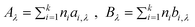
In one of the first works dealing with the measurement and modelling of the heat capacity of ILs, Waliszewski and co-workers67 used an additive group contribution method proposed by Chueh and Swanson68 based on the assumption that the heat capacity equals the sum of individual atomic-group contributions. The group contribution method was built based on data for molecular liquids, for which the agreement between experimental and estimated Cp values was generally within 2–3%, but for ILs the estimated Cp values are approximately 12% higher than experimental values.
Gardas and Coutinho64 proposed a group contribution method for the estimation of the heat capacities of ILs based on the Ruzicka and Domalski69,70 approach. This uses a second-order group additivity method for the estimation of the liquid heat capacity, applying a group contribution technique to estimate the parameters A, B, and D in
 | (24) |
where R is the gas constant and T is the absolute temperature. The group contributions used to calculate the parameters A, B,and D are obtained from the following relations:
 | (25) |
Here ni is the number of groups of type i, k is the total number of different types of groups, and the parameters ai, bi, and ci were reported for 4 cation families and 6 anions. This method allows the estimation of heat capacities of ILs as a function of temperature over wide temperature ranges (196.36–663.10 K). This model was applied to about 2400 data points for 20 different ILs, with an average deviation of 0.36% and a maximum deviation of less than 2.5%. From these values, 51.4% of the estimated heat capacities were within an absolute deviation of 0.00–0.20%, 27.1% were within 0.20–0.50%, 11.6% were within 0.50–1.0% and only 9.8% of the estimated heat capacities had a deviation larger than 2%. In almost all cases where the experimental uncertainty is provided in the original reference, the deviations in the predicted heat capacities are less than the assigned experimental uncertainties.
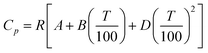
Ge et al.71 reported an extension of the Joback72,73 group contribution method for the estimation of the ideal gas heat capacity as a tool to predict the liquid heat capacity of ILs. The approach uses the equation
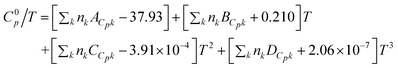 | (26) |
where ACpk, BCpk, CCpk, and DCpk are group contribution parameters, nk is the number of groups of type k in the molecule and T is the temperature in K, to estimate the ideal gas heat capacity of ILs. By applying the principle of corresponding states (CST) it is possible to use the ideal gas heat capacity, along with other thermodynamic properties of the component, to estimate the liquid heat capacity, using the following equation:73
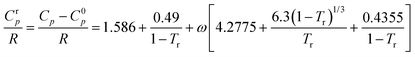 | (27) |
Here, R, Tr and ω are the gas constant, reduced temperature and acentric factor, respectively. Therefore, to enable the estimation of IL heat capacities, it is necessary to know (or be able to estimate) the boiling points and the critical properties of the ILs, which is a major drawback of this approach as these values are not known for ILs. For that purpose the model relies on the estimation of the critical properties proposed by Valderrama and Robles.51 This model shows an average deviation of 2.9% for 961 heat capacity experimental data points from 53 ILs studied.
These two group contribution methods had their parameter tables extended for amino acid based ILs by Gardas et al.74 Soriano et al.75 proposed a new version of the Gardas and Coutinho model with a parameter table with parameters A, B, and C (equivalent to D on the Gardas and Coutinho approach) for each individual cation and anion, instead of a group contribution model. Parameters for 10 cations and 14 anions are reported. The heat capacity of the IL is estimated as:
| Cp = Cp,cation + Cp,anion | (28) |
The agreement between the predicted heat capacity values and those from the literature is generally good, with deviations that range from 0.003–2.16% and an average deviation of 0.34% for all of the 2414 data points considered in the parameter estimation. The prediction of the heat capacity for 735 data points of another 9 ILs not used in the correlation had an average deviation of 1.81%.
Valderrama and co-workers48 proposed a method for the estimation of the heat capacity based on the so-called mass connectivity index, λ. The authors assume that the temperature dependency of the heat capacities have a linear dependency on this index, estimated by a group contribution approach, where
| Cp = Cp0 + λ[c(T − T0) + d(T2 − T20)] | (29) |
and the parameters c = 0.4579 and d = −3.533 × 10⁻⁴ are obtained by regression of the experimental data for about 30 ILs. In their first report, Cp0 is the experimental value at a reference temperature, which limits the application of the model to new systems. In subsequent works76 they propose the estimation of the reference heat capacity by a group contribution method
| Cp(T) = ΣigiGi + A + Bλ + λ[CT + DT2] | (30) |
where the values of the groups (Gi) and of the constants A, B and C are calculated using a set of 469 data points for 32 ILs and 126 data points for 126 organic compounds. The model has 40 parameters and is reported to describe the heat capacity of ILs with an average deviation of 2.6%. Alternatively, they proposed elsewhere77 a method for the estimation of the reference heat capacity
| Cp0 = a + bVm + cλ + dη | (31) |
as function of the molar volume (Vm), the mass connectivity index (λ), and the ratio between the masses of the cation and the anion (η). The general model is:
| Cp = a + bVm + cλ + dη + λ[e(T − T0) + f(T2 − T20)] | (32) |
Here, a = 15.80, b = 1.663, c = 28.01, d = −7.350, e = 0.2530 and f = 1.372 × 10⁻³ are universal constants valid for any IL, and T0 is a reference temperature defined as 298.15 K. The equation parameters were estimated based on data for 33 ILs, and the model is reported to describe the experimental data within an average deviation of 2.1%.
Only Valderrama et al.78 used NN to describe heat capacities. They used 477 data points of heat capacity for 31 ILs to train the network. To discriminate amongst the different substances, the molecular mass of the anion and cation and the mass connectivity index were considered as independent variables. The architecture of the proposed NN model has three layers: 5 neurons in the input array, 10 neurons in the hidden layer, and 1 neuron in the output layer, (5,10,1). The ability of the network was evaluated in a test set with 65 data points for 9 ILs with an average deviation of 0.22% and a maximum deviation of 3.6%. Table 2 summarises the main characteristics of the different models.
| Model type | Parameters | T range/K | N ILs | %AD | Ref |
|---|---|---|---|---|---|
| a N ILs—number of ILs; b GC—group contribution model; c MCI—mass connectivity correlation | |||||
| Correlation | 298 | 20 | 1.15 | 64 | |
| Correlation | 298–350 | 19 | n.a. | 65 | |
| GCb | 12 parameters for 3 cations and 6 anions | 196–663 | 20 | 0.36 | 64 |
| GC | 17 parameters | 256–470 | 53 | 2.9 | 71 |
| GC | 10 cations and 14 anions | 188–453 | 32 | 0.69 | 75 |
| GC | 40 parameters | 250–426 | 32 | 2.6 | 48 |
| MCIc | 298.15 | 33 | 2.1 | 77 | |
4. Surface tension
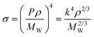
The estimation of surface tension is usually carried out by parachors, group contribution methods or the corresponding states theory. The parachor approach is based on an empirical formula proposed by MacLeod,79 expressing a temperature-independent relationship between the density ρ and the surface tension σ| σ1/4 = Kρ | (33) |
where K is a temperature-independent constant that is characteristic of the compound. Sugden80 proposed a modification to this expression that consists of multiplying each side of the expression by the molecular weight (MW) to give a constant KMW which he named parachor, Pch:
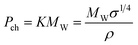 | (34) |
Sugden80 showed that the parachor is an additive property and that the parachor of a compound can be expressed as the sum of its parachor contributions. From the parachors it is possible to predict the surface tension of a compound if its density is known.
Mumford and Phillips81 and Quayle82 improved Sugden's parachor group contribution values for organic compounds, and recently Knotts et al.83 proposed a new group contribution correlation for the parachors, using the vast amount of physical data available in the DIPPR database. In this study, average deviations of 8.0% for multifunctional compounds were obtained, with maximum deviations of 34%.
Deetlefs et al.43 were the first to attempt the application of the Knotts et al.83 parachors to ILs. They calculated the parachors of ILs using the group contribution values estimated for non-ionic solvents and showed that the differences between the corresponding experimental and calculated values were small. Although the data used in their study was very limited, they postulated that the QSPR correlation based on neutral species could be used for ILs.
Using a database of 361 data points for 38 imidazolium-based ILs containing [BF4]−, [PF6]−, [Tf2N]− (bis(trifluoromethylsulfonyl)imide), [TfO]− (trifluoromethanesulphonate), [MeSO4]− (methylsulphate), [EtSO4]− (ethylsulphate), [Cl]−, [I]−, [I3]−, [AlCl4]−, [FeCl4]−, [GaCl4]− and [InCl4]− as anions, Gardas and Coutinho84 were the first to evaluate the quality of the surface tension estimates of ILs based on parachors calculated using the Knotts et al.83 method. For the 38 ILs studied, the overall deviation is 5.75%, with a maximum deviation of less than 16%, which is even lower than the value reported by Knotts et al.83 for multifunctional compounds. From these, 33.0% of the estimated surface tensions were within a deviation of 0–3.00%, 25.2% were within 3.00–6.00%, 24.1% were within 6.00–10.00%, and only 17.7% were higher than 10.0%. The deviations obtained were surprising, since the Knotts correlation for the parachors was developed for non-ionic compounds, without considering Coulombic interactions. While this work was focused on a database of only imidazolium compounds, the approach was later shown to apply as well to ILs of other cation families by Carvalho et al.85.
Gardas and Coutinho84 proposed yet another correlation for the surface tension of ILs based on the molecular volume of the ion pair. Combining the Eötvös86 and Guggenheim87 equations, and considering that the surface enthalpy varies within a very narrow range for most ILs, they proposed an equation relating the surface tension to the molecular volume
 | (35) |
where Vm is the molecular volume in Å3, obtained from Ye and Shreeve's work27 or calculated following Jenkins' procedure28, and d = 2147.761 ± 18.277 (mN m−1) Å2. This model gives a deviation of 4.50% for the surface tensions at 298.15 K of 47 data points of a total of 22 imidazolium-based ILs containing [BF4]−, [PF6]−, [Tf2N]−, [TfO]−, [MeSO4]−, [EtSO4]−, [Cl]− and [I]− as anions.
Gardas et al.46 proposed a correlation of parachors with molar volumes
| P = kV10/12m | (36) |
with k = 6.198, showing an average deviation of 2.17% for the parachors. Using this approach, the surface tensions can be estimated by
 | (37) |
Gardas et al.46 evaluated this correlation for 560 data points with an average deviation of 7.9% and a maximum deviation of 19.3%.
Ghatee et al.88 have shown that the relation between the viscosity and the surface tension
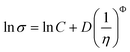 | (38) |
previously proposed for organic solvents89,90 also applies to ILs, where Φ is the universal exponent. However, contrary to other authors,90 they did not attempt to propose correlations for the C and D parameters limiting the predictive character of this approach.
The Corresponding States Theory (CST) has been widely used to correlate and predict thermophysical properties of organic and inorganic compounds. CST correlations for surface tensions have been proposed by several authors.91,92 However, the absence of critical properties limits the applicability of CST to ILs. In a recent work, Mousazadeh and Faramarzi93 proposed a CST correlation for the surface tension of ILs. In the absence of critical properties they chose to use the melting (Tfus) and boiling points (Tb) of ILs, along with the surface tension at the melting point (σm), to define their corresponding states correlation:
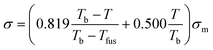 | (39) |
The deviations reported for surface tensions of 30 ILs used in the development of this correlation are of the order of only 3.0%, while the prediction errors for 4 ILs in a validation set are of 6.5%. The surface tensions estimated for 12 ILs using this approach are reported to be better than those of the Knotts et al.83 model studied by Gardas and Coutinho,84 with deviations of 2.4% instead of 6.7%. However, it should be noted that while the Knotts et al.83 model is fully predictive, the specific ILs used in this comparison were also present in the development of eqn (39). The major objections to this approach are that many ILs do not have a melting point, that the boiling temperatures of the ILs are as elusive as their critical temperatures, and consequently that the uncertainties associated with those estimates are necessarily very large. These problems severely limit the applicability of similar CST approaches to the prediction of the thermophysical properties of ILs.
The possibility of describing the surface tensions of [BF4], [PF6] and [Tf2N] ILs using the soft-SAFT EoS has been shown by Vega et al.14,59,60 Correlations for the EoS parameters are presented, establishing a predictive character in surface tension estimates using this methodology.
5. Speed of sound
The speed of sound seems to be a forgotten property of ILs. Despite its remarkable interest in the development of EoS for the description of ILs, the ILThermo10 database records speeds of sound for only 22 ILs, only two of which are not imidazolium. The data at pressures other than atmospheric pressure is scarcer still.Correlations for the prediction of speeds of sound are based on the Auerbach relation94
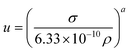 | (40) |
where a = 2/3, and σ and ρ are the surface tension in N m−1 and density in kg m−3, respectively. Gardas and Coutinho95 showed that while the original form described by eqn (40) could not be used to predict directly the speed of sound, a correlation between the experimental speed of sound, surface tension and density predicted by their models31,84 could be achieved. They showed that a linearization of the Auerbach relation
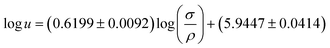 | (41) |
could provide an adequate description of the experimental data. Nevertheless, they chose to fit just one of the parameters in the Auerbach relation. By using a = 0.6714 ± 0.0002 in eqn (40), an overall relative deviation of 1.96%, with a maximum deviation of 5% was achieved for 133 data points of 14 imidazolium-based ILs, with 6 different anions available in the literature.
Recently, Singh and Singh96 reported a study for 3 ILs, where a similar approach was used but different coefficients are reported for the ILs studied.
6. Refractive index
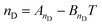
Little attention has also been given to the refractive index, both in terms of the experimental measurement of this property and the development of predictive models for it. This occurs despite the simplicity of its measurement and its interest as both an analytical tool and as a source of information on the intermolecular forces and behaviour in solution of ILs,97,98 as well as their free volumes43 (ILThermo10 reports the refractive index for only 28 ILs, only 4 of which are not imidazolium-based).The first approach in that direction was proposed by Deetlefs et al.,43 using the molar refraction RM, surface tension and parachor to estimate the refractive index nD:
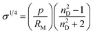 | (42) |
This approach was applied to a limited number of ILs with mixed success.
Gardas and Coutinho62 proposed a group contribution approach for the estimation of refractive indexes of ILs and their temperature dependency as:
 | (43) |
Here AnD and BnD can be obtained from a group contribution approach as
 | (44) |
where ni is the number of groups of type i and k is the total number of different groups in the molecule. The parameters ai,nD and bi,nD were proposed for imidazolium-based ILs with 7 different anions. The model was applied to 245 data points of 24 ILs available in the literature; the overall relative deviation is 0.18%, with a maximum deviation of the order of 0.6%. Of these, approximately 47.8% of the estimated refractive indexes are within a relative deviation of 0.00–0.10%, 45.7% within 0.10–0.50%, and only 6.5% of the estimated refractive indexes have a deviation larger than 0.5%.62 This model has been recently extended to other ILs by Soriano et al.99 and Freire et al.36 by proposing groups for nine other anions.
7. Transport properties
7.1 Viscosity
The viscosity is one of the most relevant and studied properties of ILs. It is thus not a surprise that it is also one of the properties for which more models have been proposed. While most of these models are of the QSPR or GC type, the first approaches to the description of this property were of a different type.Abbott100 suggested the use of the hole theory for the description of the viscosity of ionic and molecular liquids. The idea behind this model is that for an ion to move it must find a hole large enough to allow its movement. The probability P of finding a hole of radius r in a given liquid is given by:
 | (45) |
Therefore
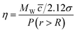 | (46) |
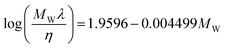
where MW is the molecular weight (for ionic fluids this is taken as the geometric mean), c is the average speed of the molecule [(8RT/πMW)1/2] and σ is the collision diameter of the molecule (4πR2). The application of this model to a range of liquids by Abbott100 showed that it is possible to predict the viscosities of these compounds with reasonable accuracy.
Bandres et al.101 adopted this approach to estimate the viscosity of 8 pyridinium ILs and obtained very large deviations from the experimental viscosity data. To improve the results they defined an effective IL radius, R*, which was fitted to the experimental viscosity data at 0.1 MPa. This approach yielded an average deviation of 4.5%. Further work along these lines may further improve the accuracy of the viscosity description by the hole theory.
Krossing and Slattery102 first remarked that the viscosity seems to have a linear dependence on the molecular volume of ILs. This work, latter expanded by Krossing and co-workers,29 was applied with success to some 30 ILs based on the [MFn], [N(CN)2] and [Tf2N] anions that were shown to follow an exponential decrease of the viscosity (η) with the molar volume (Vm) that could be described by the equation:
 | (47) |
This correlation is, however, anion-dependent and different a and b parameters are required for each anion, limiting the predictive ability of the approach. Moreover it only works for non-functionalized cations. Cation functionalization creates its own series in this correlation.103 Aiming at extending the applicability of this approach, Bogdanov et al.45 proposed an extension of their residual volume approach, presented above for the density, to the correlation of the viscosity according to:
| ln(ηX) = aβX + ln(η0) | (48) |
Here ηX is the viscosity of the X-substituted member of a series, a is the slope of the line, the intercept ln(η0) is the viscosity of the methyl-substituted member, and βX is the corresponding substituent constant, which are reported by the authors45 for four IL families. This model has, however, the same limitations identified for Krossing's approach.
Aiming at overcoming the previous limitations, Krossing and co-workers103 proposed new temperature-independent correlations, and one temperature-dependent correlation
 | (49) |
where η0 = 1 mPa s. The Gibbs solvation energy ΔG*,∞solv is calculated at the DFT-level (RI-)BP86/TZVP/COSMO, the molecular radius r*m is calculated from the molecular volume Vm of the ion volumes, and the symmetry number σ is obtained from group theory. The model was tested with some success on 81 ILs with a RMSE = 0.26.
Gardas and Coutinho104 proposed a group contribution approach where the viscosity of ILs is estimated using an Orrick–Erbar-type equation:105
 | (50) |
Here η is the viscosity in cP and ρ is the density in g cm−3, MW is the molecular weight and T is the absolute temperature. The group contribution parameters to calculate A and B for ILs are reported for 3 cation families and 8 anions. They are based on about 500 data points for 30 ILs, with an average deviation of 7.7% and a maximum deviation smaller than 28%. From the estimated viscosities, 71.1% present deviations smaller than 10%, while only 6.4% have deviations larger than 20%. Yet this model requires knowledge of the IL density, which some see as a drawback of the model.13 This problem was solved and the temperature description of the model was improved in a subsequent work,62 where a new group contribution model based on the Vogel–Tammann–Fulcher (VTF) equation was proposed:
 | (51) |
Here η is viscosity in Pa s, T is temperature in K, and Aη, Bη, and T0η are adjustable parameters. Gardas and Coutinho proposed a group contribution method to estimate Aη and Bη
 | (52) |

| (53) |
A different approach was proposed by Dutt and Ravikumar,107 with a reduced form of the Arrhenius model on a set of 29 ILs:
 | (54) |
Here ηR and TR denote the adimensional viscosity and temperature, defined as η/η323.15 and T/323.15, respectively, where η323.15 is the value of viscosity at 323.15 K. This model yields an average deviation of 16.7% for 244 data points. The ILs included in the correlation were imidazolium-, pyridinium- and ammonium-based. This approach was latter extensively tested by the authors108 but with deviations above 20% for the ILs studied.
Yamamoto109 reported the first QSPR study for the viscosity of ILs and proposed the following equation for its description:
| logη = 1.148 + 0.083(−0.0122Tref + 1)0.397 × (−0.0069[DP] + 1)0.664 × 0.1180[LUMO]+1)1.848 × (1.224[N1,charge] + 0.0762[N2,charge] + 1)1.213 × (0.1227[Area] + 0.5272[Volume] − 28.6399[Ovality] + 1)0.291 × (−0.066[TSFI] + 1.354[Cl] + 0.574[PF6] + 0.432[BF4] + 0.146[CF3SO3] + 1)1.575 | (55) |
This uses seven descriptors plus temperature and anion group contributions. In eqn (55)Tref (°C) is the temperature, [DP] (Debye) is the dipole moment, [LUMO] (eV) is the lowest unoccupied molecular orbital, [N1,charge] (and [N2,charge] if it exists) is the charge on the nitrogen atom. The values for these four descriptors are calculated by MOPAC.110 The [Area], [Volume], and [Ovality] are calculated by Chem3D.110 The anion parameters [TFSI], [Cl], etc., are set to 1 when the corresponding anion is present. This model provides a description of the temperature dependency of the viscosity with a reported correlation coefficient R2 of 0.9464 for 62 ILs.
One year later Yamamoto and co-workers111 proposed a new version of this model, essentially a non-linear group contribution model, valid for a larger number of cation families:
| logη = 0.562 + 1.368(0.036Tref +1)−4.040 × (0.729[alkylamine] + 1.131[pyrrole] + 2.048[piperidine] + 1.040[piridine] + 0.899[imidazole] + 0.619[pyrrazole])0.617 × (0.848[R1] + 0.465[R2] + 4.559[R3] + 2.442[R4] + 1)0.343 × (0.572[TSFI] + 2.602[Cl] + 2.464[Br] +1.289[PF6] + 1.046[BF4] + 0.791[CF3SO3] + 0.500[CF3BF3] + 0.580[C2F5BF3])0.725 | (56) |
Here Tref is the temperature in °C and R1, R2, R3, and R4 are the carbon number of the alkyl chain of the side chain. The value of the correlation coefficient R2 was 0.9419 for correlation and 0.9379 for prediction. The deviations are typically within 10% for correlation, but they increase considerably for predictions of [BF4], [PF6] and Cl based ILs.
For use in CAMD applications, a third model with descriptors based on just on the structure of the cation, side chain, and anion was also proposed by these authors:112
| logη = C0 + C1(C2Tref + 1)α × (ΣiCcation,iXcation,i+1)β × (ΣiCR,iXR,i + 1)γ × (ΣiCother,iXother,i + 1)δ × (ΣiCanion,iXanion,i + 1)ε | (57) |
This model consists of the terms of temperature, cation, the alkyl chain of the side chain attached in the cation, the other side chain, and anion. Using this model, it is possible to calculate the viscosity of ILs on the basis of just the structure of the ions. The estimation of the coefficients of eqn (57) for viscosity was performed using 300 experimental viscosity data points, with a temperature range of 0–80 °C. Parameters were reported by the authors for 5 cations and 13 anions. The correlation data set presents an acceptable R2 of 0.8971 but the prediction data set has an R2 of just 0.6226. The deviations of this model are significantly higher than the previous models by the same authors (up to 20%).
Yamamoto and co-workers113 reported a fourth QSPR correlation that is an enhanced version of their first proposal:109
| logη = 0.375 + 0.195((0.00285Tref + 1)−5.1120 × (0.714[DP] + 1)0.150 × (−0.0471[IP] − 0.0217[LUMO] + 1)−0.535 × (0.209[N1,charge] + 2.027[N2,charge] + 1)−0.195 × (0.578[Area] + 1.243[Volume] + 1)0.443 × (1.397[Ovality] + 1)−0.814 × (0.0282[TFSI] + 2.402[Br] + 2.887[Cl] + 0.538[BF4]0.255[CF3SO3] + 0.194[CF3COO] + 0.995[PF6] + 1.322[CH3COO] + 0.186[CF3BF3] −0.0199[C2F5BF3] + 0.0921[C3F7BF3] + 0.2005[C4F9BF3] − 0.165[EtOSO3] + 1.008[C4F9SO3] − 0.0375[CF3SO2NCOCF3] + 0.601[C3F7COO] + 1)0.676) | (58) |
This uses eight different descriptors plus temperature and anion group contributions. In eqn (58)Tref (°C) is the temperature, [DP] (Debye) is the dipole moment, [IP] (eV) is the ionization potential, [LUMO] (eV) is the lowest unoccupied molecular orbital, and [N1,charge] (and [N2,charge] if it is present) is the charge on the nitrogen atom. The values for these four descriptors are calculated by MOPAC.110 The [Area], [Volume] and [Ovality] are calculated by Chem3D.110 The anion parameters [TFSI], [Br], [Cl], etc., are set to 1 when the corresponding anion is present. This correlation presents an R2 of 0.9308 and a standard deviation (SD) of 0.143 for 329 data points.
Bini et al.114 studied various QSPR models for the viscosity based on the data measured by them for about 30 ILs. Each model is valid only at a single temperature (293 or 353) K. The descriptors were estimated using ab initio quantum mechanical calculations and the identification of the best correlation was carried with CODESSA. The best function identified, valid for 353 K, was
| η = (41.532 ± 6.5614) − (178.23 ± 20.11)[Nmax] − (0.7942 ± 0.08838)[PNSA-3] − (17.107 ± 4.073)[Cmax] | (59) |
where [Nmax] is the maximum electrophilic reactive index for an N atom, [PNSA-3] is the atomic charge weighted PNSA, and [Cmax] is the maximum atomic orbital electronic population. This three-descriptor model has an R2 of 0.8982 and F = 73.49. The correlations at 293 K are unsatisfactory. They found that cation–anion interactions play an important role for the viscosity, as indicated by the weight of the molecular descriptors of [FNSA-3] fractional PNSA and the maximum electrophilic reactive index for an N atom.
Recently Han et al.115 reported a new set of QSPR models for the viscosity of ILs. The descriptors are calculated by ab initio quantum mechanical calculations performed on isolated ions with Gaussian 03. The CODESSA package is then employed to derive the correlation equations between the viscosity and descriptors. They collected the viscosity data reported in the literature between 1983 and 2009 and split them into 4 data sets: the data of ILs based on [BF4]− (referred to as set A), [Tf2N]− (set B), [C4mim]+ (set C), and [C2mim]+ (set D). A correlation for each data set at 298 K and 1 atm, with 4 descriptors, is reported. The R2 values range from 0.92 to 0.97 and the authors claim that the largest deviation observed is of 13.6%. The models seems to be of good quality but their applicability is restricted to a limited range of compounds and they do not allow a description of the temperature dependency of the viscosity.
Mirkhani and Gharagheizi116 used a data set of 435 experimental viscosity data points for 293 ionic liquids covering 146 cations and 36 anions for the development of a new QSPR model that can be described by
| log(ηL) = 5.79187 + 0.56506 × ATS1v − 0.24393 × EEig02x − 0.88012 × C-038 + 0.2442 × ATS6m + 0.3117 × nNq + 0.51475 × C-008 − 0.146T | (60) |
This model used 348 data points as a training set and 87 data points as a validation set with an R2 of 0.8096 and F = 206.51, and uses 6 descriptors: ATS1v and ATS6m are derived from the Broto-Moreau autocorrelation116; EEig02x is the second eigenvalue of the “edge adjacency” matrix weighted by edge degrees; C-038 and C-008 are the atom-centered fragments for different groups and nNq represents the number of quaternary N that exists in the molecular structure of the cation. An average deviation of about 9% is reported.
Valderrama et al.117 also proposed the use of an NN to describe the viscosity of ILs. They used a training set composed of 327 data points of 58 ILs and used the molecular mass of the anion and of the cation, the mass connectivity index and the density at 298 K as independent variables. The NN proposed had an architecture of the type (5, 15, 15, 1) and was tested on a small set of 31 data points for 26 ILs with an average deviation of 1.68%. Billard et al.118 also proposed an NN to describe viscosity, but at the fixed temperature of 298 K; the predictions reported are very poor. Table 3 summarises the main characteristics of the different models.
| Model type | Parameters | T range/K | N ILs | %AD | Ref |
|---|---|---|---|---|---|
| a N ILs—Number of ILs. b *—Data points. | |||||
| Correlation | 253–373 | 81 | n.a. | 103 | |
| GC | 13 parameters for 3 cation and 8 anions | 293–393 | 29 | 7.7 | 104 |
| GC | 12 parameters for 3 cation families and 7 anions | 293–393 | 25 | 7.7 | 62 |
| Correlation | 273–363 | 29 | 16.7 | 107 | |
| QSPR | 7 descriptors, 16 parameters and 5 anions | 283–353 | 62 | 109 | |
| GC | 18 parameters for 6 cations and 8 anions | 293–363 | 146*b | 4.17 | 111 |
| QSPR | 27 parameters for 5 cations and 13 anions | 273–353 | 300*b | 112 | |
| QSPR | 8 descriptors, 18 parameters and 16 anions | 273–353 | 329*b | 113 | |
| QSPR | 3 descriptors and 4 parameters | 353 | 30 | 114 | |
7.2 Electrical conductivity
Four major approaches have been proposed for the development of predictive correlations of electrical conductivity for a wide range of IL families. The most basic approach is to relate it to the molar volume of the compounds. This approach proposed by Krossing and co-workers29 was applied with success to some 20 ILs based on the [MFn], [N(CN)2] and [Tf2N] anions, which were shown to follow an exponential decrease in their conductivity (κ) with the molar volume (Vm) described by the equation: | (61) |
Unfortunately this correlation is anion-dependent and different c and d constants are required for each anion, which limits the predictive ability of the approach. Moreover, it only works for non-functionalized cations. Cation functionalization creates its own series in this correlation.103 Aiming at extending the applicability of this approach, Bogdanov et al.119 proposed an extension of their residual volume approach, discussed above for density and viscosity, to the correlation of the electrical conductivities:
| lnκX = aβX + lnκ0 | (62) |
Here κX is the conductivity of the X-substituted member of a series, a is the slope of the line, the intercept lnκ0 is the conductivity of the methyl-substituted member, and βX is the corresponding substituent constant, which are reported by the authors.119 Parameters are reported for a vast number of IL families, but the model proposed is not able to overcome the limitations identified for Krossing's approach.
Since these models are not applicable to new ILs, Krossing and co-workers proposed various correlations to try to overcome this limitation.103 Using the same approach previously described for the viscosity they developed the equation
 | (63) |
where κ0 = 1 mS cm−1. The model presents a RMSE = 0.22 and R2 = 0.91. Based on the Stokes–Einstein and the Nernst–Einstein relations they also proposed the alternative correlation
 | (64) |
where κ0 = 1 mS cm−1, r0 = 1 nm, η0 = 1 mPa s, and ηcalc is the calculated viscosity according to the model proposed by them103 and described previously in the viscosity section. This correlation is reported to be slightly worse than the previous one (RMSE = 0.24; R2 = 0.90) but has one parameter less.
The second approach to the correlation of the electrical conductivity is based on the Walden rule120
| Λmη = const. | (65) |
relating the molar conductivity (Λm) with the viscosity (η). Its applicability to ILs has long been recognized.121
Galinski et al.122 showed that Λη values for a wide range of ILs are contained within a relatively narrow range of 50 ± 20 × 10−7 N s mol−1. Based on about 300 data points for 15 ILs Gardas and Coutinho62 proposed the following correlation, based on the Walden rule, to estimate the molar conductivity:
 | (66) |
Krossing and co-workers103 refitted this equation to a larger data set and the correlation obtained was
 | (67) |
that is essentially equivalent to the Gardas and Coutinho model.
QSPR type approaches have also been proposed by several authors for the correlation and prediction of electrical conductivity. The first was proposed in 2007 by Matsuda et al.112. The authors use a very complex and over parameterized equation
| κ = C0 + C1(C2TRef + 1)α × (ΣiCcation,iXcation,i + 1)β × (ΣiCR,iXR,i + 1)γ × (ΣiCother,iXother,i + 1)δ × (ΣiCanion,iXanion,i + 1)ε | (68) |
to describe the conductivities. This model has 8 fixed parameters plus the group parameters for 12 anions and 5 cation families. They evaluated the model against a database of about 200 data points where only the imidazolium-based ILs had a temperature dependency. The model seems to perform acceptably for conductivities larger than 6 mS cm−1, while it fails completely for low conductivities below 3 mS cm−1. Given the complexity of the model and the large number of parameters, this behaviour suggests a problem in the parameter estimation procedure.
Tochigi and Yamamoto113 proposed a QSPR approach to the description of conductivities. Their model
| κ = −0.496 + 1.001((0.00288[Tref] + 1)12.717 × (2.938[DP] + 1)−0.836 × (−0.577[IP] − 2.273[LUMO] + 1)0.361 × (3.756[N1,charge] + 2.205[N2,charge] + 1)4.174 × (0.100[Area] − 0.105[Volume] + 1)0.844 × (2.647[Ovality] + 1)−3.244 × (0.801[TSFI] − 0.317[Br] − 0.317[Cl] + 0.23[PF6] + 1.344[BF4] + 0.788[CF3SO3] + 0.992[CF3BF3] + 0.054[CH3COO] + 1.418[CF3BF3] + 1.279[C2F5BF3] + 0.812[C3F7BF3] + 0.331[C4F9BF3] + 0.142[EtSO4] − 0.157[C4F9SO3] + 0.883[CF3SO2NCOCF3] + 0.0369[C3F7COO] + 1)1.662) | (69) |
uses eight different descriptors plus temperature and anion group contributions. In eqn (69)Tref (°C) is the temperature, [DP] (Debye) is the dipole moment, [IP] (eV) is the ionization potential, [LUMO] (eV) is the lowest unoccupied molecular orbital, and [N1,charge] (and [N2,charge] if it is present) is the charge on the nitrogen atom. The values for these four descriptors are calculated by MOPAC.110 The [Area], [Volume], and [Ovality] are calculated by Chem3D.110 The anion parameters [TFSI], [Br], [Cl], etc., are set to 1 when the corresponding anion is present. This correlation presents an R2 of 0.9745, with a standard deviation of 0.630, an absolute average error of 0.457, a minimum error of −1.975 and a maximum error of 1.444 for 139 data points of ILs from 5 different cation families and 15 anions.
Bini et al.114 studied various QSPR models for the conductivity based on the data measured by them for about 30 ILs. As presented for the viscosity, each model is valid only at a single temperature (293 or 353 K) and the main descriptors are the principal moment of inertia, [A], the maximum partial charge, [Qmax], and the maximum 1-electron reactive index for a C atom, [Cmax]. The descriptors were estimated using ab initio quantum mechanical calculations and the identification of the best correlation was carried with CODESSA. The best function identified, valid for 353 K, was:
| κ = (9.8919 ± 1.1527) + (2.2095 × 10³ ± 1.9997 × 10³)[A] − (1.2174 × 10² ± 2.043 × 101)[Qmax] − (7.0256 × 101 ± 2.751 × 101)[Cmax] | (70) |
This three-descriptor model has an R2 of 0.9000 and F = 68.97.
Considering that the temperature dependency of the conductivity can be described by a VTF equation of the type
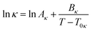 | (71) |
where Aκ, Bκ, and T0κ are adjustable parameters, Gardas and Coutinho62 proposed a group contribution method to estimate Aκ and Bκ according to
 | (72) |
 | (73) |
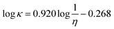
where ni is the number of groups of type i and m is the total number of different of groups in the molecule. The parameters ai,κ and bi,κ are reported for 4 cation families and 7 anions. Consistently with their approach to the description of the viscosity by the VFT equations,62 the T0κ value was fixed to a value identical to T0η (T0η = T0κ = 165.06 K). For 307 data points of 15 ILs the average deviation observed was 4.57%, with a maximum deviation of the order of 16%. From these values, 38.1% of the estimated electrical conductivities were within a relative deviation of 0–2)%, 25.7% within 2–5%, 22.8% within 5–10%, and only 13.4% of the estimated electrical conductivities showed deviations larger than 10%.
The fourth approach used for the description of the conductivity and transport properties in general, is the hole theory discussed above for the viscosity. Abbott123 was the first to apply this concept to the prediction of the conductivity of ILs. The approach assumes that the movement of ions in ILs is dependent on the availability of holes with a size equal to or larger than the fluid molecules. Since holes of adequate size are present in very low concentrations, the migration of holes is independent and can be described by the Stokes–Einstein equation. The following expression can thus be written for the conductivity:
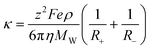 | (74) |
where z is the ion charge, F is the Faraday constant, e is the electronic charge, ρ is the density, MW is the molecular weight, and η is the viscosity of the IL, while R+ and R- are the ionic radii. Abbott123 applied this approach to about 30 ILs, obtaining a description of the data with an average deviation of 27.5%.
Zhao et al.124 proposed a modification to the Abbott approach by considering that the movement of the cation was made by a head dragging its tail. This means that the presence of a hole large enough to allow the movement of the head would be enough to promote the mobility of the charge and that the tail would then move to occupy the space left empty by the head. This approach yields the equation
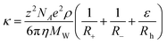 | (75) |
where Rh is the radius of the cation head and ε is the ratio of the surface areas of the head part and the whole cation. This new approach to the description of the conductivities by the hole theory enhances the quality of the description of the experimental data, allowing the reduction of the error to 2.2% at a fixed temperature of 298 K. Studies on the effect of the temperature on the quality of the predictions have not been reported. Table 4 summarises the main characteristics of the different models.
| Model type | Parameters | T range/K | N ILs | %ADb | Ref |
|---|---|---|---|---|---|
| a N ILs—Number of ILs. b %AD—Percentage average deviation. | |||||
| Correlation | 293–353 | 73 | 103 | ||
| Walden | 258–433 | 15 | 62 | ||
| QSPR | 25 parameters for 5 cation and 12 anions | 253–323 | 73 | 112 | |
| QSPR | 8 descriptors, 18 parameters and 16 anions | 243–338 | 73 | 0.457 | 113 |
| QSPR | 3 descriptors and 4 parameters | 293 or 353 | 30 | 114 | |
| GC | 13 parameters for 5 cations and 7 anions | 258–433 | 15 | 4.75 | 62 |
| Hole theory | 298 | 29 | 27.5 | 123 | |
| Hole theory | 298 | 24 | 2.2 | 124 | |
Hezave et al.22 also used an NN, but only for the description of the conductivity of the ternary systems IL–water–ethanol or IL–water–acetone. No attempts to describe the electrical conductivities of pure ILs have been hitherto made.
7.3 Thermal conductivity
ILs have been proposed as phase change materials,125–127 thermal fluids128–131 and hydraulic fluids.7,132 For these applications knowledge of the thermal conductivity is important for the correct choice of IL and equipment design. Despite their practical interest, thermal conductivities are among the less studied thermophysical properties of ILs with data reported at ILThermo10 for just 17 ILs, and most of the data from a single author.133 Recently these researchers74 reported a new set of data for another 11 ILs, based on amino acids along with new groups and parameters for the Gardas and Coutinho62 group contribution model for the thermal conductivity described below.Tomida et al.134 reported in 2007 some of the first data on the thermal conductivity of ILs and attempted to describe these by the Mohanty135 relationship
 | (76) |
but with very poor results. Based on their own data, the authors proposed a correlation based on the Mohanty relationship as
 | (77) |
valid for ILs and n-alkanes.
Froba et al.136 gathered new thermal conductivity data for a series of 10 ILs where they tested the correlation proposed by Tomida et al.,134 reporting that it seems to work only for a limited number of anions. After trying a number of empirical correlations, Froba et al.136 proposed
 | (78) |
where the parameters A = 0.1130 g cm−3 W m−1 K−1 and B = 22.65 g2 cm−3 W m−1 K−1 mol−1 were obtained by least-squares fitting of their data at a temperature of 293.15 K and atmospheric pressure. This correlation provides a maximum relative deviation of 10% for the data used in its development.
The only predictive model proposed for the thermal conductivity is a group contribution model proposed by Gardas and Coutinho.62 Based on the experimental data behaviour,74,136 it assumes that the thermal conductivity decreases linearly with temperature and thus could be described as
| λ = Aλ − BλT | (79) |
where T is the temperature in K, and Aλ and Bλ are fitting parameters that can be obtained from a group contribution approach as:
 | (80) |
Here ni is the number of groups of type i and k is the total number of different groups in the molecule, and the parameters ai,λ and bi,λ are proposed for three cations and six anions. For 107 data points of 16 ILs the average deviation is 1.1%, with a maximum deviation of 3.5%. Recently, Gardas et al.74 proposed seven new groups for amino acids and reported their values, extending the applicability of the model.
7.4 Self Diffusion coefficients
Very little attention has been paid so far to the self diffusion coefficients (D) of ILs. Few data are reported in the literature for this property and only two authors have addressed its modelling. Gardas and Coutinho62 proposed a correlation with viscosity based on the Stokes–Einstein relation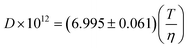 | (81) |
with an R2 of 0.997. However, the limited amount of data available precludes an extensive model evaluation.
Recently Borodin137 used molecular simulations to produce data to derive a correlation between the self diffusion coefficient and the enthalpy of vaporization (Hvap) according to the following relation:
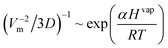 | (82) |
where α is a proportionality factor. Although the approach seems promising, the lack of experimental data for the enthalpy of vaporization did not allow the development of a final version of this correlation.
8. VLE properties
One of the most striking characteristics of ILs is their very low volatility. This creates a window of opportunity for their application but also limits their use in systems where vapour–liquid equilibrium (VLE) would be relevant. Even when it is just of limited interest for the design of processes or products, the knowledge of the relevant VLE properties is valuable for the development of models and correlations for IL properties. However the determination of the vapour–liquid equilibrium properties is either extremely difficult (and thus potentially inaccurate), such as for the vapour pressure (pvap) and the enthalpy of vaporization (ΔHvap), or is simply forbidden territory as for the normal boiling temperature (Tb) and the critical temperature (Tc).1388.1 Enthalpy of vaporization
Paulechka et al.139 produced the first report of the measurement of vapour pressure and enthalpy of vaporization for an IL. In that work they proposed an additive scheme for the estimation of ΔHvap, based on the classification of effective atoms by type:| ΔHvap298 = 6.2nC + 5.7nD + 10.4nN − 0.5nF + 10.6nS | (83) |
Here ni is the number of atoms of the ith kind in a molecule or an ionic pair. Luo et al.140 reported deviations between this correlation and their enthalpies of vaporization for [Tf2N] based ILs of about 15%, and about twice as large for [beti]-based ILs.
In a subsequent work141 where vapour pressures measured by Knudsen's effusion and the enthalpy of vaporization derived from these data are reported for four ILs of the [Tf2N] family, the authors used the Fowkes approach142 to derive a correlation between the enthalpy of vaporization, the surface tension and the molar volume of ILs based on these four data points:
| ΔgiH0m = AσV2/3mN1/3A + B | (84) |
Here A = 0.01121 and B = 2.4 kJ mol−1. The correlation coefficient R2 was 0.94 and the authors claim that the equation has an uncertainty that does not exceed 2%, although it is based only on four data points. Verevkin, one of the model proponents, testing it against a set of data available at a later stage143 recognized that it underestimated the enthalpy of vaporization available by 10–20 kJ mol−1. Moreover, he recognized that this correlation seems to be very sensitive to the values of the surface tension used in the calculations. The vaporization enthalpy can vary by as much as 15–20 kJ mol−1 due to using surface tension values from different sources. To overcome this limitation, Verevkin143 proposed a simple additive approach based on the chemical formula and structure of the IL. The enthalpy of vaporization is thus the result of a contribution which comes from the constituent elements, and a correction due to the structure of the IL:
| ΔgiHm(IL) = ΣiniΔHi + ΣjnjΔHj | (85) |
Here ΔHi is the contribution of the ith element, ni the number of elements of the ith type in the IL, ΔHj the contribution of the jth structural correction, and nj the number of structural corrections of the jth type in the IL. The values of these contributions for 9 different elements or structures are fitted to the experimental data available compiled by the author for just 12 ILs and then tested with 3 others. Average deviations of 5% for the tested values were obtained.
Deyko et al.144 reported enthalpies of vaporization for a set of ionic liquids and a correlation based on the idea that the enthalpies of vaporisation can be decomposed into three components: the Coulombic interaction between the ions, and the van der Waals contributions from the anion and the cation. Using this approach a very good description of the enthalpies of vaporization reported is achieved. Deyko et al.145 reported a new set of data of enthalpies of vaporization and show that this approach could provide an adequate description of the experimental data.
Lee and Lee146 suggested the use of solubility parameters to the estimation of enthalpies of vaporization based on the definition of the cohesive energy density square root (CED)
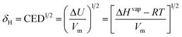 | (86) |
where ΔU, ΔHvap and Vm are the molar internal energy, the enthalpy of vaporization at 298 K and the molar volume, respectively.
Based on the solubility parameters estimated from the intrinsic viscosity, they estimated values of the enthalpy of vaporization that are 25% higher than those reported based on other methods.138 Recently Batista et al.147 made a detailed study of the solubility parameters of ILs, showing that they present a chameleonic behaviour that makes the direct estimation of the enthalpy of vaporization from the cohesive energies a delicate issue. Nevertheless, they show that the solubility parameters estimated from infinite dilution activity coefficients in non polar solvents produce good estimates of the high quality data for enthalpies of vaporization reported by Rocha et al.,148 suggesting that eqn (85) could be the basis for a method for the estimation of the enthalpy of vaporization of ILs. Zaitsau et al.149 made an extensive review of the data available and models proposed, and studied the dependency of the enthalpy of vapourization on various properties of ionic liquids, attempting to derive a correlation and showing that the task is probably not currently possible with the available information.
At present, the major problem with the application of these methods is the inadequacy of the experimental data in terms of both availability and quality to implement and validate predictive models for this property.
Although the discussion of molecular simulation methods is outside the scope of this review, it is nevertheless important to mention here the potential of COSMO-RS to provide a fast and reliable prediction of the enthalpy of vaporization.138,150
8.2 Normal boiling point temperatures
With boiling points, one enters what Rebelo named the “forbidden territory”,138 a realm of the virtual, since the ILs are not stable up to their boiling points. In one of the first works discussing the vapour–liquid properties of ILs, Rebelo et al.151 suggested the use of the Eötvös and Guggenheim equations to estimate the critical temperatures of the ILs, and from them to obtain a crude estimate of the boiling temperatures as Tb ∼ 0.6 Tc. Although this has been used later by several authors to report estimates of the boiling points of ILs from surface tension data, Rebelo acknowledges that “the method described in that paper allows only for rough estimates of both the critical and normal boiling temperatures”138 and should therefore be used with caution.Valderrama and Robles51 suggest using the modified Lydersen–Joback–Reid method for the estimation of the boiling temperatures of ILs as
| Tb = 198.2 + ΣnΔTbM | (87) |
using the parameter table proposed before for biomolecules152 with a few new parameters specific to ILs. The authors tested the validity of the proposed model on the prediction of the densities of ILs, as described below in the section addressing the critical properties. This approach was not primarily developed to estimate the boiling temperatures, but as a means to estimate the critical properties using the modified Lydersen–Joback–Reid method; it often produces estimates of the boiling temperatures that are unreasonably low. Given the absence of experimental data, a direct evaluation of the model is not possible.
8.3 Critical properties
The first approach aiming at the estimation of the critical properties was proposed by Rebelo et al.151 based on the Eötvös or the Guggenheim equations describing the temperature dependency of the surface tension of ILs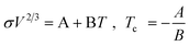 | (88) |
or
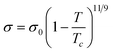 | (89) |
where σ is the surface tension, Tc is the critical temperature, and V is the orthobaric molar volume of the liquid. Both equations reflect the fact that σ becomes null at the critical point and are based on corresponding states principles. Although the authors acknowledge that this method “allows only for rough estimates of the critical temperatures”138 and should therefore be used with caution, recent results from molecular simulations by Rai and Maggin16 suggest that the critical temperatures estimated by these simple methods are in good agreement with those obtained by molecular simulation.
The alternative approach to the estimation of the critical properties of ILs is the work by Valderrama and Robles,51 which suggests applying the modified Lydersen–Joback–Reid method for their estimation:
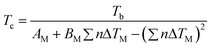 | (90) |
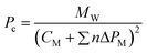 | (91) |
| Vc = EM + ΣnΔVM | (92) |
here n is the number of times that a group appears in the molecule, Tb is the normal boiling temperature, ΔTM is the contribution to the critical temperature, ΔPM is the contribution to the critical pressure, ΔVM is the contribution to the critical volume and AM, BM, CM and EM are constants and were calculated as AM = 0.5703, BM = 1.0121, CM = 0.2573, and EM = 6.75. The acentric factor is estimated from these relations as
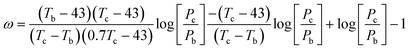 | (93) |
with Pb = 1 atm. The consistency of the estimated critical properties is assessed by using the densities of the ILs predicted by means of a correlation based on these properties. For 50 ILs the deviations vary between 1.6 and 20%, with an average deviation of 5.2%.51 The authors report in this first article the critical properties for 50 ILs and later published tables for hundreds of other ILs.153
Although the critical properties predicted by this approach have been widely used for the thermodynamic modelling of IL systems by equations of state154–160 or the estimation of other properties based on the corresponding states theory,54,71,161 the reader should be aware that these values are just parameters describing a virtual reality, often producing estimates that are physically unsound. Those interested in ongoing discussions about the validity of this approach should refer to the literature.162–164
8.4 Vapour pressures
Using the vapour pressures measured by Rocha et al.,148 Valderrama and Forrero165 showed that a cubic EoS of the Peng–Robinson type, using the concept of zero-pressure fugacity to describe these very low vapour pressures, could describe the experimental data with average deviations of less than 20%, with the best approach having deviations as low as 8%.9. Melting properties
Of all of the unusual properties displayed by ILs, the most differentiating is their low melting point, which forms the basis of the identity of this new family of salt compounds. Behind the large number of correlations for the melting properties of the ILs, in particular of their melting points, is the quest for understanding the characteristics that allowed the synthesis of liquid salts. The first works in this field were reported as early as 2002 and research is ongoing.9.1 Melting points
The most often adopted and successful approach for melting point predictions of ILs is the QSPR methodology. Using large training sets and bodies of descriptors, correlations for physical properties are derived, most often using the CODESSA code. This is probably the most difficult thermophysical property to predict and the correlation between experimental and predicted values for melting points is still incipient.The first approaches along these lines were reported by Katritzky et al.166 in 2002. Their correlations, in what is a recurrent approach for ILs, are only valid for a single IL family. The first attempt166 to describe the pyridinium bromides with a six-descriptor model achieved a correlation of R2 = 0.7883 and F = 73.24, with 126 ILs. Their second work167 addresses the imidazolium and benzilimidazolium bromides. A five-descriptor correlation based on 57 ILs was proposed, with R2 = 0.7442 and F = 29.67,
| Tfus = −(62.02 ± 6.16)[EHOMO–LUMO] + (96.58 ± 14.68)[J] + (1482.1 ± 232.1)[Pμ] + (667.4 ± 141.7)[Qmax,N] − (8.17 ± 1.89)[Emax,e–n,C] + (9.45 ± 3.56) | (94) |
were [EHOMO–LUMO] is the energy gap between the highest occupied molecular orbitals and the lowest unoccupied molecular orbitals, [Pμ] is the minimum atomic orbital electronic population, [Qmax,N] is the maximum partial charge for an N atom and [Emax,e–n,C] is the maximum electron–nuclear attraction for a C atom.
Eike et al.168 proposed another QSPR model for the 126 pyridinium bromide ILs studied by Katritzky et al.166 A correlation with five descriptors was proposed
| Tfus = 125.846 + 0.5773446[PNSA2] − 2273.22[FNSA3] − 104.034[BIC] + 254.703[RNCG] − 74.3734[RPCS] | (95) |
with an R2 of 0.790. As in the work by in Katritzky et al.166 the descriptors used stress the importance of electronic and symmetry effects. Four of the descriptors, [PNSA2], [FNSA3], [RNCG] and [RPCS], are charged partial surface area descriptors while the bonding information content [BIC] weakly indicates that a more complex (asymmetric) molecule should have a lower melting point. Their model, based on 75 tetra alkyl ammonium bromides:
 | (96) |
uses only topological descriptors: ([3χc − 3χVc] is the difference between the standard third order connectivity index (3χc) and the valence modified third order connectivity index (3χVc), [VIMadi] is the total information content on the adjacency magnitude, [CIC] is the complementary information content, 2χV is the valence-modified connectivity for two bond paths or three atoms in a row and [Φ] is the Kier flexibility index) and has R2 = 0.775. For (n-Hydroxyalkyl)-trialkyl-ammonium bromides they proposed yet another correlation
 | (97) |
based again on electronic descriptors (1χVp, 2χVp and 3χVp are Kier–Hall valence modified path connectivity indexes, [IC] is the information content and [SC1] counts the number of bonds present in a molecule), with R2 = 0.766. The prediction errors for compounds not included in the training sets can be as large as 70 K and the differences, for the same compound, between the various correlations proposed can be larger than 100 K.
Trohalaki and co-workers studied 1-substituted 4-amino-1,2,4-triazolium bromide and nitrate salts as energetic ILs, proposing QSPR correlations for the measured melting points of these compounds in two different publications.26,169 Since the database and the methodology are identical, and the results reported on the Energy & Fuels article26 are better, only these are here reviewed. For the melting points of the bromide salts they proposed
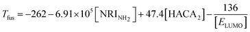 | (98) |
where [NRINH2] is the nucleophilic reactivity index for the amine nitrogen, [HACA2] is the area weighted surface charge of hydrogen-bond acceptor atoms, and [ELUMO] is the energy of the lowest unoccupied molecular orbital. This correlation, based on 13 ILs, has an R2 = 0.914 and F = 31.9. Their correlation for nitrates is the first for non halogenated salts. Based on data for 13 salts the correlation reported is
| Tfus = 284 − 214[HDCA12] − 3.94 × 10⁴[NRImin,c] + 3.16 × 10³[FHDCA] | (99) |
where [HDCA1Z] and [FHDCA] are measures of the hydrogen- bond-donating ability of the cation, and [NRImin,C] is the minimum [NRI] for a carbon atom. This model has R2 = 0.933 and F = 41.5.
Sun et al.170 proposed the first correlations for BF4 and PF6 imidazolium ILs. For BF4 ILs a three-descriptor correlation based on 16 ILs is proposed
| Tfus = −1704 −2641.2[EOnsager] + 16.146[Emin,e–e,C–C] + 4.5854[HDSAQ–C] | (100) |
with a R2 = 0.9047 and a F = 37.99, corresponding to an average deviation of 14 K and a relative error of 5%. Here the most important descriptor is [HDSAQ–C], which represents the H-donors surface area; [EOnsager] = (ε − 1)μ2/(2ε + 1), is the image of the Onsager–Kirkwood solvation energy, where ε is the macroscopic dielectric constant of the solvent where experimental data are obtained and μ is the total dipole moment of the molecule. [Emin,e–e,C–C] is the minimum e–e repulsion for a C–C bond, which relates to the conformational (rotational, inversional) changes or atomic reactivity in the molecules.
For the 25 PF6 ILs a six-descriptor correlation is required
| Tfus = −13936 + 22.418[Emin,e–e,C–C] + 819.81[Emax,R,C,C–H] + 8861.6[qmin,H] − 11.4[RNCSQ–C] + 2410.8[PN] − 299.01[BCmax,MO] | (101) |
with a R2 = 0.9207 and a F = 34.85, corresponding to an average deviation of 9.5 K and a relative error of 3.3%. Here [Emax,R,C–H] is the maximum resonance energy for a C–H bond which relates to the formation of hydrogen bond; [qmin,H] is the minimum partial charge for an H atom, reflecting the charge distribution of an H atom; [PN] is the maximum bond order of an N atom which is a valency-related descriptor describing the strength of intramolecular bonding interactions, including multipole interactions involving the N atoms of the imidazolium ring; [RNCSQ–C] is the relative negative charged surface area, and deals with the features responsible for polar interactions between molecules; and [BCmax,MO] is the maximum bonding contribution of a molecular orbit belonging to the atoms B and C in the molecule.
Yamamoto109 reported another correlation for 21 BF4 based ILs with an R2 = 0.837
| Tfus = 31.963 + 1.381(7.152[DP] + 1)−0.2027(6.750[LUMO] + 1)1.7363(1.723[N1,charge] + 3.779[N2,charge] + 1)2.0809(0.333[Area] + 2.180[Volume] − 4.409[Ova] + 1)−0.0715(−4.444[Hmax] + 1)0.6463(−0.260[Dis] + 1)0.7180(0.0730[Sym] + 1)1.2695 | (102) |
that uses ten descriptors where [DP] (Debye) is the dipole moment, [LUMO] (eV) is the lowest unoccupied molecular orbital, [N1,charge] (and [N2,charge] if it exists) is the charge on the nitrogen atom. The values for these four descriptors are calculated by MOPAC.110 The area, volume, and ovality are calculated by Chem3D.110 [Hmax] is the charge of the most positively charged hydrogen in the cation, [Dis] is the nitrogen and hydrogen atoms connected to the most positive carbon bond, and [Sym] is the symmetry around the nitrogen atom. Yamamoto was the first to attempt the development of a QSPR correlation for a broad range of cations and anions. The correlation proposed
| Tfus = 4.967 + 119.985(0.00813[DP] + 1)−3.2961(2.827[LUMO] + 1)0.3262 × (0.406[N1,charge] + 0.139[N2,charge] − 41.056[Hmax] + 1)1.7334 × (−0.0441[Area] + 0.0411[Volume] + 2.856[Ova] + 1)0.0497 × (−0.185[Dis] + 1)0.4598(0.555[Sym] + 1)0.2209 ×(−0.263[TSFI] + 0.189[Br] + 0.203[Cl] − 0.00309[PF6] − 0.163[BF4] − 0.225[CF3SO3] + 1)0.4923 | (103) |
uses 10 descriptors plus anion group contributions. The anion parameters [TFSI], [Br], [Cl], etc., are set to 1 when the corresponding anion is present. This model provides a description of the melting temperatures with a reported R2 of 0.61 for 60 ILs with 6 different anions.
Lopez-Martin et al.171 reported a correlation for 1-ethyl-3-methyl imidazolium-based ILs combined with 22 different anions, with 9 descriptors that present an R2 = 0.955. A second correlation for a set of 62 ILs (22 different cations and 11 different anions) is proposed based on six descriptors, with R2 = 0.869. The most important descriptors used on these correlations are related to size, symmetry, and charge distribution in either the cation or the anion. The authors also call the attention to the fact that the data sets are far from perfect because of polymorphism, impure ILs, and experimental confusion between glass transition temperatures and melting points, which makes the development of reliable regressions difficult.
Another correlation for various families of bromide ILs (including pyridinium, imidazolium, benzimidazolium, and 1-substituted 4-amino-1,2,4-triazolium) was proposed by Ren et al.172 Using the CODESSA descriptors and a PCA analysis, the best correlation reported (an eight-descriptor non linear model) has R2 = 0.804 and an AARD (%) of 18.39 for the training set. For the validation set the predictive results had R2 = 0.810 and an AARD (%) of 17.75. This model can correctly predict 42.59% of the data in the training set and 34.72% of the data in the test set, respectively, with the absolute value of the predicted error below 15 K. It predicts 73.15% and 72.22% of the compounds for the training and test sets, respectively, within an error of 30 K.
Yet another QSPR model for imidazolium bromide and chloride ILs was proposed by Yan et al.173 The model described by
| Tfus = 143.48[κ − 2] − 163.96[χ(1)] + 136.18[χ(3)V] − 54.47[E − SssCH2] + 571.66 | (104) |
presents R2 = 0.88 and F = 64.03for a training set of 50 ILs, with an average deviation of 17 K and a relative error of 4.6%. In this correlation the [κ−2] descriptor is the second order Kier shape index descriptor; [χ(1)] is first-order Kier and Hall connectivity index, representing information on the bonds that connect the skeletal atoms of the substituted group on the N atom of the imidazolium ring; [χ(3)V] is the third-order Kier and Hall valence-modified connectivity index, and [E − SssCH2] (E-state keys sums) descriptor is the sum of electrotopological state for a carbon bonded to two hydrogens and two bonds.
An exhaustive study of QSPR models for melting points was reported by Varnek et al.174 Here the authors used multiple approaches to perform QSPR modelling of the melting point of a structurally diverse data set of 717 bromides of nitrogen-containing organic cations. They tested several types of descriptors along with several popular machine learning methods such as associative neural networks (ASNN), support vector machines (SVM), k-nearest neighbours (k-NN), modified versions of the partial least-squares analysis (PLSM), back propagation neural networks (BPNN), and multiple linear regression analysis (MLR). They concluded that for the full set, the accuracy of the predictions does not significantly change as a function of the type of descriptor. Among the 16 types of developed structure-melting point models, nonlinear SVM, ASNN, and BPNN techniques demonstrate slightly better performance over the other methods. The best results for the full data set have R2 = 0.63 and RMSE = 37.5 K of predictions calculated on independent test sets. Like Lopez-Martin et al.,171 the authors also claim that the moderate accuracy of the predictions can be related to the quality of the experimental data used as well as to difficulties in considering the structural features of the ILs in the solid state (polymorphic effects, eutectics and glass formation).
The two most recent contributions to the modelling of melting points use other approaches. Preiss et al.175 correlated the melting points of ILs using
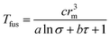 | (105) |
where the site symmetry σ and the number of torsion angles τ are both determined individually for the cation and the anion and are used as their geometric mean, and the molecular volume is expressed in terms of the cubed molecular radius, r3m. The coefficients a, b and c depend on the training set used. Fair results are obtained for a training set of 24 aluminate and borate ILs with an R2 of 0.9103 and an average error of 21.1 K, while the most universal approach using a training set comprising 67 ILs of all types has R2 = 0.6746 and an average error of 36.4 K. An alternative correlation proposed by the authors uses two extra parameters
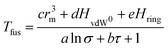 | (106) |
where the interaction enthalpies (HvdW0 and Hring) are calculated with COSMO-RS as the sum of the single-ion enthalpies in a 1:1 mixture of cation and anion at 25 °C. This correlation has R2 = 0.7987 and an average error of 24.5 K. Table 5 summarises the main characteristics of the different models.
| Model type | Structures | N DP | N ILs | R 2 | F | Ref |
|---|---|---|---|---|---|---|
| a N DP—Number of data points.b NILs—Number of ILs. | ||||||
| QSPR | Pyridinium bromides | 6 | 126 | 0.7883 | 73.24 | 166 |
| QSPR | Imidazolium and benzilimidazolium bromides | 5 | 57 | 0.7442 | 29.67 | 167 |
| QSPR | Pyridinium bromide | 5 | 126 | 0.790 | 168 | |
| QSPR | Tetra alkyl ammonium bromides | 5 | 75 | 0.775 | 168 | |
| QSPR | (n-Hydroxyalkyl)-trialkyl-ammonium bromides | 5 | 34 | 0.766 | 168 | |
| QSPR | 1-Substituted 4-amino-1,2,4-triazolium bromide | 3 | 13 | 0.914 | 31.9 | 26 |
| QSPR | 1-Substituted 4-amino-1,2,4-triazolium nitrate | 3 | 13 | 0.933 | 41.4 | 26 |
| QSPR | Imidazolium BF | 3 | 16 | 0.9047 | 37.99 | 170 |
| QSPR | Imidazolium PF | 6 | 25 | 0.9207 | 34.85 | 170 |
| QSPR | BF4 based | 10 | 21 | 0.837 | 109 | |
| QSPR | Not restricted | 16 | 60 | 0.61 | 109 | |
| QSPR | 1-Ethyl-3-methyl imidazolium | 9 | 22 | 0.955 | 171 | |
| QSPR | 1-Ethyl-3-methyl imidazolium | 6 | 62 | 0.869 | 171 | |
| QSPR | Bromide ILs | 8 | 0.804 | 172 | ||
| QSPR | Imidazolium bromide and chloride | 5 | 50 | 0.88 | 64.03 | 173 |
| QSPR | Bromides of nitrogen-containing organic cations | 717 | 0.63 | 174 | ||
| Correlation | Aluminate and borate | 3 | 24 | 0.9103 | 175 | |
| Correlation | Not restricted | 3 | 67 | 0.6746 | 175 | |
| Correlation | Not restricted | 5 | 67 | 0.7987 | 175 | |
| GC | Not restricted | 200 | 176 | |||
The only group contribution model for the melting points of ILs was proposed by Lazzús.176 The author used a data set of 200 ILs to estimate the group contributions, and 200 other ILs as a validation set. The approach used is based on the model of Joback and Reid,177 with anion and cation separation:
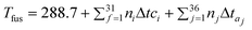 | (107) |
were ni and nj are the occurrence of the groups i and j in the IL, Δtc is the contribution of the cation group and Δta is the contribution of the anion group for the Tfus.
Despite its simplicity, this is the most general model yet reported for the melting temperatures of ILs and its deviations compares well with many of the specific models discussed above, with a relative deviation of only 7% for 400 ILs.
Given the complexity of the melting point description this has been a test field for unconventional models. This was the first property to be the object of an attempted description by an NN and for which more studies are available using this approach. Carrera and Aires de Sousa178 proposed as early as 2005 a model to describe the melting points of pyridinium bromides. Using DRAGON descriptors as the input, they applied CPG NN with R2 = 0.75 for the training set and values ranging from 0.58 to 0.76 for various testing sets. They later proposed yet another model for guanadinium ILs that was based on 92 descriptors, and produced average errors of 20–30 K.179
Torrecilla et al.180 achieved better results for imidazolium salts with various anions. With 9 cation and 5 anion descriptors as the input they studied a group of 97 ILs, from which 15% were randomly chosen as a validation set, achieving a description of these data with an average deviation of 1.3%. Besides the QSPR model described above, Yan et al.173 also reported the use of a back propagation NN for the prediction of the melting points of imidazolium bromides and chlorides, with deviations ranging from 5 to 9.3 K for the various sets tested.
9.2 Enthalpy of melting
Unlike melting temperatures, only a limited number of works addressed the correlation of melting enthalpies.125,126,175 The first work that considered this property, by Zhu et al.,126 reported the measurement of the melting properties for 10 different ILs and, along with other literature data, proposed a six-descriptor QSPR correlation for the heats of fusion:| ΔHfus = 112.82 − 3.1925[μ] − 7.3247[ELUMO] + 0.49747[S] − 0.23304[Volume] − 28.552[LH] + 0.17797[Ei] | (108) |
Here, the most important descriptor used is the cation–anion interaction energy of ILs ([Ei]), along with the dipole moment ([μ]), the volume ([Volume]), the surface area ([S]) and the shortest hydrogen bond distance ([LH]). The correlation is based on 44 ILs and has R2 = 0.9047 and F = 58.54, with a standard deviation of 4.797. The results on a prediction set of 10 ILs show deviations similar to those of the training set.
Bai et al.125 proposed another QSPR correlation based on a similar database of 40 ILs (of which 10 were used as a testing set) with only four descriptors:
| ΔHfus = −27.251 + 0.236[Volume] − 0.1[ELUMO] − 0.061[MW] + 0.971[μ] | (109) |
This correlation has R2 = 0.867 and F = 40.76, with a standard deviation of 3.482. They also proposed alternative correlations, valid for a more restricted group of ILs.
9.3 Glass transition temperatures
Only Lazzús181 reported a model for glass transition temperatures, using a group contribution model: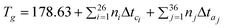 | (110) |
The groups were estimated based on information for 150 ILs, and a further 100 ILs were used as the test set. Groups are proposed for 9 different cation families, with an average deviation of 5% reported.
10. Discussion
Thermophysical properties models play a major role in chemical product and process modelling, both during their conceptual and operational phases, in assessing their impacts and understanding the corresponding life cycles. To help the interested reader navigate through the maze of models described, we have selected those that, in our opinion, are the most adequate to describe each of the properties considered. This selection is based on the models that currently present the broadest range of applicability and better accuracy, and is reported in Table 6. Unsurprisingly, the GC type of models dominate this landscape, which reflects not only the noteworthy flexibility of this methodology but also the greater exposure of researchers to it. Despite the low deviations reported by a number of NN models, we feel at present that they have not been sufficiently extensively tested to be recommended here. Most of the NN models reported come from Valderrama's research group. Given the promising results obtained so far, a further trial of structured nonlinear regression techniques, popular in other areas such as machine learning, is advisable (Fig. 1). The recent availability of implementations of these algorithms in computational environments such as Matlab/Octave, Mathematica, R, facilitates this task. A number of authors have made their models available either as on-line calculators or executable programs that can be easily obtained from them. Valderrama provides not only his NN codes50,78,117 but also his models to estimate the critical properties of ILs. Bogdanov's models45 are also freely available and the Gardas and Coutinho group contribution models are available as an on-line calculator.182| Property | Model | Type | Dev (%) | T range/K | p range/MPa |
|---|---|---|---|---|---|
| a GC—Group contribution model.b QSPR—Quantitative structure–activity relationship.c Corr—Correlation. | |||||
| Density | Paduszyñski and Domanska11 | GCa | 0.53 | 253–473 | 0.1–300 |
| Isothermal compressibility | Gardas and Coutinho62 | GC | 2.53 | 298.15 | 0.1 |
| Isobaric expansivity | Gardas and Coutinho62 | GC | 1.98 | 298.15 | 0.1 |
| Heat capacity | Paulechka et al.65 | Corrc | n.a. | 258–370 | 0.1 |
| Gardas and Coutinho64 | GC | 0.36 | 196–663 | 0.1 | |
| Surface tension | Knots et al. Parachors83,84 | GC+Corr | 5.75 | 268–393 | 0.1 |
| Speed of sound | Auerbach95,96 | Corr | 1.96 | 278–343 | 0.1 |
| Refractive index | Gardas and Coutinho36,62,99 | GC | 0.18 | 283–363 | 0.1 |
| Viscosity | Gardas and Coutinho104 | GC | 7.7 | 293–393 | 0.1 |
| Electrical conductivity | Walden rul62,103 | Corr | n.a. | 258–433 | 0.1 |
| Zhao et al.124 | Hole Theory | 2.2 | 298 | 0.1 | |
| Gardas and Coutinho62 | GC | 4.57 | 258–433 | 0.1 | |
| Thermal conductivity | Gardas and Coutinho62,74 | GC | 1.06 | 293–390 | 0.1 |
| Self diffusion coefficient | Stokes–Einstein62 | Corr | n.a. | 263–353 | 0.1 |
| Critical properties | Valderrama and Robles51 | GC | n.a. | — | — |
| Melting point | Lazzús176 | GC | 7 | 200–500 | 0.1 |
| Enthalpy of melting | Zhu et al.126 | QSPRb | 15 | — | 0.1 |
| Glass transition | Lazzús181 | GC | 5 | 150–350 | 0.1 |
The development of models for ILs cannot progress without the availability of good quality data. The situation today is far more favourable for some properties such as density and viscosity. There are, however, a number of other relevant properties to which little attention has been paid. The amount of available data for the heat capacity, speed of sound, surface tension, refractive index and thermal conductivity is too scarce. Experimental efforts aimed at the measurement of data for these properties, in particular for ILs with cations other than imidazolium, are required. The effect of pressure on the thermophysical properties is also only available for the density. Very little data is available for the viscosity and speed of sound, and we can only hope that this situation will be corrected in the near future.
In addition, despite the large number of attempts made to improve their description during the last decade, the prediction of melting properties remains elusive. Much of this can be blamed on the quality of the data, but important information concerning the nature of the solid phase itself seems to be missing in the models. Most models address the melting properties as if the solid was a liquid-like isotropic compound, not taking into account that each crystalline solid phase has its own characteristics. It will be difficult to develop better models for melting properties without explicitly considering the crystal structure of the solid phase.
Although the current popularity of GC methods means that extensive usage of this methodology will certainly be pursued in the future, this does not imply that its current practice is exempt from trouble. A first remark should be made on the need for more extensive quality validation of the models produced. While the reduced size of some data sets precludes the reservation of part of the data to build a test set for the model, alternative validation procedures such as cross-validation and various re-sampling schemes are available to solve this problem efficiently.183 Reporting the quality of the model only in terms of the quality of the fit obtained in a regression set is therefore clearly inappropriate. As discussed previously, an inaccurate characterization of the model accuracy makes the constraint-based selection of alternative ILs less proficient, and consequently the models less useful in practical applications.
An additional note should be made relative to the individual contributions identified as the regression coefficients during the development of the GC models: these methods were developed for non-ionic substances, where appropriate data sets can be chosen to evaluate uniquely each contribution. However, this is not necessarily the case with ILs. As a consequence, one of the basal assumptions of GC methods (individually recognizable contributions) can be questioned when applied to ILs. To illustrate this situation in a simple context, consider the case where a group of ILs is available, with cations A+, B+, C+, etc., and anions X−, Y−, Z−. If we measure a characteristic property P (e.g., independent of p and T), or a constant coefficient such as A, B or C in eqn (24) or (51), for the AX compound, using a GC additive model we would write
| P1 = a + x | (111) |
where a and x represent the group contribution coefficients (unknown). In this case we have one equation and two unknowns, and we need more data to determine a and x uniquely. If we replace the cation for B+ we get
| P2 = b + x | (112) |
and together with the new measurement we have also introduced one extra unknown (b), which still does not solve the problem uniquely. Continuing this process we are able to conclude that the individual contributions of the anion and cation cannot be completely separated, since there is always one degree of freedom left. This situation is different from that of non-ionic substances, where combinations like AA or XX are feasible, which allows the introduction of extra measurements (equations) without increasing the number of variables. Consequently, we can recognize that GC models of the above type do not necessarily have a unique set of constants that minimize the fitting error, but instead allow an infinite number of combinations of coefficients that describe the experimental data equally well. The exceptions to this observation occur when it is possible to previously measure (or fix) one of the coefficients used, as in the case of the volume or size parameters of the ion. While this fact does not affect the prediction capabilities of the GC methods, the modellers need to be aware of it, especially when comparing results from different authors or based on different data sets. The remaining degree of freedom needs to be fixed to produce a unique solution, and this can be solved using a number of distinct alternatives, e.g., by postulating a reference value for one of the coefficients or reformulating the regression objective as a minimum norm least-squares problem.
A final remark relative to the number of potential ILs: this has been repeatedly cited as 1018, wrongly attributing this value to Seddon.2,8 The correct citation (worth repeating here, since it has been wrongly quoted too often) is: “If there are one million possible simple systems, then there are one billion (1012) binary combinations of these, and one trillion (1018) ternary systems possible!!”.2 Although approximately 103 of these 106 simple compounds have been synthesized and about half of them are commercially available, Seddon's main point was that combinations of ILs could dramatically enlarge the range of physical properties achievable, thus enhancing the tunability of IL formulations. Studies of the thermophysical and transport properties of mixtures of ILs are surprisingly scarce given the body of data reported for mixtures with conventional solvents. Only a few systems for densities have appeared and some of the density models have been evaluated on their ability to describe these mixtures. Much effort from both experimentalists and modellers is thus required to fill this gap.
12. Conclusions
A review of predictive models for the thermophysical and transport properties of pure ILs was completed. It shows that while today there is abundance of data and models for some properties, such as viscosity and density, most properties have received much less attention from the ILs community than their practical importance in common chemical product and process applications would grant them. Limitations concerning the effects of pressure and the properties of IL mixtures were also highlighted. A recommendation was produced concerning the use of predictive models for each property studied. The best models were selected, taking into account the range of ILs for which they are applicable and the reliability of the estimates produced.References
- H. Olivier-Bourbigou, L. Magna and D. Morvan, Appl. Catal., A, 2010, 373, 1–56 CrossRef CAS.
- N. V. Plechkova and K. R. Seddon, Chem. Soc. Rev., 2008, 37, 123–150 RSC.
- V. Fábos, D. Lantos, A. Bodor, A. Bálint, L. T. Mika, O. E. Sielcken, A. Cuiper and I. T. Horváth, ChemSusChem, 2008, 1, 189–192 CrossRef CAS.
- D. J. Tempel, P. B. Henderson, J. R. Brzozowski, R. M. Pearlstein and H. Cheng, J. Am. Chem. Soc., 2008, 130, 400–401 CrossRef CAS.
- R. D. Rogers, K. R. Seddon, in Ionic Liquids IIIb: Fundamentals, Progress, Challenges, And Opportunities; Transformations And Processes, American Chemical Society, 2005 Search PubMed.
- Y. Chauvin, Angew. Chem., Int. Ed., 2006, 45, 3740–3747 CrossRef.
- R. Adler, Reports on Science and Technology, Linde Technology, Wiesbaden, 2006 Search PubMed.
- K. R. Seddon, The international George Papatheodorou Symposium: Proceedings, In, S. Boghosian, V. Dracopoulos, C. G. Kontoyannis and G. A. Voyiatzis (Ed.). 1999, 131–135 Search PubMed.
- A. J. Carmichael and K. R. Seddon, J. Phys. Org. Chem., 2000, 13, 591–595 CrossRef CAS.
- ILThermo - Standard Reference Data Program, National Institute of Standards and Technology, Gaithersburg, MD 20899, http://ilthermo.boulder.nist.gov/ILThermo..
- K. Paduszyński and U. Domańska, Ind. Eng. Chem. Res., 2012, 51, 591–604 Search PubMed.
- D. Rooney, J. Jacquemin, R. Gardas, Thermophysical Properties of Ionic Liquids. In Topics in Current Chemistry. Kirchner B (Ed.). Vol. 290, 2010 Search PubMed.
- S. Aparicio, M. Atilhan and F. Karadas, Ind. Eng. Chem. Res., 2010, 49, 9580–9595 CrossRef CAS.
- L. F. Vega, O. Vilaseca, F. Llovell and J. S. Andreu, Fluid Phase Equilib., 2010, 294, 15–30 CrossRef CAS.
- E. J. Maginn and J. R. Elliott, Ind. Eng. Chem. Res., 2010, 49, 3059–3078 CrossRef CAS.
- N. Rai and E. J. Maggin, J. Phys. Chem. Lett., 2011, 2, 1439–1443 Search PubMed.
- M. Smiglak, A. Metlen and R. D. Rogers, Acc. Chem. Res., 2007, 40, 1182–1192 CrossRef CAS.
- R. Gani, B. Nielsen and A. Fredenslund, AIChE J., 1991, 37, 1318–1332 Search PubMed.
- P. M. Harper, R. Gani, P. Kolar and T. Ishikawa, Fluid Phase Equilib., 1999, 158–160, 337–347 CrossRef CAS.
- N. Churi and L. E. K. Achenie, Ind. Eng. Chem. Res., 1996, 35, 3788–3794 Search PubMed.
- F. Friedler, L. T. Fan, L. Kalotai and A. Dallos, Comput. Chem. Eng., 1998, 22, 809–817 Search PubMed.
- A. Z. Hezave, M. Lashkarbolooki and S. Raeissi, Fluid Phase Equilib., 2012, 314, 128–133 Search PubMed.
- J. Gasteiger and J. Zupan, Angew. Chem., Int. Ed. Engl., 1993, 32, 503–527 CrossRef.
- J. Zupan, J. Gasteiger, in Neural networks for chemists; An Introduction, VCH PublishersNew York, NY, US, 1993 Search PubMed.
- C. M. Bishop, in Pattern Recognition and Machine Learning, Jorgda M, Kleinberg J & Schölkof B (ed.), Springer, 2006 Search PubMed.
- S. Trohalaki, R. Pachter, G. W. Drake and T. Hawkins, Energy Fuels, 2005, 19, 279–284 CrossRef CAS.
- C. Ye and J. M. Shreeve, J. Phys. Chem. A, 2007, 111, 1456–1461 CrossRef CAS.
- H. D. B. Jenkins, H. K. Roobottom, J. Passmore and L. Glasser, Inorg. Chem., 1999, 38, 3609–3620 CrossRef.
- J. M. Slattery, C. Daguenet, P. J. Dyson, T. J. S. Schubert and I. Krossing, Angew. Chem., Int. Ed., 2007, 46, 5384–5388 CrossRef CAS.
- J. A. Lazzús, J. Phys. Org. Chem., 2009, 22, 1193–1197 Search PubMed.
- R. L. Gardas and J. A. Coutinho, Fluid Phase Equilib., 2008, 263, 26–32 CrossRef CAS.
- A. J. L. Costa, J. M. S. S. Esperança, I. M. Marrucho and L. P. N. Rebelo, J. Chem. Eng. Data, 2011, 56, 3433–3441 Search PubMed.
- P. J. Carvalho, T. Regueira, L. M. N. B. F. Santos, J. Fernandez and J. A. P. Coutinho, J. Chem. Eng. Data, 2010, 55, 645–652 Search PubMed.
- C. M. S. S. Neves, P. J. Carvalho, M. G. Freire and J. A. P. Coutinho, J. Chem. Thermodyn., 2011, 43, 948–957 CrossRef CAS.
- C. M. S. S. Neves, M. L. S. Batista, A. F. M. Cláudio, L. M. N. B. F. Santos, I. M. Marrucho, M. G. Freire and J. A. P. Coutinho, J. Chem. Eng. Data, 2010, 55, 5065–5073 CrossRef CAS.
- M. G. Freire, A. R. R. Teles, M. A. A. Rocha, C. M. S. S. Neves, P. J. Carvalho, D. V. Evtuguin, L. M. N. B. F. Santos and J. A. P. Coutinho, J. Chem. Eng. Data, 2011, 56, 4813–4822 Search PubMed.
- F. S. Oliveira, M. G. Freire, P. J. Carvalho, I. M. Marrucho and J. A. P. Coutinho, J. Chem. Eng. Data, 2010, 55, 4514–4520 CrossRef CAS.
- C. L. Aguirre and L. A. Cisternas, Chem. Eng. Commun., 2012, 199, 283–289 Search PubMed.
- J. Jacquemin, R. Ge, P. Nancarrow, D. W. Rooney, M. F. Costa Gomes, A. A. H. Pádua and C. Hardacre, J. Chem. Eng. Data, 2008, 53, 716–726 CrossRef CAS.
- J. Jacquemin, P. Nancarrow, D. W. Rooney, M. F. Costa Gomes, P. Husson, V. Majer, A. A. H. Pádua and C. Hardacre, J. Chem. Eng. Data, 2008, 53, 2133–2143 Search PubMed.
- Y. Qiao, Y. Ma, Y. Huo, P. Ma and S. Xia, J. Chem. Thermodyn., 2010, 42, 852–855 Search PubMed.
- J. A. Lazzús, Chem. Eng. Commun., 2010, 197, 974–1015 Search PubMed.
- M. Deetlefs, K. R. Seddon and M. Shara, Phys. Chem. Chem. Phys., 2006, 8, 642–649 RSC.
- J. Palomar, V. R. Ferro, J. S. Torrecilla and F. Rodríguez, Ind. Eng. Chem. Res., 2007, 46, 6041–6048 CrossRef CAS.
- M. G. Bogdanov and W. Kantlehner, Z. Naturforsch., 2009, 64b, 215–222 Search PubMed.
- R. L. Gardas, D. W. Rooney and C. Hardacre, Fluid Phase Equilib., 2009, 283, 31–37 CrossRef CAS.
- U. P. R. M. Preiss, J. M. Slattery and I. Krossing, Ind. Eng. Chem. Res., 2009, 48, 2290–2296 CrossRef CAS.
- J. O. Valderrama and R. E. Rojas, Fluid Phase Equilib., 2010, 297, 107–112 Search PubMed.
- Y. Xiong, J. Ding, D. Yu, C. Peng, H. Liu and Y. Hu, Ind. Eng. Chem. Res., 2012, 50, 14155–14161 Search PubMed.
- J. O. Valderrama, A. Reátegui and R. E. Rojas, Ind. Eng. Chem. Res., 2009, 48, 3254–3259 Search PubMed.
- J. O. Valderrama and P. A. Robles, Ind. Eng. Chem. Res., 2007, 46, 1338–1344 CrossRef CAS.
- J. A. Lazzús, J. Taiwan Inst. Chem. Eng., 2009, 40, 213–232 Search PubMed.
- J. Lazzús, Int. J. Thermophys., 2009, 30, 883–909 CrossRef CAS.
- J. O. Valderrama and K. Zarricueta, Fluid Phase Equilib., 2009, 275, 145–151 CrossRef CAS.
- C. Shen, C. Li, X. Li, Y. Lu and Y. Muhammad, Chem. Eng. Sci., 2011, 66, 2690–2698 Search PubMed.
- J. Wang, Z. Li, C. Li and Z. Wang, Ind. Eng. Chem. Res., 2010, 49, 4420–4425 Search PubMed.
- S. Hosseini and Z. Sharafi, Ionics, 2011, 17, 511–516 Search PubMed.
- J. Abildskov, M. D. Ellegaard and J. P. O'Connell, Fluid Phase Equilib., 2010, 295, 215–229 Search PubMed.
- F. Llovell, E. Valente, O. Vilaseca and L. F. Vega, J. Phys. Chem. B, 2011, 115, 4387–4398 CrossRef CAS.
- F. Llovell, O. Vilaseca and L. F. Vega, Sep. Sci. Technol., 2012, 47, 399–410 Search PubMed.
- X. Ji and H. Adidharma, Chem. Eng. Sci., 2009, 64, 1985–1992 Search PubMed.
- R. L. Gardas and J. A. P. Coutinho, AIChE J., 2009, 55, 1274–1290 CrossRef CAS.
- R. L. Gardas, M. G. Freire, P. J. Carvalho, I. M. Marrucho, I. M. A. Fonseca, A. G. M. Ferreira and J. A. P. Coutinho, J. Chem. Eng. Data, 2007, 52, 80–88 CrossRef CAS.
- R. L. Gardas and J. A. P. Coutinho, Ind. Eng. Chem. Res., 2008, 47, 5751–5575 CrossRef CAS.
- Y. U. Paulechka, A. G. Kabo, A. V. Blokhin, G. J. Kabo and M. P. Shevelyova, J. Chem. Eng. Data, 2010, 55, 2719–2724 CrossRef CAS.
- L. Glasser and H. D. B. Jenkins, Inorg. Chem., 2011, 50, 8565–8569 Search PubMed.
- D. Waliszewski, I. Stepniak, H. Piekarski and A. Lewandowski, Thermochim. Acta, 2005, 433, 149–152 CrossRef CAS.
- C. F. Chueh and A. C. Swanson, Can. J. Chem. Eng., 1973, 51, 596–600 Search PubMed.
- V. Růžička and E. S. Domalski, J. Phys. Chem. Ref. Data, 1993, 22, 597–618 Search PubMed.
- V. Růžička and E. S. Domalski, J. Phys. Chem. Ref. Data, 1993, 22, 619–657 Search PubMed.
- R. Ge, C. Hardacre, J. Jacquemin, P. Nancarrow and D. W. Rooney, J. Chem. Eng. Data, 2008, 53, 2148–2153 CrossRef CAS.
- K. G. Joback, A Unified Approach to Physical Property Estimation using Multivariant Statistical Techniques. Thesis (M.S.)--Massachusetts Institute of Technology, Dept. of Chemical Engineering, 1984 Search PubMed.
- B. E. Poling, J. M. Prausnitz, J. P. O'Connell, in The Properties of Gases And Liquids, McGraw-Hill: New York, 2001 Search PubMed.
- R. L. Gardas, R. Ge, P. Goodrich, C. Hardacre, A. Hussain and D. W. Rooney, J. Chem. Eng. Data, 2010, 55, 1505–1515 Search PubMed.
- A. N. Soriano, A. M. Agapito, L. J. L. I. Lagumbay, A. R. Caparanga and M. Li, J. Taiwan Inst. Chem. Eng., 2010, 41, 307–314 Search PubMed.
- J. O. Valderrama, A. Toro and R. E. Rojas, J. Chem. Thermodyn., 2011, 43, 1068–1073 Search PubMed.
- J. O. Valderrama, G. Martinez and R. E. Rojas, Thermochim. Acta, 2011, 513, 83–87 Search PubMed.
- J. Valderrama, G. Martinez and C. Faúndez, Int. J. Thermophys., 2011, 32, 942–956 Search PubMed.
- D. B. Macleod, Trans. Faraday Soc., 1923, 19, 38–41 RSC.
- S. Sugden, J. Chem. Soc. Trans., 1924, 125, 1167–1177 RSC.
- S. A. Mumford and J. W. C. Phillips, J. Chem. Soc., 1929, 2112–2133 Search PubMed.
- O. R. Quayle, Chem. Rev., 1953, 53, 439–589 CrossRef CAS.
- T. A. Knotts, W. V. Wilding, J. L. Oscarson and R. L. Rowley, J. Chem. Eng. Data, 2001, 46, 1007–1012 CrossRef CAS.
- R. L. Gardas and J. A. P. Coutinho, Fluid Phase Equilib., 2008, 265, 57–65 CrossRef CAS.
- P. J. Carvalho, C. M. S. S. Neves and J. A. P. Coutinho, J. Chem. Eng. Data, 2010, 55, 3807–3812 CrossRef CAS.
- J. L. Shereshefsky, J. Phys. Chem., 1931, 35, 1712–1720 CrossRef CAS.
- E. A. Guggenheim, J. Chem. Phys., 1945, 13, 253–261 CAS.
- M. H. Ghatee, M. Zare, A. R. Zolghadr and F. Moosavi, Fluid Phase Equilib., 2010, 291, 188–194 CrossRef CAS.
- A. H. Pelofsky, J. Chem. Eng. Data, 1966, 11, 394–397 CrossRef CAS.
- A. J. Queimada, I. M. Marrucho, E. H. Stenby and J. A. P. Coutinho, Fluid Phase Equilib., 2004, 222–223, 161–168 CrossRef CAS.
- P. Rice and A. S. Teja, J. Colloid Interface Sci., 1982, 86, 158–163 CrossRef CAS.
- A. Queimada, I. M. Marrucho and J. Coutinho, Fluid Phase Equilib., 2001, 183–184, 229–238 Search PubMed.
- M. H. Mousazadeh and E. Faramarzi, Ionics, 2011, 17, 217–222 CrossRef CAS.
- N. Auerbach, Experientia, 1948, 4, 473–474 Search PubMed.
- R. L. Gardas and J. A. Coutinho, Fluid Phase Equilib., 2008, 267, 188–192 CrossRef CAS.
- M. P. Singh and R. K. Singh, Fluid Phase Equilib., 2011, 304, 1–6 Search PubMed.
- M. Tariq, P. A. S. Forte, M. F. C. Gomes, J. N. C. Lopes and L. P. N. Rebelo, J. Chem. Thermodyn., 2009, 41, 790–798 CrossRef CAS.
- K. Shimizu, M. Tariq, M. F. C. Gomes, L. P. N. Rebelo and J. N. C. Lopes, J. Phys. Chem. B, 2010, 114, 5831–5834 CrossRef CAS.
- A. N. Soriano, B. T. D. Jr and M. Li, J. Taiwan Inst. Chem. Eng., 2010, 41, 115–121 Search PubMed.
- A. P. Abbott, ChemPhysChem, 2004, 5, 1242–1246 CrossRef CAS.
- I. Bandrés, R. Alcalde, C. Lafuente, M. Atilhan and S. Aparicio, J. Phys. Chem. B, 2011, 115, 12499–12513 Search PubMed.
- I. Krossing and J. M. Slattery, Z. Phys. Chem., 2006, 220, 1343–1359 CrossRef CAS.
- P. Eiden, S. Bulut, T. Köchner, C. Friedrich, T. Schubert and I. Krossing, J. Phys. Chem. B, 2011, 115, 300–309 Search PubMed.
- R. L. Gardas and J. A. Coutinho, Fluid Phase Equilib., 2008, 266, 195–201 CrossRef CAS.
- R. C. Reid, J. M. Prausnitz, T. K. Sherwood, in The Properties of Gases and Liquids, McGraw-Hill, New York. 4th ed. 1987 Search PubMed.
- M. Tariq, P. J. Carvalho, J. A. P. Coutinho, I. M. Marrucho, J. N. C. Lopes and L. P. N. Rebelo, Fluid Phase Equilib., 2011, 301, 22–32 CrossRef CAS.
- N. V. K. Dutt and Y. V. L. Ravikumar, 3rd National conference on thermodynamics of chemical and biological systems, Nagpur, India, 2008, 166 Search PubMed.
- N. V. K. Dutt, Y. V. L. R. Kumar and K. Y. Rani, Fluid Phase Equilib., 2012 Search PubMed , submitted.
- H. Yamamoto, Journal of Computer Aided Chemistry, 2006, 7, 18–30 Search PubMed.
- Chem 3D, CambridgeSoft Corporation, 100 Cambridge Park Drive,Cambridge, MA 02140.
- H. Matsuda, H. Yamamoto, K. Kurihara and K. Tochigi, J. Comput. Aided Chem., 2007, 8, 114–127 Search PubMed.
- H. Matsuda, H. Yamamoto, K. Kurihara and K. Tochigi, Fluid Phase Equilib., 2007, 261, 434–443 Search PubMed.
- K. Tochigi and H. Yamamoto, J. Phys. Chem. C, 2007, 111, 15989–15994 Search PubMed.
- R. Bini, M. Malvaldi, W. R. Pitner and C. Chiappe, J. Phys. Org. Chem., 2008, 21, 622–629 Search PubMed.
- C. Han, G. Yu, L. Wen, D. Zhao, C. Asumana and X. Chen, Fluid Phase Equilib., 2011, 300, 95–104 Search PubMed.
- S. A. Mirkhani and F. Gharagheizi, Ind. Eng. Chem. Res., 2012, 51, 2470–2477 Search PubMed.
- J. Valderrama, J. Muñoz and R. Rojas, Korean J. Chem. Eng., 2011, 28, 1451–1457 Search PubMed.
- I. Billard, G. Marcou, A. Ouadi and A. Varnek, J. Phys. Chem. B, 2011, 115, 93–98 Search PubMed.
- M. G. Bogdanov, B. Iliev and W. Kantlehner, Z. Naturforsch., 2009, 64b, 756–764 Search PubMed.
- P. Walden, Z. Phys. Chem., 1906, 55, 207–249 Search PubMed.
- P. Wasserscheid, T. Welton, in Ionic Liquids in Synthesis, Verlag: Weinheim (Ed.), Wiley-VCH, 2003 Search PubMed.
- M. Galiński, A. Lewandowski and I. Stepniak, Electrochim. Acta, 2006, 51, 5567–5580 CrossRef CAS.
- A. P. Abbott, ChemPhysChem, 2005, 6, 2502–2505 CrossRef CAS.
- H. Zhao, Z. Liang and F. Li, J. Mol. Liq., 2009, 149, 55–59 CrossRef CAS.
- L. Bai, J. Zhu and B. Chen, Fluid Phase Equilib., 2011, 312, 7–13 Search PubMed.
- J. Zhu, L. Bai, B. Chen and W. Fei, Chem. Eng. J., 2009, 147, 58–62 Search PubMed.
- V. D. Bhatt, K. Gohil and A. Mishra, Int. J. ChemTech Res., 2010, 2(3), 1771–1779 Search PubMed.
- J. D. Holbrey, W. M. Reichert, R. G. Reddy and R. D. Rogers, Heat Capacities of Ionic Liquids and Their Applications as Thermal Fluids., ACS Symp. Ser., 2003, 856, 121–133 Search PubMed.
- B. Wu, R. G. Reddy, R. D. Rogers, Novel Ionic Liquid Thermal Storage for Solar Thermal Electric Power Systems. Proceedings of Solar Forum 2001, Solar Energy: The Power to Choose & April 21-25, 2001, Washington, DC, 2001 Search PubMed.
- J. F. Wishart, Energy Environ. Sci., 2009, 2, 956–961 RSC.
- M. E. Valkenburg, R. L. Vaughn, M. Williams and J. S. Wilkes, Thermochim. Acta, 2005, 425, 181–188 CrossRef CAS.
- W. Gu, H. Chen, Y. Tung, J. Meiners and S. Takayama, Appl. Phys. Lett., 2007, 90, 033505 CrossRef.
- R. Ge, C. Hardacre, P. Nancarrow and D. W. Rooney, J. Chem. Eng. Data, 2007, 52, 1819–1823 CrossRef CAS.
- D. Tomida, S. Kenmochi, T. Tsukada, K. Qiao and C. Yokoyama, Int. J. Thermophys., 2007, 28, 1147–1160 Search PubMed.
- S. R. Mohanty, Nature, 1951, 168, 42–42 Search PubMed.
- A. Froba, M. Rausch, K. Krzeminski, D. Assenbaum, P. Wasserscheid and A. Leipertz, Int. J. Thermophys., 2010, 31, 2059–2077 Search PubMed.
- O. Borodin, J. Phys. Chem. B, 2009, 113, 12353–12357 CrossRef CAS.
- J. M. S. S. Esperança, J. N. Canongia Lopes, M. Tariq, L. M. N. B. F. Santos, J. W. Magee and L. P. N. Rebelo, J. Chem. Eng. Data, 2010, 55, 3–12 CrossRef.
- Y. U. Paulechka, D. H. Zaitsau, G. J. Kabo and A. A. Strechan, Thermochim. Acta, 2005, 439, 158–160 CrossRef CAS.
- H. Luo, G. A. Baker and S. Dai, J. Phys. Chem. B, 2008, 112, 10077–10081 CrossRef CAS.
- D. H. Zaitsau, G. J. Kabo, A. A. Strechan, Y. U. Paulechka, A. Tschersich, S. P. Verevkin and A. Heintz, J. Phys. Chem. A, 2006, 110, 7303–7306 CrossRef CAS.
- F. M. Fowkes, J. Phys. Chem., 1963, 67, 2538–2541 CrossRef CAS.
- S. P. Verevkin, Angew. Chem., Int. Ed., 2008, 47, 5071–5074 CrossRef CAS.
- A. Deyko, K. R. J. Lovelock, J. Corfield, A. W. Taylor, P. N. Gooden, I. J. Villar-Garcia, P. Licence, R. G. Jones, V. G. Krasovskiy and E. A. Chernikova, Phys. Chem. Chem. Phys., 2009, 11, 8544–8555 RSC.
- A. Deyko, S. G. Hessey, P. Licence, E. A. Chernikova, V. G. Krasovskiy, L. M. Kustov and R. G. Jones, Phys. Chem. Chem. Phys., 2012, 14, 3181–3193 RSC.
- S. H. Lee and S. B. Lee, Chem. Commun., 2005, 3469–3471 RSC.
- M. L. S. Batista, C. M. S. S. Neves, P. J. Carvalho, R. Gani and J. A. P. Coutinho, J. Phys. Chem. B, 2011, 115, 12879–12888 Search PubMed.
- M. A. A. Rocha, C. F. R. A. C. Lima, L. R. Gomes, B. Schröder, J. A. P. Coutinho, I. M. Marrucho, J. M. S. S. Esperança, L. P. N. Rebelo, K. Shimizu and J. N. C. Lopes, J. Phys. Chem. B, 2011, 115, 10919–10926 Search PubMed.
- D. H. Zaitsau, K. Fumino, V. N. Emel'yanenko, A. V. Yermalayeu, R. Ludwig and S. P. Verevkin, ChemPhysChem, 2012 DOI:10.1002/cphc.201100879.
- M. Diedenhofen, A. Klamt, K. Marsh and A. Schafer, Phys. Chem. Chem. Phys., 2007, 9, 4653–4656 RSC.
- L. P. N. Rebelo, J. N. Canongia Lopes, J. M. S. S. Esperanca and E. Filipe, J. Phys. Chem. B, 2005, 109, 6040–6043 CrossRef CAS.
- V. H. Alvarez and J. O. Valderrama, Alimentaria, 2004, 254, 55–66.
- J. O. Valderrama, W. W. Sanga and J. A. Lazzús, Ind. Eng. Chem. Res., 2008, 47, 1318–1330 CrossRef CAS.
- P. J. Carvalho, V. H. Álvarez, J. J. B. Machado, J. Pauly, J. Daridon, I. M. Marrucho, M. Aznar and J. A. P. Coutinho, J. Supercrit. Fluids, 2009, 48, 99–107 CrossRef CAS.
- P. J. Carvalho, V. H. Álvarez, B. Schröder, A. M. Gil, I. M. Marrucho, M. Aznar, L. M. N. B. F. Santos and J. A. P. Coutinho, J. Phys. Chem. B, 2009, 113, 6803–6812 CrossRef CAS.
- P. J. Carvalho, V. H. Alvarez, I. M. Marrucho, M. Aznar and J. A. P. Coutinho, J. Supercrit. Fluids, 2009, 50, 105–111 CrossRef CAS.
- P. J. Carvalho, V. H. Álvarez, I. M. Marrucho, M. Aznar and J. A. P. Coutinho, J. Supercrit. Fluids, 2010, 52, 258–265 CrossRef CAS.
- S. Mattedi, P. J. Carvalho, J. A. P. Coutinho, V. H. Alvarez and M. Iglesias, J. Supercrit. Fluids, 2011, 56, 224–230 CrossRef CAS.
- V. H. Alvarez, R. Larico, Y. Ianos and M. Aznar, Braz. J. Chem. Eng., 2008, 25, 409–418 Search PubMed.
- J. O. Valderrama, A. Reategui and W. W. Sanga, Ind. Eng. Chem. Res., 2008, 47, 8416–8422 Search PubMed.
- R. L. Gardas, M. G. Freire, P. J. Carvalho, I. M. Marrucho, I. M. A. Fonseca, A. G. M. Ferreira and J. A. P. Coutinho, J. Chem. Eng. Data, 2007, 52, 1881–1888 CrossRef CAS.
- R. G. Jones, P. Licence, K. R. J. Lovelock and I. J. Villar-Garcia, Ind. Eng. Chem. Res., 2007, 46, 6061–6062 Search PubMed.
- J. O. Valderrama and P. A. Robles, Ind. Eng. Chem. Res., 2007, 46, 6063–6064 Search PubMed.
- J. O. Valderrama and R. E. Rojas, Ind. Eng. Chem. Res., 2009, 48, 6890–6900 CrossRef.
- J. O. Valderrama and L. A. Forero, Fluid Phase Equilib., 2012, 317, 77–83 Search PubMed.
- A. R. Katritzky, A. Lomaka, R. Petrukhin, R. Jain, M. Karelson, A. E. Visser and R. D. Rogers, J. Chem. Inf. Model., 2002, 42, 71–74 CrossRef CAS.
- A. R. Katritzky, R. Jain, A. Lomaka, R. Petrukhin, M. Karelson, A. E. Visser and R. D. Rogers, J. Chem. Inf. Model., 2002, 42, 225–231 CrossRef CAS.
- D. M. Eike, J. F. Brennecke and E. J. Maginn, Green Chem., 2003, 5, 323–328 RSC.
- S. Trohalaki and R. Pachter, QSAR Comb. Sci., 2005, 24, 485–490 Search PubMed.
- N. Sun, X. He, K. Dong, X. Zhang, X. Lu, H. He and S. Zhang, Fluid Phase Equilib., 2006, 246, 137–142 CrossRef CAS.
- I. López-Martin, E. Burello, P. N. Davey, K. R. Seddon and G. Rothenberg, ChemPhysChem, 2007, 8, 690–695 CrossRef CAS.
- Y. Ren, J. Qin, H. Liu, X. Yao and M. Liu, QSAR Comb. Sci., 2009, 28, 1237–1244 Search PubMed.
- C. Yan, M. Han, H. Wan and G. Guan, Fluid Phase Equilib., 2010, 292, 104–109 Search PubMed.
- A. Varnek, N. Kireeva, I. V. Tetko, I. I. Baskin and V. P. Solov'ev, J. Chem. Inf. Model., 2007, 47, 1111–1122 CrossRef CAS.
- U. Preiss, S. Bulut and I. Krossing, J. Phys. Chem. B, 2010, 114, 11133–11140 Search PubMed.
- J. A. Lazzús, Fluid Phase Equilib., 2012, 313, 1–6 Search PubMed.
- K. K. Joback and R. Reid, Chem. Eng. Commun., 1987, 57, 233–247 CAS.
- G. Carrera and J. Aires-de-Sousa, Green Chem., 2005, 7, 20–27 RSC.
- G. V. Carrera, L. C. Branco, J. Aires-de-Sousa and C. A. M. Afonso, Tetrahedron, 2008, 64, 2216–2224 CrossRef CAS.
- J. S. Torrecilla, F. Rodriguez, J. L. Bravo, G. Rothenberg, K. R. Seddon and I. Lopez-Martin, Phys. Chem. Chem. Phys., 2008, 10, 5826–5831 RSC.
- J. A. Lazzús, Thermochim. Acta, 2012, 528, 38–44 Search PubMed.
- P. J. Carvalho and J. A. P. Coutinho, ThermophIL - An Application for Ionic Liquids Property Estimation, http://path.web.ua.pt/thermophil,, 2012 Search PubMed.
- P. I. Good, in Resampling methods: a practical guide to data analysis, Birkhäuser, 2006 Search PubMed.
| This journal is © The Royal Society of Chemistry 2012 |