Reversible chemical storage of halogens in few-layer graphene

Abstract

Few-layer graphene can be chlorinated up to 56 wt.% by irradiation with UV light in a liquid chlorine medium. The chlorinated sample decomposes on heating or on laser irradiation releasing all the chlorine. Similar results have been obtained with the bromination of few-layer graphene.

---

Graphene, containing a two-dimensional network of sp²carbon atoms, possesses many novel physical and chemical properties.^1,2 In particular, the large π system of graphene participates in molecular charge-transfer with electron donor and acceptor molecules.^3,4 Thus, C₆₀ which is a good electron acceptor interacts with graphene through charge-transfer.⁵ Charge-transfer results in marked changes in the Raman spectrum of graphene. Graphene also interacts with metal nanoparticles giving rise to changes in the Raman spectrum.⁶ An unusual property of graphene discovered recently is its ability to store hydrogen.^7,8 Birch-reduction of few-layer graphene was found to give rise to hydrogenated graphene containing up to 5 wt.% of hydrogen. Interestingly, hydrogenated graphene decomposes on heating up to 500 °C or on laser irradiation, releasing all the hydrogen. This result demonstrates that the sp³ C–H bond of hydrogenated graphene can be considered to act as a reversible chemical storage of hydrogen. Recently, reversible fluorination of graphene has also been reported.^9–11 In the light of this observation, we felt that it would be of interest to carry out halogenation of graphene and examine the nature of the halogenated product. It would be interesting to explore whether halogenated graphene decomposes on heating or on laser irradiation. We have therefore carried out chlorination of graphene and examined the stability of the chlorinated product. We have also carried out a similar study on bromination of graphene.

We decided to carry out halogenation studies on few-layer graphene since the presence of more than one layer was found to favor the hydrogenation reaction. We have used graphene samples with 2–4 layers for the present study. The graphene (G) sample was characterized by employing transmission electron microscopy (TEM), atomic force microscopy (AFM), X-ray photoelectron spectroscopy (XPS), Raman spectroscopy and infrared spectroscopy (see experimental section for details). The Brunauer–Emmett–Teller (BET) surface area of the graphene was around 200 m² g⁻¹. The Raman spectrum showed the characteristic D (1323 cm⁻¹), G (1572 cm⁻¹), D′ (1600 cm⁻¹) and 2D (2641 cm⁻¹) bands.^12,13 The D and D′-bands are defect-induced features and are absent in defect-free samples. The G-band corresponds to the E_2g mode of graphite and arises from the vibration of sp² bonded carbon atoms. The 2D band originates from second order double resonant Raman scattering and varies with the number of layers.

Chlorination of graphene was carried out by irradiation with UV light in a liquid chlorine medium and the product was examined using the various techniques mentioned above. We show typical EDAX analysis of a chlorinated sample (G-Cl) in Fig. 1(a). We could chlorinate graphene by this means up to 56 wt.% (30 at.%). It should be noted that maximum possible chlorination is 74.7 wt.%. We have estimated the composition of G-Cl by employing XPS (Fig. 1(b)) as well. The XP spectrum shows a signal around 284.6 eV, assigned to C 1s and features due to chlorine 2p at 201.2 eV (see inset of Fig. 1(b)). Deconvolution of the C1s feature could be carried out with three features centered at 284.6, 285.8 and 287.6 eV corresponding to sp² hybridized carbon, sp³ hybridized carbon and C–Cl respectively.¹⁴ The composition of the sample was determined by the ratio of the C–Cl peak intensity in Cl 2p to the C1s peak intensity taking into account the atomic sensitivity factors of Cl 2p and C 1s.^15,16 This gave an estimate of 30 at.% of chlorine in agreement with EDAX analysis. The infrared spectrum of the chlorinated sample shows a band at 790 cm⁻¹ due to the C–Cl stretching vibration as shown in Fig. 2(a).¹⁷Thermogravimetric analysis supports the EDAX and XPS results. The Raman spectrum of the chlorinated sample shows an increase in the intensity of the D-band relative to that of the G-band.

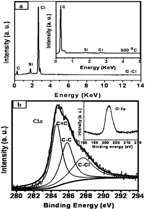Fig. 1 (a) EDAX spectrum of chlorinated graphene (G-Cl). Inset shows the EDAX spectrum after heating G-Cl at 500 °C for 4 h. (b) C 1s core level XP spectrum of G-Cl. Inset shows the Cl 2p signal in XPS.

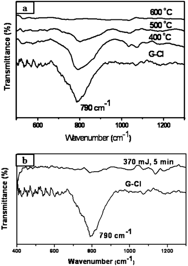Fig. 2 (a) IR spectra of G-Cl heated for 4 h at 400 °C, 500 °C and 600 °C. (b) IR spectra of G-Cl and G-Cl subjected to laser radiation (370 mJ, 5 min).

The chlorinated graphene (G-Cl) sample is stable under ambient conditions and can be stored for long periods. We have examined the thermal stability of G-Cl in detail. In Fig. 2(a), we show the infrared spectra of the chlorinated sample heated to different temperatures. We observe a decrease in C–Cl band intensity on heating progressively and it completely disappears above 500 °C. In Fig. 3 we show the loss of chlorine from the chlorinated graphene with increase in temperature. The EDAX spectrum of the sample heated to 500 °C also shows the disappearance of the chlorine signal (see inset of Fig. 1(a)). Clearly all the chlorine is eliminated on heating G-Cl to 500 °C. We could also remove chlorine in G-Cl on irradiation with a laser (Lambda physik KrF excimer laser (λ = 248 nm, τ = 30 ns, rep. rate = 5 Hz, laser energy = 370 mJ)). We show the effect of laser irradiation in Fig. 2(b) which shows the absence of the C–Cl stretching band in the infrared spectrum on irradiation for 5 min. Dechlorination by laser irradiation shows a photothermal effect. Thus, G-Cl dispersed in carbon tetrachloride shows an increase in temperature by 26 °C on irradiation. The Raman spectrum of the dechlorinated sample showed a decrease in the relative intensity of the D-band to the value in the starting graphene sample. Interestingly, the nature of graphene was not affected on chlorination and dechlorination.

Fig. 3 Loss of chlorine from chlorinated graphene with increase in temperature.

In Fig. 4 we compare the TEM images of the starting graphene sample and of the dechlorinated sample. AFM images of the two samples are also comparable. The dechlorinated samples can be chlorinated again satisfactorily.

Fig. 4 TEM images of (a) graphene and (b) dechlorinated graphene. AFM images of these samples are shown alongside.

We have also carried out bromination of graphene (see experimental section for details). Fig. 5(a) shows a typical EDAX spectrum of brominated graphene (G-Br) containing 25 wt.% (4.8 at.%). XPS analysis of the brominated sample shows Br 3d, 3p3/2 and 3p1/2 features at 70.9, 183.9 and 190.8 eV respectively as shown in Fig. 5(b) and (c).^18,19Bromine in the samples could be eliminated on heating at 500 °C as evidenced by the EDAX spectrum given in the inset of Fig. 5(a).

Fig. 5 (a) EDAX spectrum of brominated graphene (G-Br). Inset shows the EDAX spectrum after heating at 500 °C for 4 h. Core level XP spectra of G-Br show (b) Br 3d and (c) Br 3p signals.

The present study demonstrates that one can achieve chlorination of few-layer graphene at least up to 56 wt.% by UV irradiation in liquid-chlorine medium. This yield is better than from photochemical chlorination by CVD.¹⁶ It may be possible to attain higher chlorine content by other means. The chlorinated graphene consists of sp³ C–Cl bonds which are stable at room temperature. However, the chlorine can be removed on heating to around 500 °C or by laser irradiation. Clearly, dechlorination is associated with a small barrier just as the decomposition of hydrogenated graphene.⁸ The strain in the chlorinated sample appears to drive the dechlorination to form the more stable graphene. It is noteworthy that chlorination of graphene is reversible. The present study demonstrates that few-layer graphene can be used to store chlorine and bromine.

Experimental

Few-layer graphene (G) was prepared by the arc evaporation of graphite in a water-cooled stainless steel chamber filled with a mixture of hydrogen (200 torr) and helium (500 torr) without using any catalyst.²⁰ In a typical experiment, a graphite rod (Alfa Aesar with 99.999% purity, 6 mm in diameter and 50 mm long) was used as the anode and another graphite rod (13 mm in diameter and 60 mm in length) was used as the cathode. The discharge current was in the 100–150 A range, with a maximum open circuit voltage of 60 V. The graphene obtained by this method contains 2–4 layers.

Graphene (15 mg) was taken in 30 mL of carbon tetrachloride (spectroscopic grade) and sonicated for 20 min using a ultrasonicator. The suspension obtained was transferred to a 500 mL quartz vessel which was fitted with a condenser maintained at −77 °C. The reaction chamber was purged with high purity nitrogen (99.9999%) for 30 min and chlorine gas was passed through the chamber. The gaseous chlorine condensed in the quartz vessel. The quartz vessel containing around 20 mL of liquid chlorine was heated to 250 °C with simultaneous irradiation of UV light (Philips 250 Watt high pressure Hg vapor lamp) for 1.5 h. The solvent and excess chlorine was removed, leaving a transparent film on the walls of the quartz vessel. The solid was dispersed in absolute alcohol under ultrasonication, filtered and washed with distilled water and absolute alcohol. The filtrate was then re-dispersed in 40 ml of distilled water, ultrasonicated for 2 min and centrifuged. The black supernatant obtained was separated and filtered using a PVDF membrane (200 nm pore size). The yield from the 15 mg graphene sample was around 3–4 mg. In the case of bromination, 12 mg of graphene was taken in the quartz vessel, to which 20 mL of liquid bromine was added. The mixture was sonicated for 10 min using an ultrasonicator. To this 0.5 g of carbon tetrabromide was added. The quartz vessel was then heated to 250 °C with simultaneous irradiation of UV light just as in chlorination. The excess bromine was removed and the product washed with sodium thiosulfate. The solid residue was then washed with water and absolute alcohol several times to remove sodium thiosulfate and then dispersed in 40 mL distilled water and centrifuged. The black supernatant obtained was separated and filtered using a PVDF membrane (200 nm pore size). The yield from the 12 mg sample was around 2–3 mg.

The halogenated samples were characterized by EDAX, XPS, TEM, Raman spectroscopy, AFM, TGA and IR spectroscopy. They were heated to different temperatures in the 200–600 °C range and the products subjected to EDAX analysis and other methods of characterization. To study the laser induced transformation of the chlorinated graphene, the chlorinated graphene samples were first spin-coated on a NaCl crystal and dried slowly to evaporate all solvent present on the crystal. For laser irradiation, the NaCl crystal (coated with the sample) was tightly affixed (covered) with a quartz plate so that material could not get delaminated from the substrate. Lambda physik KrF excimer laser (λ = 248 nm, τ = 30 ns, rep. rate = 5 Hz) was employed for this purpose. The aluminium metal slit (beam shaper), which usually gives a rectangular beam, was removed while laser irradiation was carried out. This makes laser energy almost uniform throughout the area where the sample is present. Excimer laser beam direction was aligned normal to the substrate. A laser beam energy of 370 mJ was employed to achieve the dechlorination of graphene.

EDAX spectrum was recorded by employing FEI NOVA NANOSEM 600. X-ray photoelectron spectra were recorded with an Omicron nanotechnology spectrometer. To record the IR spectra, the chlorinated graphene samples were spin-coated on a NaCl crystal and spectra recorded using a Bruker IFS 66V/S. TGA of the samples was carried out in a flowing argon atmosphere or in air with a heating rate of 10 °C per minute using a Mettler-Toledo-TG-850 apparatus. TEM images were obtained with a JEOL JEM 3010 instrument fitted with a Gatan CCD camera operating at an accelerating voltage of 300 kV. Raman spectra were recorded at different locations of the sample using Jobin Yvon LabRam HR spectrometer with 632 nm Ar laser. AFM measurements were performed using an Innova atomic force microscope.

References

1. A. K. Geim and K. S. Novoselov, Nat. Mater., 2007, 6, 183.
2. C. N. R. Rao, A. K. Sood, K. S. Subrahmanyam and A. Govindaraj, Angew. Chem., Int. Ed., 2009, 48, 7752.
3. C. N. R. Rao and R. Voggu, Mater. Today, 2010, 13, 34.
4. X. Wang, J.-B. Xu, W. Xie and J. Du, J. Phys. Chem. C, 2011, 115, 7596.
5. P. Chaturbedy, H. S. S. R. Matte, R. Voggu, A. Govindaraj and C. N. R. Rao, J. Colloid Interface Sci., 2011, 360, 249.
6. K. S. Subrahmanyam, A. K. Manna, S. K. Pati and C. N. R. Rao, Chem. Phys. Lett., 2010, 497, 70.
7. D. C. Elias, R. R. Nair, T. M. G. Mohiuddin, S. V. Morozov, P. Blake, M. P. Halsall, A. C. Ferrari, D. W. Boukhvalov, M. I. Katsnelson, A. K. Geim and K. S. Novoselov, Science, 2009, 30, 610.
8. K. S. Subrahmanyam, P. Kumar, U. Maitra, A. Govindaraj, K. P. S. S. Hembram, U. V. Waghmare and C. N. R. Rao, Proc. Natl. Acad. Sci. U. S. A., 2011, 108, 2674.
9. S.-H. Cheng, K. Zou, F. Okino, H. R. Gutierrez, A. Gupta, N. Shen, P. C. Eklund, J. O. Sofo and J. Zhu, Phys. Rev. B, 2010, 81, 205435.
10. S. Tang and S. Zhang, J. Phys. Chem. C, 2011, 115, 16644.
11. R. R. Nair, W. C. Ren, R. Jalil, I. Riaz, V. G. Kravets, L. Britnell, P. Blake, F. Schedin, A. S. Mayorov, S. Yuan, M. I. Katsnelson, H. M. Cheng, W. Strupinski, L. G. Bulusheva, A. V. Okotrub, I. V. Grigorieva, A. N. Grigorenko, K. S. Novoselov and A. K. Geim, Small, 2010, 6, 2877.
12. M. A. Pimenta, G. Dresselhaus, M. S. Dresselhaus, L. G. Cancado, A. Jorio and R. Saito, Phys. Chem. Chem. Phys., 2007, 9, 1276.
13. A. Das, S. Pisana, B. Chakraborty, S. Piscanec, S. K. Saha, U. V. Waghmare, K. S. Novoselov, H. R. Krishnamurthy, A. K. Geim, A. C. Ferrari and A. K. Sood, Nat. Nanotechnol., 2008, 3, 210.
14. H. Yu, Z. Zhang, Z. Wang, Z. Jiang, J. Liu, L. Wang, D. Wan and T. Tang, J. Phys. Chem. C, 2010, 114, 13226.
15. E. Papirer, R. Lacroix, J.-B. Donnet, G. Nansé and P. Fioux, Carbon, 1995, 33, 63.
16. B. Li, L. Zhou, D. Wu, H. Peng, K. Yan, Y. Zhou and Z. Liu, ACS Nano, 2011, 5, 5957.
17. C. N. R. Rao, Chemical Applications of Infrared Spectroscopy, Academic Press, New York, 1963.
18. J. F. Colomer, R. Marega, H. Traboulsi, M. Meneghetti, G. Van Tendeloo and D. Bonifazi, Chem. Mater., 2009, 21, 4747.
19. J. F. Friedrich, S. Wettmarshausen, S. Hanelt, R. Mach, R. Mix, E. B. Zeynalov and A. Meyer-Plath, Carbon, 2010, 48, 3884.
20. K. S. Subrahmanyam, L. S. Panchakarla, A. Govindaraj and C. N. R. Rao, J. Phys. Chem. C, 2009, 113, 4257–4259.

---

References

- A. K. Geim and K. S. Novoselov, Nat. Mater., 2007, 6, 183 CrossRef CAS.