New tricks by very old dogs: predicting the catalytic hydrogenation of HMF derivatives using Slater-type orbitals

Abstract

We report new experimental results on the hydrogenation of 5-ethoxymethylfurfural, an important intermediate in the conversion of sugars to industrial chemicals, using eight different M/Al₂O₃ catalysts (M = Au, Cu, Ni, Ir, Pd, Pt, Rh, and Ru) under various conditions. These data are then compared with the results for 48 bimetallic supported catalysts. The results are explained using a simple and effective model, applying catalyst descriptors based on Slater type orbitals (STOs). Each metal is described using four parameters: the height of the orbital peak, the distance of the peak from the metal atom centre, the peak width at half height, and the peak skewness. Importantly, all these parameters are derived from one simple equation, so the calculation is fast and robust. We then apply these descriptors for modeling the hydrogenation data using multivariate methods. Despite the inherent complexity of the reaction network, these simple models describe the catalysts' performance well. The general application of such descriptor models to in silico design and performance prediction of solid catalysts is discussed.

---

Introduction

In the big picture of sustainable development and green chemistry, catalysis plays a key role. This is most evident in petroleum-based processes, where solid catalysts account for over 90% of all processes by volume.^1,2 In the petrochemical and bulk chemical industries catalytic processes operate continuously, and catalyst development is usually incremental yet steady. Mostly, the basic premises are determined empirically rather than heuristically, due to the heroic efforts needed for ab initio deciphering of surface-catalysed reactions. The award of the 2007 Nobel Prize in Chemistry to Gerhard Ertl, for elucidating the mechanism of ammonia synthesis, is a measure of the challenge (and the reward) of understanding one such mechanism.^3,4 Renewable feedstocks, such as vegetal biomass, present additional catalytic obstacles. Unlike crude oil, which is made up of bare hydrocarbons, biomass is already over-functionalised. It must therefore be de-functionalised (literally, κατα λυσις: broken down). But biomass feedstocks also require new types of catalysts. For example, CoMo and NiMo are typically used for catalysing crude oil hydrodesulfurisation.^5,6 But these refinery catalysts rely on sulfur-rich feedstocks, and the lower sulfur content in biomass causes their deactivation.^7,8 Such singular changes cannot be reached using incremental improvements.^9–11

Our work centres on 5-hydroxymethylfurfural (HMF) and its derivatives, particularly the stable 5-ethoxymethylfurfural 1. This compound is readily produced from cellulose and hemicellulose via C₅ sugars, such as fructose.¹² Thanks to its multi-functionality, compound 1 can react via several routes (see Scheme 1), the end products of which are all of industrial interest. Finding selective catalysts for these routes connects thus two important green chemistry principles: replacing stoichiometric reagents with catalytic ones, and moving from petroleum-based feedstocks to renewable ones.^12,13

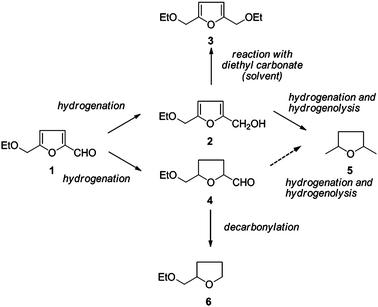Scheme 1 Reaction pathways for the hydrogenation of 5-ethoxymethylfurfural 1 indicating the major reaction products observed.

Examining the complex reaction network as shown in Scheme 1, and noting that catalytic biomass conversion may follow different paradigms than petroleum-based reactions, we decided to apply a rational approach in our catalyst search.¹⁴ In general, there are three approaches for catalyst searching: one can try and “test everything”, using high-throughput experimentation. Unfortunately, while this route has had its followers in the 1990s, scientists very quickly realized just how large a space “everything” covers.¹⁵ Alternatively, one can formulate mechanistic theories for catalytic reactions on surfaces, verifying these with kinetic experiments. However, this is costly and labour-intensive, and a wrong hypothesis may lead to a dead end. Indeed, the most effective route lies in the middle, combining catalyst screening and data-driven models with mechanistic studies (Fig. 1).^16–20

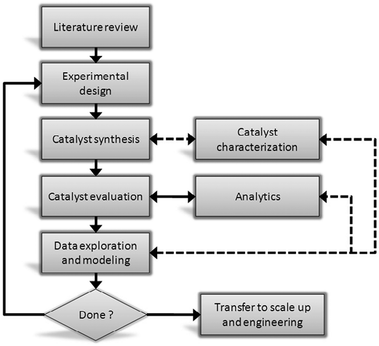Fig. 1 Workflow diagram for a model-driven catalyst development program. The solid lines indicate steps that are always required, the dotted lines indicate optional steps that may occasionally be required.

Strikingly, despite the fact that catalytic reactions on surfaces are almost insanely intricate processes, catalyst performance can be predicted well with simplified models. Here we present an approach for describing supported transition metal catalysts using only four simple descriptors, derived from the orbital functions developed by John Slater in the 1930s.²¹ We then demonstrate the models' effectiveness in predicting the performance of a large set of monometallic and bimetallic hydrogenation catalysts.

We previously reported the catalytic hydrogenation of 5-ethoxymethylfurfural 1 using bimetallic catalysts under various conditions.^12,18 Here we report new experimental results using eight monometallic catalysts M/Al₂O₃ (where M = Au, Cu, Ni, Ir, Pd, Pt, Rh or Ru; supported on alumina). Subsequently, we use this new dataset to build and validate a descriptor model for these catalysts. The model is then extended also to the bimetallic catalysts.

Experimental section

Materials and instrumentation

Quantitative gas chromatography was done using an InterScience TraceGC gas chromatograph equipped with an FID and a VF-WaxMS column (Varian #CP9205; 30 m × 0.25 mm; 0.25 μm stationary phase). The GC program consists of 3 steps: isotherm at 100 °C for 1 min; ramp at 25 °C min⁻¹ to 250 °C; and isotherm at 250 °C for 3 min. The substrate 5-ethoxymethylfurfural 1 elutes at 3.1 min and the desired product 5-ethoxymethylfurfuryl alcohol 2 at 3.5 min. Identification of unknowns was performed with a Varian GC/MS using the same column and program as above. Spectra were obtained in EI or CI modes. All chemicals were purchased from commercial sources and used as received. Precursors for the metals and their sources are given in Table 1.

Table 1 Precursors used in the catalyst synthesis

Metal	Precursor	Supplier
Au	HAuCl4·3H2O	Alfa Aesar
Cu	Cu(NO3)2·6H2O	Alfa Aesar
Ir	Ir(OAc)·H2O	Heraeus
Ni	Ni(NO3)2·6H2O	Alfa Aesar
Pd	Pd(NO3)2 aq. soln	Sigma-Aldrich
Pt	(NH3)4Pt(NO3)2	Sigma-Aldrich
Rh	Rh(NO3)3 aq. soln	Alfa Aesar
Ru	Ru(NO)(NO3)3	Sigma-Aldrich

---

Hydrogenation experiments were run using a 16-parallel Flowrence flow reactor (www.flowrence.com), using 16 quartz reactor tubes of 2 mm inner diameter. Using a capillary feed distribution system, a total liquid flow of 400 L min⁻¹ and a total gas flow of 25 N mL min⁻¹ H₂ was distributed over the reactors at a constant pressure of 25 bar. The catalyst bed volume was 200 L in all cases, using 50 mg of catalyst diluted to volume with low-surface-area silica–zirconia as an inert filler. The liquid feed contained 1 wt% of the starting material 1 dissolved in diethyl carbonate (ACS purity reagent).

General procedure for catalyst synthesis

The catalysts were prepared following a modification of a previously published procedure.¹² This uniform method was chosen to facilitate modeling only the metals' properties, without adding complexity due to varying synthesis methods. We synthesized eight monometallic catalysts (M1–M8, see Table 2) on γ-alumina (surface area of 289 m² g⁻¹, pre-dried at 105 °C). Nitrate salts were used as precursors, except for gold (chloride) and iridium (acetate), see Table 1. All catalysts had a metal loading of 1 wt% relative to the support and were prepared by wet impregnation in water (18 h impregnation at ambient temperature). After decanting the excess liquid, the catalysts were dried in air at 105 °C for 18 h, followed by calcination in air at 320 °C for 4 h. Selected catalysts were characterized using X-ray diffraction measurements using a Bruker instrument equipped with a CuK source.¹² However, due to the small metal particle size and low overall metal loading no significant data could be obtained, so these XRD experiments were discontinued.

Table 2 Conversion and selectivity data obtained for the monometallic catalysts

Entry	Catalyst/metal^a	T ^b	Conversion (%)	Selectivity (%)
		(°C)	1	2	3	4	5	6
a All catalysts contain 1 wt% of metal on γ-Al2O3. b Catalysts were tested in a fixed bed reactor using a feed of 1 wt% 5-ethoxymethylfurfural 2 in diethyl carbonate.
1	M1/Au	80	38	29	19	—	22	4
2		100	53	17	26	—	19	5
3		120	82	7	49	—	22	5
4	M2/Cu	80	36	20	3	—	1	—
5		100	44	14	14	—	5	—
6		120	57	8	29	—	18	1
7	M3/Ir	80	95	71	4	—	12	1
8		100	72	25	24	—	18	2
9		120	79	8	53	—	22	4
10	M4/Ni	80	54	18	5	—	1	—
11		100	47	18	19	—	5	—
12		120	54	13	39	—	19	1
13	M5/Pd	80	100	—	—	78	8	—
14		100	100	20	—	32	20	29
15		120	100	11	1	18	28	35
16	M6/Pt	80	87	69	3	2	13	2
17		100	78	28	26	—	20	3
18		120	98	3	66	—	28	6
19	M7/Rh	80	68	75	3	10	12	3
20		100	67	27	20	1	18	6
21		120	94	4	54	—	24	10
22	M8/Ru	80	44	34	5	—	18	—
23		100	47	24	17	—	16	—
24		120	68	12	37	—	19	1

---

Example: Pt on alumina (M6). A stock solution of tetraaminoplatinum(II) nitrate was prepared by dissolving 3.1 grams of (NH₃)₄Pt(NO₃)₂ in 25 mL demineralized water. To one gram of pre-dried Al₂O₃ (surface area 289 m² g⁻¹) support (overnight at 105 °C in air), 160 μL of Pt-stock solution was added, after which the total volume of the system was adjusted to 2.0 mL. The resulting slurry was homogenized for 24 h under ambient conditions. Then, the homogenized sample was dried at 105 °C for 18 h and then calcined in air at 320 °C for 4 h (with ramp rates of 5 °C min⁻¹ for both the drying and the calcination). Prior to reaction, each catalyst was reduced for 2 h in the catalyst test reactor using 6 bar of 5% H₂ in N₂ at 300 °C.

Procedure for catalytic hydrogenation experiments

Catalyst testing was performed in a continuous 16-parallel fixed bed reactor as described above using diethyl carbonate as a solvent. All catalysts were tested at 80 °C, 100 °C and 120 °C. Liquid samples were collected at the reactor exit and analyzed by GC-FID. To obtain a consistent data set, the same conditions were used for all catalysts, regardless of their intrinsic activity. Due to the small amount of catalyst used, and the fact that the catalyst was diluted with inert material, recovery of the spent catalyst after reaction for further characterization was not possible.

Results and discussion

In general, catalysts M1–M8 give a simpler product mixture (see Scheme 1) than the bimetallic ones reported earlier.¹² The predominant reaction is the reduction of the carbonyl bond, giving the unsaturated alcohol 2. From there either etherification to the diether 3 occurs, or combined hydrogenation and hydrogenolysis to dimethyltetrahydrofuran 5. The Pd catalyst M5 follows a different pathway, where the furan ring is reduced preferentially, yielding the saturated aldehyde 4. This aldehyde also undergoes further reduction and hydrogenolysis to yield dimethyltetrahydrofuran 5. Alternatively, the saturated aldehyde 4 can undergo decarboxylation, yielding the monosubstituted tetrahydrofuran 6. This last reaction is most pronounced with the Pd catalyst, due to the formation of a large fraction of 4. Table 2 gives the reaction conditions and product yields. In principle, all products in Scheme 1 are of interest in various applications. The mass balance is 70–90% when taking into account the yields of products 2–6. By-products closing the mass balance are dimethylfuran, various hydrogenolysis products where the C–O bond in the ethoxy substituent is cleaved, and oligomers (mostly dimers and trimers) in varying amounts. Typically, when conversion is low, so is the selectivity to products 2–6. The decrease or stagnation in conversion when moving from 80 °C to 100 °C can be attributed to product inhibition. When the temperature is further increased to 120 °C conversion typically increases again, apparently overcoming desorption limitations. Generally speaking, the products observed are in line with those observed in the hydrogenation of other unsaturated aldehydes,²²e.g. crotonaldehyde^23,24 and cinnamaldehyde.^25,26 More details on the possible mechanism of these reactions are reported elsewhere.¹²

Applying Slater-type orbitals (STOs) as catalyst descriptors

Heterogeneous catalysis is essentially an electronic interaction between molecules and a metal, wherein chemical reactions are initiated by charge donations to and from the metal.^27–30 Thus, the distribution of electrons in a metal and the shape of the orbitals relate directly to its catalytic performance. More specifically, we are interested in the number of available electrons and their location relative to the atomic center and relative to each other. Slater-type orbitals (STOs) capture these parameters nicely. Since their introduction in 1930,²¹ STOs have been used extensively in theoretical and computational chemistry.^31–34 Essentially, the original form of the equation devised by John Slater remained intact throughout the years. Here we are interested only in the radial part of the STO, described as:

R(r) = Nrⁿ⁻¹e^−ζr (1)

where , r represents the distance from the atomic core, Z the nuclear charge, σ the shielding constant, and n* the effective quantum number n (all in atomic units). The normalization constant N is obtained by integrating eqn (1), such that the total integral accounts for one electron.

Using eqn (1) and the parameters determined by Herman³⁵ for the valence electrons, we calculated the STOs for the metals M1–M8. Fig. 3 shows the STOs for Ni and Pt. The peak maximum is located further away from the core for the higher orbital indices. In the summed profiles, we summed the STOs according to the number of electrons per angular momentum. For transition metals, the (n − 1) d-orbital has a large impact on the overall shape of the curve. To use these STOs as descriptors, we assigned them four straightforward parameters: The peak position, apex height, width at half height, and skewness (see Fig. 2). This is preferred over a large vector of binned R(r) values per catalyst, as it avoids overfitting.

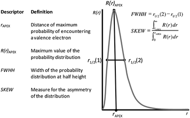Fig. 2 Definition and graphical explanation of the four peak parameters used as descriptors. The parameters used to calculate the orbital functions for the metals studied here are given in Table 3.

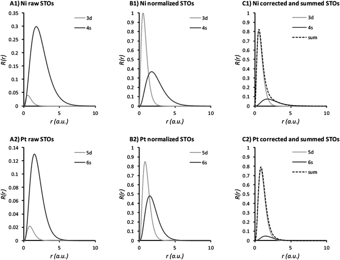Fig. 3 Slater-type orbitals for the valence electrons Ni and Pt. The first row of plots is associated with Ni, the second row of plots is associated with Pt. The panels denoted A1 and A2 give the raw profiles of the individual valence orbitals, the panels denoted B1 and B2 give the same profiles scaled to unit area and the panels denoted C1 and C2 give the profiles scaled to the amount of electrons present (solid lines) and the final summation used to derive the descriptor values from (dotted line).

Table 3 Values of the parameters used to calculate the STOs for each of the elements used²⁹

Metal	Orbital	Occupation	ζ	n*^a
a The effective quantum number (n*) is used instead of the quantum number n to prevent underestimation of the lower orbitals in large atoms. For n ∈ {1, 2, 3} the effective quantum number is equal to n. For larger values of n, a lower value of n* is used (n = 4 → n* = 3.7; n = 5 → n* = 4.2; n = 6 → n* = 4.35).^21
Main metals
Au	6s	1	2.3185	4.35
	5d	10	4.0525	4.2
Cu	4s	1	1.5791	3.7
	3d	10	3.8962	3
Ir	6s	2	2.2167	4.35
	5d	7	3.7077	4.2
Ni	4s	2	1.5532	3.7
	3d	8	3.7017	3
Rh	5s	1	1.7671	4.2
	4d	8	3.3113	3.7
Ru	5s	1	1.7347	4.2
	4d	7	3.1524	3.7
Pd	4d	10	3.0858	3.7
Pt	6s	1	2.2646	4.35
	5d	9	3.8996	4.2
Promoters
Bi	6s	2	2.7869	4.35
	6p	3	2.2146	4.35
Cr	4s	1	1.3804	3.7
	3d	5	2.9775	3
Fe	4s	2	1.5465	3.7
	3d	6	3.4537	3
Na	3s	1	0.8675	3
Sn	5s	2	2.4041	4.2
	5p	2	1.9128	4.2
W	6s	2	2.0190	4.35
	5d	4	3.1936	4.2

---

Modeling the monometallic catalysts data set. To test the performance of the STO descriptors in the modeling of the hydrogenation data, we constructed an Orthogonal Partial Least Squares (OPLS) model.³⁶ This model has five independent variables: the four peak parameters (r_APEX, R(r)_APEX, FWHH and SKEW) and the reaction temperature. Since the relationship between variables and responses is non-linear, cross-terms and quadratic terms are also included in the initial variable space. After constructing the initial model, the variable space is reduced. This is done by stepwise elimination of redundant variables and higher order terms. The final reduced model is obtained when a plateau in RMSEE (root mean squared error of estimate) is reached.

Note that the model hierarchy is maintained in all cases (i.e. if the model indicates that the square of temperature is a significant influence but temperature as such is not, both terms are still included in the model). The yields of the main reaction products 2, 3, 5 and 6 are used as responses (so-called dependent variables). The reasons for excluding data for the Pd catalyst and the yield of 4 are twofold. On one hand, Pd clearly shows a different reactivity compared to the other catalysts since it prefers to reduce the furan ring. Because in this aspect it is unique amongst the tested catalysts it is considered to be an outlier. This identification is in fact quite helpful – using the obtained model to predict Pd performance will result in the conclusion that Pd does not fit well to a model describing carbonyl hydrogenation. On the other hand, the yield of 4 has a non-zero response only in 5 out of the 24 cases, so no proper model can be made based on that. Since our objective was to investigate the carbonyl reduction, we did not search for more catalysts showing preference for ring hydrogenation. Further details on the statistics behind this exclusion are given in the ESI.† Using these model equations, the data from Table 2 can be calculated and compared to the original experimental data. The classical observed versus predicted plot (parity plot) is difficult to interpret in the case of multiple responses. Instead, we used a color matrix, comparing all responses simultaneously in addition to the parity plot (Fig. 4).

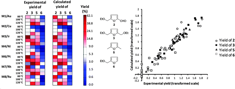Fig. 4 Matrix plot comparing observed yields (left) to the yields predicted by the OPLS model (right). The products are grouped in columns, the catalysts and temperatures are grouped in rows. The yields are coded from blue (low yield) to red (high yield). Both predicted and observed yields are plotted on the same scale. On the right hand side a parity plot representing the same information is given to facilitate interpretation. The combined model has an R² of 0.85 and a Q² of 0.76. The R² values for the individual yields are 0.75, 0.96, 0.96 and 0.74.

In general, the observed and calculated yields are in good agreement. The largest discrepancies are found in the yields of the unsaturated alcohol 2 and the diether 3. This is caused by the chemistry, rather than by the models. The diether 3 forms in a side reaction of 2 with the solvent (diethyl carbonate). This reaction becomes more pronounced as the temperature increases and is less influenced by the catalyst. Note that this reaction is not part of the reaction network associated with hydrogenation. Rather, it is a side reaction proceeding through an alternative pathway. This behavior is not fully captured by the yield, because the yield combines selectivity and activity. However, modeling yield to the diether 3 separately does give a good model (Fig. 5). The two outlying predictions (Pt and Rh at 120 °C) reflect a lack of data points on the high end of the scale.

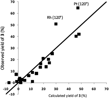Fig. 5 Parity plot for the model for the yield of the diether 3. The horizontal axis denotes the yield calculated by the model, the vertical axis denotes the experimentally observed yield. Both yields are in percent. The R² of the model is 0.80 and the RMSEE is 7.5% (leaving out the two outliers gives an R² of 0.91 and an RMSEE of 5.1%).

The data set used is rather small. Increasing it, however, is complicated by the fact that only a limited number of metals have sufficient hydrogenation activity. In this case, simply adding more metals to the data set scope would typically increase the number of poorly performing catalysts. This would bias the data set (and any model thereof) towards poor performance. Due to the small size of the data set a partitioning in training and validation set is problematic. Instead, we opted for a modification of the leave-one-out method. In each validation round, the three data points for a single metal were excluded and the model identified for the full set was refitted (see ESI† for details). This method gives more insight into the model's performance than random exclusion or measuring Q² in the case of a small data set.

By comparing the magnitude and direction of the model coefficients obtained for each validation model, one can assess the validity and the robustness of the original model. Fig. 6 shows the scaled coefficients for the validation models. Clearly, temperature is an important parameter (i.e. it has a large positive coefficient). Indeed, one would expect the response yield to increase with temperature. Regarding the peak parameters, we see that both the distance of the apex from the atom center and its magnitude increase the obtained yield of 3. This means that large atoms with many valence electrons are good candidates for catalysing the reduction of the carbonyl group. Actually, the square of the r_APEX parameter has a negative coefficient, which means there is a volcano-like optimum for the size of the atom. The width of the distribution and its skewness have a negative impact on the yield. Rationalizing this into requirements for metals, good catalyst candidates have a narrow distribution. That being said, we are less interested in the exact interpretation of the parameters, and more in the finding that there is a solid mathematical relationship between a metal's STOs and its catalytic performance. This means that for a more complicated case, for example using bimetallic catalysts, one can screen potentially interesting materials in silico. Such a directed search method is preferred over the “test everything” approach.

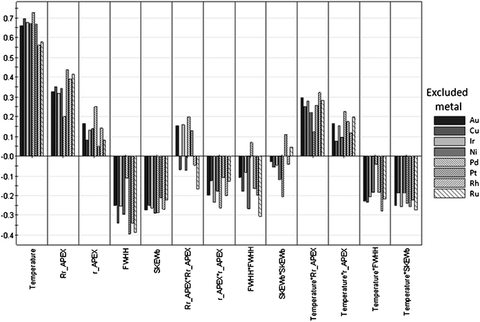Fig. 6 Scaled model coefficients for the validation models for the combined reduction and etherification to 3 by monometallic catalysts. The direction of the bars relative to the horizontal axis indicates the sign of each model coefficient. The starting point for these validation models is the monometallics model described in Fig. 4.

A more complex case – bimetallic catalysts. The results using monometallic catalysts show the applicability of our descriptors. However, real-life catalysts are typically more complex. To demonstrate that the peak parameters of the STOs also work in complex cases, we tested their performance of a set of bimetallic catalysts. Here each catalyst consists of 1 wt% loading of a main metal, plus a fixed loading of a promoter metal (10 mol% relative to the main metal). The main metals (Au, Cu, Ni, Ir, Pd, Pt, Rh and Ru) were the same as those in catalysts M1–M8. The promoters (Bi, Cr, Fe, Na, Sn and W) were selected for their diversity. The experimental details of the synthesis and characterization of these bimetallic catalysts are published elsewhere.^13,18 To simplify the modeling results presented here we focus on one of the observed reaction pathways only, the hydrogenation of the carbonyl group, resulting in the unsaturated alcohol 2, followed by etherification resulting in the diether 3. As in the monometallic case presented before, the other pathways can be explained as well.

As the loading of the main metal and the main metal : promoter ratio are consistent throughout the data set, the descriptors can be treated separately. This means that we use one set of peak parameters for the main metals, and another for the promoter metals. Table 4 gives the peak parameters calculated for all main metals and promoters. In cases where different ratios are used, a linear combination of the atomic orbitals could be used, giving a single set of peak parameters (alternatively, one can compare the distances between the peaks of two metals in a bimetallic system). Using a linear combination of atomic orbitals gives the possibility of comparing systems with different numbers of metals.

Table 4 Calculated peak attributes for the eight main metals and six promoters^a

Metal	r APEX	R(r)APEX	FWHH	SKEW
a A worked example for Au using eqn (1) and the parameters in Table 3: calculate the distribution for the 6s orbital using ζ = 2.3185 and n* = 4.35 over the interval 0 to 10 atomic units at an appropriately small spacing. Normalize the distribution to an area corresponding to 1 electron. Then calculate the distribution for the 5d orbital using ζ = 4.0525 and n* = 4.2 over the interval 0 to 10 atomic units at the same spacing as used for the 6s orbital. Normalize this distribution to an area corresponding to 10 electrons. To obtain the summed RDF, simply add the two distributions obtained for the separate orbitals. Finally, the summed orbitals need to be normalized again to an area of one to compare elements containing different amounts of valence electrons at the same scale. This is of particular importance for the magnitude of the peak apex.
Main metals
Au	0.802	0.828	1.091	1.923
Cu	0.518	0.967	0.893	2.334
Ir	0.905	0.696	1.274	2.058
Ni	0.553	0.822	0.984	2.668
Pd	0.875	0.727	1.272	1.894
Pt	0.836	0.793	1.139	1.925
Rh	0.830	0.713	1.241	2.100
Ru	0.876	0.672	1.314	2.108
Promoters
Bi	1.354	0.508	1.813	1.847
Cr	0.688	0.690	1.216	2.513
Fe	0.601	0.730	1.094	2.790
Na	2.305	0.237	3.913	2.069
Sn	1.463	0.460	2.001	1.873
W	1.089	0.568	1.570	2.099

---

We then built an OPLS model, using all the points in the data set with a conversion exceeding 5%. This time, there are enough data for a split into a training (n = 81) and a validation set (n = 42). The observed versus predicted plot in Fig. 7 shows the model's performance for the combined yield of unsaturated alcohol 2 and the diether 3. This captures the total amount of carbonyl reduction products in a single response. It shows a wide range of observed values, which is good for modeling purposes. Other responses (conversion, yields, selectivities, or rates) can be modeled as well. For the sake of demonstration we limit ourselves here to the main products 2 and 3. Overall, the model describes well the effects of both temperature and catalyst composition. From the experimental data we already learned that temperature is the dominant parameter in the etherification of 2 to the diether 3. At higher temperatures, most of 2 converts to 3.

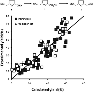Fig. 7 Observed vs. predicted plot for 48 bimetallic catalysts tested at 3 temperatures for the combined yield of 2 and 3. The horizontal axis shows the predicted yields by our model, the vertical axis shows the experimentally obtained yield. The quality of the model is as follows: training set, R² = 0.83; RMSEE = 3.7 and prediction set, Q² = 0.79; RMSEP = 9.1.

To evaluate the performance of the descriptors in the absence of temperature effects, we also used a model of only STO descriptors to describe the hydrogenation of 1 to 2. This model was trained using only the data obtained for bimetallic catalysts at a test temperature of 80 °C. The data set, 39 points with a conversion >5%, was partitioned in a training set of 26 points and a test set of 13 points by means of random exclusion. Fig. 8 compares the experimental values with the predicted ones. The model's performance is excellent, demonstrating the power of the STO descriptors for explaining the performance of bimetallic catalysts. Comparing the results of the two previous models (Fig. 4 and 7) with the results of the isothermal model in Fig. 8 shows a strong improvement in terms of model quality of the latter. This is explained by the fact that at 80 °C the observed reaction network is more simple in nature. The largest contributor to this is the fact that the further reaction of the unsaturated alcohol 2 with the ether 3 is not significant at this low temperature, which means hydrogenation performance can be expressed using just the yield of 2 as a measure. At higher temperatures the hydrogenation performance can only be measured by taking the combined yield of 2 and 3 into consideration.

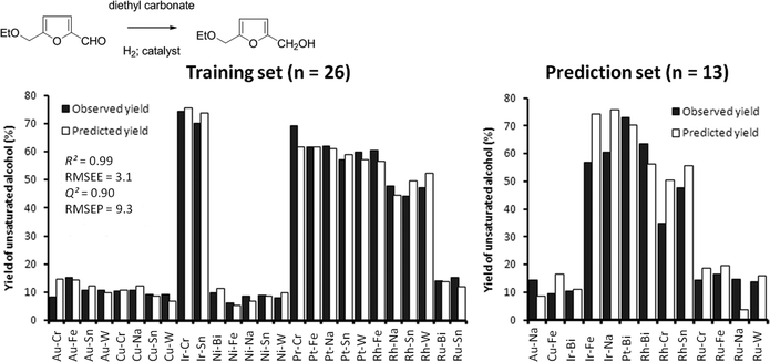Fig. 8 Performance of the training and prediction set for the model describing the conversion to the unsaturated alcohol 2. The solid bars denote the experimentally observed yield of 2. The open bars denote yield as predicted (calculated) by the model. The prediction set has been randomly selected.

For both the monometallic and bimetallic catalysts used we focus on using calculated descriptors rather than descriptors derived from characterization. This is due to the relatively large number of catalysts used and the cost, in time and effort, associated with the characterization of these materials. As such, this is one of the imposed limitations of using parallel reactor technology. Although we use a consistent catalyst synthesis method throughout the data set, modest differences in metal particle size and degree of reduction can occur. The fact that our models work supports the hypothesis that the catalysts are quite similar in these attributes. That said, one must assess the need for further characterization of key catalysts on a case by case basis. This means that when developing catalysts using parallel reactor equipment, occasional side-steps to larger scale equipment using larger catalyst amounts will be required.

The specific models described here pertain to a particular reaction, catalyst support and catalyst synthesis method. Nevertheless, the method is generic. One can apply it to other systems, provided that one collects the pertinent experimental data. For example, to include the support as an integral part of the model, a variety of supports must be tested. In addition, relevant descriptors for these supports would need to be identified. Nor is one limited to a single class of descriptors. The more relevant descriptors are included upfront, the more robust the model will be. Once the experimental data are evaluated, irrelevant descriptors are discarded.²⁰

The data and modeling thereof presented here were generated for the purpose of demonstrating the method. Considering the limited scope of available metals for this type of selective hydrogenation leaves little room for predicting a better catalyst. That said, if one removes either Pt or Ir from the model training set and then predicts the performance using the resulting model, these metals will be identified as high-selectivity candidates. This implies that our method is truly predictive, and thus useful for searching of novel catalysts.

Conclusions

Simple parameters derived from Slater-type orbitals can be used as powerful descriptors in heterogeneous catalysis. These descriptors explain well monometallic and bimetallic catalyst performance in the hydrogenation of 5-ethoxymethylfurfural. The fact that the computational cost of such descriptors is practically zero makes them attractive for virtual screening applications. Thus, at the start of a project, one can select an initial set of diverse catalysts based on their descriptor values and screen in silico large sections of the catalyst space (in this case, bimetallic catalysts containing a main metal and a promoter metal). The model can then be used for indicating regions where good catalysts are likely to be found. In practice, the accuracy of the numerical prediction of the figures of merit is of little interest. The key value of these models is in steering next generations of experiments such that after each iteration the data set becomes more biased towards, for example, high conversion and/or selectivity.³⁷

Definitions

Training set	Subset of the data set that is used to construct a model.
Validation or prediction set	Subset of the data that is not used to construct the model but is used as an unseen test set to assess model performance.
R ^2	Squared correlation coefficient between the observed values and the values calculated by the model for the training set.
Q ^2	Squared correlation coefficient between the observed values and the values predicted by the model for the validation set.
RMSEE	Root mean square error of estimate for the observations in the training set.
RMSEP	Root mean square error of estimate for the observations in the validation set.

Acknowledgements

We thank the Netherlands Organization for Scientific Research (NWO) for funding received under the Casimir program, and the Netherlands Research School Combination-Catalysis (NRSC-C) for a fundamental research project grant.

Notes and references

1. R. A. Sheldon and H. van Bekkum, Fine chemicals through heterogeneous catalysis, Wiley-VCH, 2001.
2. J. M. Thomas and W. J. Thomas, Principles and practice of heterogeneous catalysis, Wiley-VCH, 1997.
3. G. Ertl, Angew. Chem., Int. Ed., 2008, 47, 3524–3535.
4. J. H. Sinfelt, Surf. Sci., 2002, 500, 923–946.
5. E. Lecrenay, K. Sakanishi, I. Mochida and T. Suzuka, Appl. Catal., A, 1998, 175, 237–243.
6. J. Ramirez, R. Contreras, P. Castillo, T. Klimova, R. Zárate and R. Luna, Appl. Catal., A, 2000, 197, 69–78.
7. S. Czernik and A. V. Bridgwater, Energy Fuels, 2004, 18, 590–598.
8. Y. C. Lin and G. W. Huber, Energy Environ. Sci., 2009, 2, 68–80.
9. T. F. Degnan Jr, Stud. Surf. Sci. Catal., 2007, 170, 54–65.
10. S. B. T. Nguyen and T. M. Trnka, The Discovery and Development of Well Defined, Ruthenium Based Olefin Metathesis Catalysts, Wiley-VCH, 2003.
11. P. Strasser, J. Comb. Chem., 2008, 10, 216–224.
12. E. J. Ras, S. Maisuls, P. Haesakkers, G. J. Gruter and G. Rothenberg, Adv. Synth. Catal., 2009, 351, 3175–3185.
13. T. Werpy and G. Petersen, Top value added chemicals from biomass, vol. I, US-DOE, 2004.
14. Z. Strassberger, M. Mooijman, E. Ruijter, A. H. Alberts, A. G. Maldonado, R. V. A. Orru and G. Rothenberg, Adv. Synth. Catal., 2010, 352, 2201–2210.
15. E. Burello, D. Farrusseng and G. Rothenberg, Adv. Synth. Catal., 2004, 346, 1844–1853.
16. B. K. Alsberg, V. R. Jensen and K. J. Børve, J. Comput. Chem., 1996, 17, 1197–1216.
17. E. Burello and G. Rothenberg, Adv. Synth. Catal., 2005, 347, 1969–1977.
18. E. J. Ras, B. McKay and G. Rothenberg, Top. Catal., 2010, 53, 1202–1208.
19. C. Klanner, D. Farrusseng, L. Baumes, M. Lengliz, C. Mirodatos and F. Schuth, Angew. Chem., Int. Ed., 2004, 43, 5347–5349.
20. A. G. Maldonado and G. Rothenberg, Chem. Soc. Rev., 2010, 39, 1891–1902.
21. J. C. Slater, Phys. Rev., 1930, 36, 57–64.
22. P. Gallezot and D. Richard, Catal. Rev. Sci. Eng., 1998, 40, 81–126.
23. M. A. Vannice and B. Sen, J. Catal., 1989, 115, 65–78.
24. M. Englisch, V. S. Ranade and J. A. Lercher, Appl. Catal., A, 1997, 163, 111–122.
25. J. P. Breen, R. Burch, J. Gomez-Lopez, K. Griffin and M. Hayes, Appl. Catal., A, 2004, 268, 267–274.
26. A. B. Da Silva, E. Jordao, M. J. Mendes and P. Fouilloux, Appl. Catal., A, 1997, 148, 253–264.
27. T. Bligaard, M. P. Andersson, K. W. Jacobsen, H. L. Skriver, C. H. Christensen and J. K. Norskov, MRS Bull., 2006, 31, 986–990.
28. T. Bligaard, J. K. Norskov, S. Dahl, J. Matthiesen, C. H. Christensen and J. Sehested, J. Catal., 2004, 224, 206–217.
29. S. Dahl, A. Logadottir, C. J. H. Jacobsen and J. K. Norskov, Appl. Catal., A, 2001, 222, 19–29.
30. M. Mavrikakis, J. K. Norskov, AIChE Proceedings, 2001.
31. F. E. Harris and H. H. Michels, J. Chem. Phys., 1965, 43, S165–S169.
32. W. J. Hehre, R. F. Stewart and J. A. Pople, J. Chem. Phys., 1969, 51, 2657–2664.
33. I. I. Guseinov, J. Phys. B: At. Mol. Phys., 1970, 3, 1399–1412.
34. J. W. Davenport, Phys. Rev. B, 1984, 29, 2896–2904.
35. A. Herman, Modell. Simul. Mater. Sci. Eng., 2004, 12, 21–32.
36. J. Trygg and S. Wold, J. Chemom., 2002, 16, 119–128.
37. Note that the present test case demonstrates the capabilities of the method using data available in the public domain. As this research is part of a public–private initiative (CASIMIR), Avantium has also successfully applied this methodology to proprietary data sets, including the selective oxidation of alkanes and the hydrogenolysis of biomass derived feedstocks.

---

Footnote

† Electronic supplementary information (ESI) available: A detailed description of the modeling methods, a description of the subsets data selection process, details of the data and methods used in the model validation process, a typical example of the model equations and their application, and seven additional references. See DOI: 10.1039/c2cy20193c

---