The mathematical origins of the kinetic compensation effect: 2. the effect of systematic errors
Received
19th August 2011
, Accepted 25th October 2011
First published on 14th November 2011
Abstract
The kinetic compensation effect states that there is a linear relationship between Arrhenius parameters ln A and E for a family of related processes. It is a widely observed phenomenon in many areas of science, notably heterogeneous catalysis. This paper explores mathematical, rather than physicochemical, explanations for the compensation effect in certain situations. Three different topics are covered theoretically and illustrated by examples. Firstly, the effect of systematic errors in experimental kinetic data is explored, and it is shown that these create apparent compensation effects. Secondly, analysis of kinetic data when the Arrhenius parameters depend on another parameter is examined. In the case of temperature programmed desorption (TPD) experiments when the activation energy depends on surface coverage, it is shown that a common analysis method induces a systematic error, causing an apparent compensation effect. Thirdly, the effect of analysing the temperature dependence of an overall rate of reaction, rather than a rate constant, is investigated. It is shown that this can create an apparent compensation effect, but only under some conditions. This result is illustrated by a case study for a unimolecular reaction on a catalyst surface. Overall, the work highlights the fact that, whenever a kinetic compensation effect is observed experimentally, the possibility of it having a mathematical origin should be carefully considered before any physicochemical conclusions are drawn.
Introduction
The temperature dependence of the rates of many chemical processes are normally described well by the Arrhenius equation. This specifies that the rate constant for the process obeys:| | 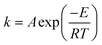 | (1) |
where E is the activation energy, A is the pre-exponential factor, R is the universal gas constant, and T is absolute temperature. Values of the Arrhenius parameters are normally obtained from a so-called Arrhenius plot in which experimental ln k values are plotted against 1/T. The kinetic compensation effect is said to occur when there is a linear relationship between ln A and E for a family of related chemical processes.1 A plot of ln A against E is sometimes referred to as a Constable plot after its first proponent.2 The kinetic compensation effect is a widely observed phenomenon in many areas of science, notably heterogeneous catalysis3–6 but also a wide variety of other areas of chemistry.7,8 However, its origins remain the subject of debate in the scientific literature, as discussed in the comprehensive review of Liu and Guo in 2001.1
The main reason for the confusion in the literature is that there are a variety of different manifestations and different reasons for the compensation effect. For some experiments, a kinetic compensation effect can arise for purely mathematical reasons as will be discussed in this work and the accompanying paper.9 In other experiments, the compensation effect may have an underlying physical significance. A wide variety of physical reasons for the kinetic compensation effect have been proposed in the literature for particular situations. However, some of the explanations for observed compensation effects have overlooked the possibility of a purely mathematical origin for that particular case.
The aim of this work and the accompanying paper9 is to explain the possible mathematical origins of the compensation effect. While some of these explanations have been previously described in the literature, research papers continue to be published that do not take them into account. This work extends previous explanations and illustrates them with examples. In this way, it is hoped to dispel the controversy and arguments in the literature on the kinetic compensation effect. Physicochemical explanations for the compensation effect will only need to be sought in those cases when the compensation effect is not arising from a mathematical origin.
In the accompanying paper,9 the effect of random errors in kinetic measurements is discussed. It is proven that random experimental errors can create an apparent compensation effect, sometimes termed the statistical compensation effect, even for a family of samples with identical values of Arrhenius parameters.
This paper is concerned with systematic errors. These may be in the experimental values of kinetic parameters that are used to determine Arrhenius parameters. In the first part of this paper, it will be shown, both theoretically and by numerical simulations, that systematic errors of this type can create an apparent compensation effect. Another class of systematic error can arise in the special case when the Arrhenius parameters are functions of another parameter. An example of this situation comes when analysing the results of temperature programmed desorption (TPD) experiments when the activation energy for desorption is a function of coverage. This will be discussed in the second part of this paper. It will be shown, both theoretically and by numerical simulations, that a common method for analysing TPD data creates an apparent compensation effect even when the experimental data is from errors. In the third part of this paper, the effect of analysing the overall rate of reaction, rather than a rate constant, is investigated. It will be shown that this can create an apparent compensation effect, but only under some conditions. To illustrate this result, an example case study for a unimolecular reaction on a catalyst surface will be presented.
1. The effect of systematic errors in kinetic measurements
When there are systematic errors in the measurement of rate constants, the values of Arrhenius parameters obtained from the analysis will not equal the actual values. The values of measured activation energy Emeas and measured pre-exponential factor Ameas are defined to obey:| | 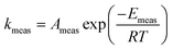 | (2) |
Values for measured Arrhenius parameters are normally found from a graph of ln kmeas against 1/T, with the gradient providing (−Emeas/R) and the intercept on the y-axis providing ln Ameas. Equivalently, the measured activation energy can be defined to be:| | 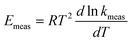 | (3) |
while the measured pre-exponential factor will obey:| |  | (4) |
or equivalently:| | 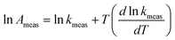 | (5) |
In this section, we shall examine the influence that different forms of systematic error in the measurement of rate constant k have on the determined values of ln Ameas and Emeas.
1.1 A systematic error that is constant
Consider the case that the true Arrhenius parameters ln A and E are constant for a sample, but there is a systematic error in the measurement of rate constant k. Assume initially that the systematic error is a constant ε that is independent of temperature or any other parameter. In this case, the measured value of rate constant is:where k is the true rate constant that obeys eqn (1). The measured activation energy can be found by putting eqn (6) into eqn (3). Algebra shows that:| |  | (7) |
Similarly the measured pre-exponential factor can be found from eqn (4) and will be:| |  | (8) |
Even though the true Arrhenius parameters are constant, the values of ln Ameas and Emeas will depend slightly on temperature in this case. In particular, Emeas will differ from the true value of the activation energy, with the difference being greatest at lower temperatures (when k is small).
If values of ln Ameas and Emeas are obtained at different temperatures and plotted on a Constable plot, then the slope will be:
| |  | (9) |
Putting
eqn (7) and (8) into
eqn (9), gives:
| |  | (10) |
Over the temperature range of most kinetic measurements, 1/
RT does not vary much and so the slope on the Constable plot will be roughly constant. This means that a reaction with fixed values of ln
A and
E will show an apparent compensation effect when there is a constant systematic error in the measurement of the rate constant
k.
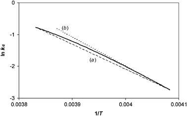
This result is illustrated in Fig. 1. Here numerical simulations were performed for a chemical reaction with a fixed value of ln A and a fixed value of E over the temperature range 300–350 K. A constant systematic error in k was added to the data—this error was taken to be half the magnitude of the rate at the lowest temperature. The simulated data were plotted on an Arrhenius plot, which enables Arrhenius parameters to be measured at each temperature. These parameters were then plotted on a Constable plot as shown in Fig. 1(b). It can be seen that the resulting values of Emeas are less than the true value (50 kJ/mol in this example) in agreement with eqn (7). The value of the gradient agrees with the prediction of eqn (10), being 1/RT which varies slightly from point to point. However, the variation is small—the curve is very close to a straight line. The systematic error has therefore created an apparent compensation effect, with the gradient of the plot being 1/RTave where Tave is a weighted average of the temperatures used in the kinetic study.
 |
| | Fig. 1 (a) An Arrhenius plot showing data points generated in the temperature range 300–350 K using a constant value of ln A (= 20) and E (= 50 kJ/mol), but with a constant error in measured k value of 0.5 time−1. Because of the systematic error, the trend line (shown by the dashes) is not exactly straight. As a result, the gradient of the tangent to the trend line is different at high temperature compared to low temperature, as shown by the two solid lines. (b) The Constable plot resulting from analysing the Arrhenius plot data. The curve approximates the straight line shown and so the systematic error has created an apparent compensation effect. The gradient of the best-fit straight line in this case is 1/RT* where T* = 315.2 K. | |
1.2 A systematic error that varies with temperature
Assume now that the systematic error in the measurement of rate constant is a function of temperature, so thatwhere εT depends on temperature. As before, we shall consider the case that the true Arrhenius parameters are constant for a sample. The effect of the systematic error is that Emeas and ln Ameas become functions of temperature. Eqn (3) and (4) can be used if desired to derive equations for Emeas and ln Ameas for this case, and they will include terms involving the derivative dεT/dT. However, there is a quick method for determining what will be the gradient on a Constable plot when the data points on it are obtained at different temperatures. The slope is given by eqn (9), and we, can insert directly the expressions for Emeas and ln Ameas in eqn (3) and (5) into it. This gives:| | 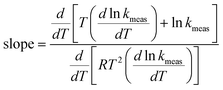 | (12) |
This can easily be simplified to give:Hence it is a general rule that the slope on a Constable plot where the points are obtained at different temperatures will always be 1/RT if all other parameters are kept constant. The gradient of the Constable plot derived in Section 1.1 above, when systematic error was a constant, is merely a special case of this more general rule.
1.3 A systematic error that varies with some other parameter
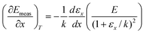
Consider now the case that the Arrhenius parameters ln A and E are constant for a sample, but there is a systematic error in the measurement of rate constant that is a function of some other parameter x (e.g. concentration, pressure, flowrate, or surface coverage).
In this case, the measured rate constant can be written:
where
εx is a systematic error that is a function of parameter
x.
Eqn (3) and (4) still apply, giving:
| |  | (15) |
| |  | (16) |
Hence the values of ln
Ameas and
Emeas now depend on the value of parameter
x (as well as having a weak temperature dependence). Separate points on a Constable plot will therefore be obtained when parameter
x is varied. Note that in this case, unlike the statistical compensation effect due to random errors, there will be a systematic variation in the values of ln
Ameas and
Emeas as the parameter
x is varied.
The gradient on a Constable plot with data measured at different values of x, but the same values of T, will obey:
| |  | (17) |
From
eqn (15) and (16) we have:
| | 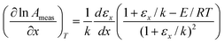 | (18) |
| |  | (19) |
Putting these into
eqn (17) shows that the slope of points on a Constable plot will be:
| | 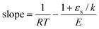 | (20) |
Assuming that the systematic error
εx ≪
k, then:
| | 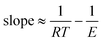 | (21) |
If the temperature range is the same for the kinetic measurements at each value of
x, then this slope will be constant. The effect of the systematic error is thus to induce an apparent compensation effect for a sample with a fixed value of ln
A and
E. It is predicted that the slope of the Constable plot will be somewhat lower than 1/
RTave where
Tave is a weighted average of the temperatures used in the kinetic study. However, it should be noted that in most systems of interest
E is significantly greater than
RTave, and so the slope will be close to 1/
RTave.
The possibility that measured rate constants contain a systematic error that depends on another parameter is quite a common one. For instance, rate constants are sometimes determined by measuring initial rates of reaction when the initial concentration C0 is known. In the particular case of a reaction obeying first-order kinetics:
The measured initial rate of reaction may contain a systematic error εr, either because of the measurement method, or because extrapolation of data is required to determine it. Hence:
Assuming that the concentration C0 is known accurately, then putting eqn (23) into eqn (22) leads to:
Hence the measured rate constant in this example has a systematic error that is a function of initial concentration C0. This corresponds to eqn (14) with the parameter x being initial concentration. The theory above shows that a systematic error in the measurement of initial rate of reaction will therefore cause measured values of activation energy Emeas to vary with C0. A Constable plot constructing from data points measured at different values of C0 will have gradient given by eqn (21).
This result is illustrated in Fig. 2 for a reaction obeying first-order kinetics. Here simulations were performed for a first-order chemical reaction with a fixed value of ln A and a fixed value of E. The rates of reaction were calculated at six temperatures for four different values of initial concentration. A constant error in the rate of reaction was added to the data—this error was taken to be half the magnitude of the rate at the lowest temperature and lowest concentration. The simulated data were then analysed to give measured Arrhenius parameters for each concentration. Even though the true kinetic rate constant does not depend on concentration, the systematic error means that the measured values of Arrhenius parameters do depend on concentration. The results show an apparent compensation effect with the gradient on the Constable plot being that predicted by eqn (21).
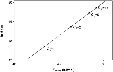 |
| | Fig. 2 The Constable plot resulting from analysis of kinetic data containing a constant systematic error in the measured rate of reaction for a sample with constant Arrhenius parameters. Rates of reaction were simulated for a first-order reaction with a fixed value of ln A (= 20) and E (= 50 kJ/mol) in the temperature range 300–350 K at concentrations C0 = 1, 2, 5 and 10 arbitrary units. A systematic error of 0.5 s−1 was added to the rate of reaction. Calculated rate constants were then analysed to give measured Arrhenius parameters for each concentration. The line shown is a straight line fit through the data points and has a gradient of (1/RT* − 1/E) where T* = 329.0 K which is close to the average temperature used in the study. This is in agreement with the prediction of eqn (21). | |
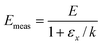
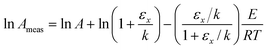
2. The effect of systematic errors in data analysis when the activation energy is a function of another parameter
We now consider what happens if ln A and E for a sample are not constants, but depend on another parameter. For instance, the binding strength of molecules on a surface can be affected by adsorbate-adsorbate interactions and electronic factors, and so the activation energy for desorption can be a function of surface coverage θ. It is also possible that the pre-exponential factor depends on surface coverage. For a first-order process, the rate of desorption from a single type of adsorption site is given by:where the rate constant for desorption obeys:| |  | (26) |
Temperature programmed desorption (TPD) is the most widely used experimental method to determine these Arrhenius parameters.10–12 Analysis of TPD experimental data normally finds that ln Aθ is linearly related to Eθ, i.e. a compensation effect is observed to occur.13 Various physical reasons have been proposed for this compensation effect, none of which are entirely satisfactory.13 In this section, we therefore discuss possible mathematical reasons for the observed compensation effect in this case.
During a single TPD experiment, the rate of desorption is measured while the temperature is increased using a linear heating rate. While there are a variety of methods for analysing TPD data,14,15 the most widely adopted method when the binding strength varies with coverage is to perform a family of TPD experiments at different initial coverages or different heating rates.10,11,16
The actual value of activation energy at coverage θ obeys:
| |  | (27) |
while
eqn (26) can be used to determine ln
Aθ.
In an ideal case, it would be possible from a family of TPD experiments to extract data points that correspond to exactly the same coverage, and then use a plot of ln (rd/θ) against 1/T to get the actual values of Eθ and ln Aθ. However, this is firstly time consuming, and secondly subject to error. In particular, it is very difficult experimentally to ensure that data points are obtained at exactly the same coverage.17,18 This can result in apparent compensation effects, either because the errors are random (as discussed in the accompanying paper),9 or because the errors are systematic (as discussed in Section 1 above). In particular, if the data points analysed are not at exactly the same coverage, then eqn (27) means that:
| |  | (28) |
or equivalently:
| |  | (29) |
Similarly:
| |  | (30) |
The second term on the right-hand side of these equations represents a systematic error in the measured Arrhenius parameters if
dθ/
dT ≠ 0 for the data points analysed.
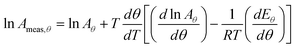
Because of the difficulties in ensuring that the data points on an Arrhenius plot are at exactly the same coverage, an alternative data analysis method is commonly used. This is based on analysing only the early portion of the TPD curve so that the rate of desorption is small.17–19 This experimental method is shown in Fig. 3. The region to be used for the analysis is marked by the solid line, and corresponds to a small change in coverage. Using this method, it is hoped that the activation energy is approximately constant over this region, and that the dθ/dT term is small enough that an Arrhenius plot will give a reasonably reliable value for Eθ for that particular coverage. Repeating the experiment at different initial coverages will measure Eθ and ln Aθ as a function of coverage. However, we show here that this method of analysis creates a systematic error in the value of Arrhenius parameters, even in the limiting case that the change in coverage tends to zero, and that this systematic error causes an apparent compensation effect.
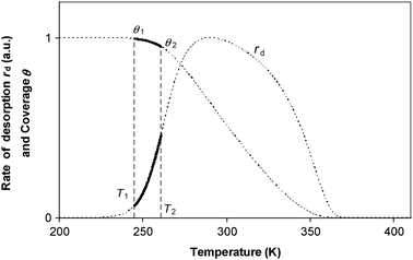 |
| | Fig. 3 The temperature programmed desorption (TPD) experiment measures rate of desorption, rd as a function of temperature as the temperature is increased at a linear rate. The coverage θ drops during the course of the TPD experiment. It has been proposed that analysing the early part of the TPD curve, as shown in the bold solid line, will give an accurate measurement of ln A and E for this coverage. The curves shown in the Figure were obtained by numerical simulation of a system with constant A = 1013 s−1, an activation energy for desorption obeying Eθ = 100–20 θ kJ/mol, with an initial coverage θ0 = 1, and a heating rate of 0.1 K s−1. For this system, the temperature T1 at which θ1 = 0.995 θ0 is found to be 244.9 K, and the temperature T2 at which θ2 = 0.95 θ0 is found to be 261.0 K. | |
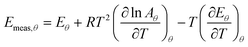
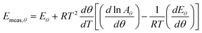
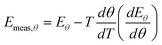
For simplicity, we shall consider a system in which ln A is in fact constant, but Eθ depends on coverage—this is the situation in the numerical simulation results shown in Fig. 3. It is necessary experimentally for there to be a change in coverage for a measurement to be performed. Further, it is impossible to measure very small rates of desorption accurately because they will be subject to random experimental noise and baseline correction errors. For this reason, Fig. 3 shows a region for analysis from 0.995 θ0 down to 0.95 θ0 where θ0 is the coverage at low temperature. For convenience, we shall just consider the two end points to estimate the average gradient of an Arrhenius plot in this region of coverage. The value of Emeas,θ obtained from the two end points of the region will be:
| | 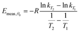 | (31) |
| | 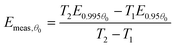 | (32) |
Assuming that
dEθ/
dθ is approximately constant over the range of coverage investigated, then:
| | 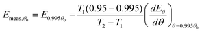 | (33) |
Hence analysis of the early part of a TPD curve, for a system in which ln
A is constant, gives the determined value of
activation energy at
θ0 to be:
| | 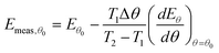 | (34) |
where
T1 is the temperature at which the rate can first be detected accurately, and
T2 is the temperature at which the coverage has changed by Δ
θ. The measured value of pre-exponential factor determined by this method will be:
| |  | (35) |
The second term on the right-hand side of these expressions is the systematic error created by this analysis method. It can be seen that the systematic error in the measured values of Eθ is related to the systematic error in the measured value of ln Aθ. Hence this method of analysis will cause an apparent correlation between ln Aθ and Eθ, and thus a false compensation effect.
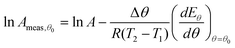
Even in the limit that the change in coverage becomes infinitesimally small, a false compensation effect can still occur. If we consider the case again that ln A is constant, then eqn (29) gives:
| |  | (36) |
However at a particular temperature:
| | 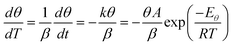 | (37) |
for a system obeying first-order kinetics with a constant heating rate
β. Hence:
| | 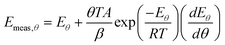 | (38) |
Similarly:
| | 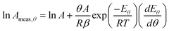 | (39) |
These equations give the values of ln Ameas,θ and Emeas,θ that would be obtained using this analysis method in the limiting case that the change in coverage becomes zero. It can be seen that the systematic error in the value of Emeas,θ depends directly on the systematic error in the value of ln Ameas,θ. Hence, even in this limiting case, the method of analysis can cause a false compensation effect.
We illustrate these predictions by analysing simulated TPD results that are free from experimental errors in order to show the mathematical origin of the compensation effect by this analysis method. The results of the numerical simulations shown in Fig. 3 can be used to construct an Arrhenius plot of ln (rd/θ) against 1/T, for data in the range θ = 0.995 to 0.95, as shown in Fig. 4. The data show a curve, but the analysis method assumes it is a straight line. Analysis of the two end points gives a value for measured activation energy that corresponds to eqn (34). Whilst not practical to do with real experimental data, with the simulations it is possible to analyse the gradient of the tangent when the coverage is exactly 0.995—this corresponds to the “best case” scenario by this analysis method, and it gives a measured activation energy that corresponds to eqn (38). The procedure can then be repeated at different initial coverages. The results of doing so are presented on a Constable plot in Fig. 5.
 |
| | Fig. 4 The bold curve is the result of analysing the TPD data shown in Fig. 3. The change in coverage is from θ1 = 0.995 down to θ2 = 0.95 for a system in which ln A is constant, but Eθ varies according to Eθ = 100–20 θ kJ/mol. Straight line (a) shows the gradient that would be obtained by analysing the two end points, and corresponds to a value for Emeas,θ according to eqn (34). Straight line (b) shows the slope at θ1 = 0.995, the gradient of which corresponds to a value for Emeas,θ according to eqn (38). | |
 |
| | Fig. 5 Results of analysing error-free TPD experimental data for a system in which ln A is constant but Eθ varies with coverage according to Eθ = 100–20 θ kJ/mol, for four different initial coverages. When the region analysed is 0.995 θ0 to 0.95 θ0, the results are shown by squares, with straight line (a) indicating an apparent compensation effect. In the limit that there is no change in coverage for the region investigated, the results are shown by triangles, with straight line (b) indicating an apparent compensation effect. The true values of Arrhenius parameters in this example are shown by crosses and line (c). | |
It can be seen that the analysis method has created an apparent compensation effect, in which ln Ameas,θ has an approximate linear correlation with Emeas,θ even though ln A is in fact constant and the kinetic data is free from error. It is the assumptions behind the analysis method that has created the systematic error. Observed compensation effects when this experimental method is used can thus have a mathematical origin, rather than an underlying physicochemical basis.
3. The effect of analysing overall rates of reaction
In many chemical processes, the overall rate of reaction can be measured but it is not practical to determine an intrinsic rate constant. This may be because the form of the rate law is not known, because the process involves a multi-step mechanism, or because the rate is affected by mass transport limitations. For example, reaction on a heterogeneous catalyst may involve diffusion through pores, adsorption on an active site, surface reaction and desorption steps. It is therefore common practice to fit the overall rate of reaction to the Arrhenius equation to obtain an overall activation energy Eov and an overall pre-exponential factor Aov, defined through the equation:6,20| |  | (40) |
Note that Eov does not necessarily correspond to the activation energy for a single reaction step, because it can contain contributions from all the different steps involved in the overall process.
Values of ln Aov and Eov may be obtained for a family of similar chemical processes in which one reagent is varied, or the catalyst is varied, while keeping other conditions the same. It is also possible to determine values of ln Aov and Eov for the same chemical process, but while varying some other parameter (such as pressure, concentration, flowrate or surface coverage). Experimentally, it is often found that ln Aov is linearly related to Eov.6 One possible reason for this is that the existence of random errors in the measurement of rate of reaction causes the statistical compensation effect as discussed in the accompanying paper.9 This section discusses another reason: that the apparent compensation effect is a result of fitting the overall rate of reaction to the Arrhenius equation, rather than analysing an intrinsic rate constant for an elementary reaction.
The overall activation energy and pre-exponential factor of the process obey:
| |  | (41) |
| |  | (42) |
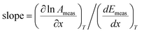
Values of ln Aov and Eov may be determined at different conditions, and the points plotted on a Constable plot to see if the compensation effect occurs or not.
If data points are obtained on the same sample, under the same conditions, with temperature being the only variable, the slope of the Constable plot obeys:
| |  | (43) |
Incorporation of the expressions in
eqn (41) and (42) leads to:
| |  | (44) |
which gives:
This equation has been derived previously for the case that temperature is the only variable.
21
However, if a parameter x other than temperature is varied in order to obtain separate points on the Constable plot, then:
| |  | (46) |
Putting in the expressions of
eqn (41) and (42) leads to:
| | 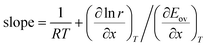 | (47) |
This equation sheds light on when the compensation effect for overall Arrhenius parameters will be observed. For some chemical processes, the second term on the right-hand side is negligible compared to the first term, and so the gradient of the Constable plot is 1/RT. If the temperature range is the same for the kinetic measurements at each value of x, then 1/RT will be constant. This explains why many systems in which the compensation effect is observed have a gradient on the Constable plot of 1/RTave where Tave is the average temperature at which the experiment is performed. In other cases, the second term on the right-hand side of eqn (47) is appreciable—this explains those systems where the gradient on the Constable plot is appreciably different from 1/RTave.
It is instructive to consider a case study to examine further the conditions in which a compensation effect is expected for the overall Arrhenius parameters.
3.1 Case study: unimolecular reaction on a catalyst surface
The compensation effect was first recognised in heterogeneous catalysis2 and continues to be observed experimentally when analysing reaction rates on surfaces.6,22,23 In this case study, we shall consider for simplicity only a simple example—unimolecular reaction on a catalyst surface. Similar conclusions can be derived for more complicated examples, such as a bimolecular reaction by the Langmuir-Hinshelwood mechanism. The reaction mechanism for unimolecular reaction on a surface is:
The rate of reaction will obey:where ks is the surface reaction rate constant, and θA is the surface coverage of species A. Assuming that the Langmuir adsorption isotherm is obeyed then:| |  | (49) |
where KA is the adsorption equilibrium constant for species A, and PA is the partial pressure of A in the gas phase. The constant KA will obey the van't Hoff equation, and so it is straightforward to use eqn (41) to derive the overall activation energy for this mechanism:| | | Eov = Es + ΔHA (1 − θA) | (50) |
where Es is the activation energy of the surface reaction, and ΔHA is the enthalpy of adsorption of species A. We can derive the overall pre-exponential factor using eqn (42), which for this reaction gives:| | 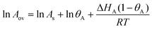 | (51) |
We can now examine different ways in which a unimolecular reaction on a catalyst surface is studied.
3.1.1 Varying P using the same catalyst.
Consider firstly that the overall rate of this reaction is measured on the same sample, over the same temperature range, but at different partial pressures of reactant. Different values of overall Arrhenius parameters will be measured at each partial pressure or, equivalently, each coverage. The slope of the resulting Constable plot can be found using eqn (47) with x taken to be either PA or θA. This gives:| | 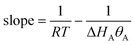 | (52) |
A kinetic compensation effect will be apparent if this slope is roughly constant. This will be the case, with gradient 1/RTave, if RT ≪ |ΔHAθA| for all the conditions used in the study. This situation is frequently the case in practice. On the other hand, if some of the data points in the kinetic study are obtained at very low coverage, then it becomes possible that RT > |ΔHAθA| and the predicted slope become significantly greater than 1/RTave (bearing in mind that the enthalpy of adsorption is negative). This means that the compensation effect is not expected to be observed at very low surface coverages—though the low overall rate of reaction may make this situation difficult to measure in practice.
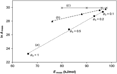
This is illustrated in Fig. 6 which shows the results of a numerical simulation for a unimolecular reaction on a catalyst surface when the experiment is performed at different reactant partial pressures. The results agree with eqn (52). It can be seen that, with the parameters used, the relationship between ln Aov and Eov is approximately linear when the coverage θ > 0.1. Hence a compensation effect will be observed experimentally at these coverages. Deviation from the compensation effect relationship will only occur at low coverages.
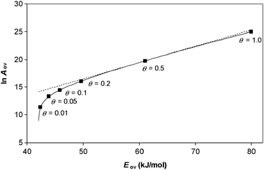 |
| | Fig. 6 Constable plot showing the overall Arrhenius parameters obtained by analysing the temperature dependence of the overall rate of a unimolecular reaction on a catalyst surface. The curve was obtained by simulating the rate of reaction at different reactant partial pressures using parameters |ΔHA| = 38 kJ/mol, ln As = 25, Es = 80 kJ/mol. The analysis was performed at temperature T = 500 K. The straight dashed line is shown to guide the eye—it passes through the point labelled θ = 0.5 and has a gradient predicted by eqn (52) for that coverage. Significant deviation of the curve from the straight line only occurs at low coverage. | |
3.1.2 Effect of varying binding strength to catalyst.
Consider now that the overall rate of the reaction is measured while changing the catalyst (or the reagent), while the same mechanism is still obeyed. The kinetic study is performed at the same partial pressure of reactant and over the same temperature range, and values of ln Aov and Eov are determined for each catalyst.
We shall first consider the case that the binding strength, characterised by the enthalpy of adsorption ΔHA, of the reagent to the catalyst varies from sample to sample, but that the surface reaction rate constant ks is the same for each sample. For simplicity, assume that the adsorption equilibrium constant obeys
| |  | (53) |
with each sample having the same value of
K∞, but a different value of Δ
HA. In this case, the only variable is Δ
HA which then affects equilibrium constant
KA, and thus coverage
θA. We can determine the slope of the Constable plot by using
eqn (50) and (51) with the parameter
x in
eqn (47) chosen to be Δ
HA,
KA or
θA. The result is that the slope of the Constable plot obeys:
| |  | (54) |
If RT ≪ |ΔHAθA| at all the conditions studied, then this equation predicts that the compensation effect will be observed, with a slope of 1/RTave. This explains why the compensation effect can occur for the same reaction but using different catalyst samples, or using the same catalyst but modified reactants. However, if RT ≫ |ΔHAθA| then the slope on the Constable plot will tend to ΔHAθA/R2T2 (which will be a small negative number). This predicts that the compensation effect will not be observed if the catalysts are such that the experiments are performed over a full range of coverages (from low to high). In practice, it may be difficult experimentally to perform the kinetic measurements on samples which have low surface coverages because the overall rate of reaction on them will be small.
The reaction kinetics for a unimolecular reaction on a surface for samples with differing enthalpies of adsorption are illustrated in Fig. 7(a) for a system in which all other parameters are kept constant. The resulting overall Arrhenius parameters are shown in Fig. 7(b). The results agree with eqn (54). The relationship between ln Aov and Eov in this example is approximately linear, and equal to 1/RT, when |ΔHA| > 60 kJ/mol for the example parameters used, corresponding to a coverage θ > 0.15. However, when the binding is weaker the gradient differs significantly from 1/RT. Whether or not a compensation effect is observed experimentally for a family of related catalysts (or related reactants) obeying this mechanism thus depends critically on the range of enthalpies of adsorption that are being investigated.
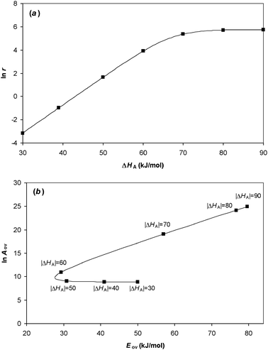 |
| | Fig. 7 (a) The rate of reaction for a unimolecular reaction on a catalyst surface when the enthalpy of adsorption varies. The curve was obtained using parameters ln As = 25, Es = 80 kJ/mol, T = 500 K, PA = 1 bar, K∞ = 10−7bar−1. At high binding strength, the fractional coverage becomes close to unity and so the rate of reaction reaches an asymptote. (b) The Constable plot showing the overall Arrhenius parameters obtained from the temperature dependence of the rate of reaction for samples with differing values of enthalpy of adsorption, with other parameters being constant. The slope in this case is given by eqn (54). | |
3.1.3 Effect of varying rate constant for the surface reaction.
Consider now that the surface reaction Arrhenius parameters ln As and Es vary for a family of catalysts (or reagents), but the enthalpy of adsorption is the same. If the kinetic experiments are conducted at the same pressure and temperature conditions, then the surface coverage will be the same. Inspection of eqn (50) and (51) in this case shows that a compensation effect for the overall Arrhenius parameters will only be observed if there is a genuine compensation effect for the surface reaction Arrhenius parameters. However, it will still need to be checked that any observed compensation effect is not a result of random experimental errors inducing the statistical compensation effect.
3.1.4 Discussion.
There are many examples of the compensation effect being observed when the overall Arrhenius parameters are determined for a catalysed reaction. This case study has identified a possible mathematical reason for this when there are no errors in the kinetic measurements. It can arise because the overall rate of reaction is being analysed, rather than an intrinsic rate constant. If the second term on the right-hand side of eqn (47) is negligible, then the slope of the Constable plot will be 1/RTave. For the catalysis example studied, the second term of eqn (47) is small when the rate of reaction is large—this corresponds to the case that is experimentally easiest to measure. It can be shown using the same method that this is also the case for a bimolecular reaction on a catalyst surface obeying Langmuir-Hinshelwood kinetics. This, together with the statistical compensation effect, explains why families of related catalysts often give data points on a Constable plot that either fall on the same line, or fall on parallel lines.6
The case study has also identified an example physical situation where the observation of a compensation effect for overall Arrhenius parameters, for kinetic data containing no experimental errors, indicates that there is a genuine compensation effect in the underlying true Arrhenius parameters. In such a case, the experimental observation of a compensation effect has physicochemical significance and predictive power.
Conclusions
The accompanying paper demonstrated that random errors in kinetic measurements can cause an apparent compensation effect to occur.9 This paper demonstrates, both theoretically and by numerical simulations, that systematic errors can also cause an apparent compensation effect. Three different possibilities have been discussed in detail.
Firstly, it is shown that systematic errors in kinetic measurements can lead to a variation in the measured value of activation energy, and a correlated variation in the measured value of pre-exponential term. An example case where this occurs is shown in Fig. 2.
Secondly, it is shown that analysis of data in which activation energy is a function of another parameter, such as surface coverage, is not straightforward. In the case of TPD experiments, data can in principle be analysed that correspond to the same surface coverage, but this is difficult to achieve experimentally and any errors in the measured coverage induce an apparent compensation effect. A common analysis method is instead to examine just the early part of the TPD curve, when the coverage has barely changed. However, it is shown here that, even when no experimental errors are present, this method of analysis creates a systematic error which leads to an apparent compensation effect. This occurs even in the limiting case that the coverage does not change over the analysis region. An example where this occurs is shown in Fig. 5.
Thirdly, it is shown that analysis of the temperature dependence of the overall rate of reaction, rather than that of a rate constant, causes a systematic error. Whether a compensation effect will be apparent or not will depend on the magnitude of the two terms of eqn (47). In the case of a unimolecular reaction on a catalyst surface, cases are shown where a compensation effect occurs for mathematical reasons except when the coverage is very low (as shown in Fig. 6 and 7). A case has also been identified where the observation of a compensation effect would imply that there is a genuine compensation effect in the underlying physical parameters.
Overall, this work clarifies many of the misunderstandings in the literature on the kinetic compensation effect. It is now clear that many, but probably not all, of the compensation effects observed in the literature have a mathematical origin—either because of random or systematic errors in the kinetic measurements, or in the assumptions used to obtain the Arrhenius parameters. When the apparent compensation effect has a mathematical origin, there is no need to invoke a physicochemical explanation and the observed effect has little predictive power. Whenever a kinetic compensation effect is observed experimentally, the possibility of it having a mathematical origin should be carefully considered before further conclusions are drawn.
References
- L. Liu and Q.-X. Guo, Chem. Rev., 2001, 101, 673 CrossRef CAS.
- F. H. Constable, Proc. R. Soc. London, 1925, A108, 355 Search PubMed.
- G.-M. Schwab, Adv. Catal., 1950, 2, 251 Search PubMed.
- E. Cremer, Adv. Catal., 1955, 7, 75 Search PubMed.
- A. K. Galwey, Adv. Catal., 1977, 26, 247 CAS.
- G. C. Bond, M. A. Keane, H. Kral and J. A. Lercher, Catal. Rev. Sci. Eng., 2000, 42, 323 CrossRef CAS.
- J. E. Leffler, J. Org. Chem., 1955, 20, 1202 CrossRef CAS.
- K. F. Freed, J. Phys. Chem. B, 2011, 115, 1689 Search PubMed.
- P.J. Barrie, Phys. Chem. Chem. Phys. DOI:10.1069/C1CP22666E , accompanying publication.
- D. A. King, Surf. Sci., 1975, 47, 384 CrossRef CAS.
- J. L. Falconer and J. A. Schwarz, Catal. Rev. Sci. Eng., 1983, 25, 141.
-
J. W. Niemantsverdriet, Spectroscopy in Catalysis: An Introduction, Wiley-VCH, Weinheim, 2000 Search PubMed.
- V. P Zhdanov, Surf. Sci. Rep., 1991, 12, 185 Search PubMed.
- A. M. de Jong and J. W. Niemantsverdriet, Surf. Sci., 1990, 233, 355 CrossRef CAS.
- P. J. Barrie, Phys. Chem. Chem. Phys., 2008, 10, 1688 RSC.
- J. L. Taylor and W. H. Weinberg, Surf. Sci., 1978, 78, 259 Search PubMed.
- J. B. Miller, H. R. Siddiqui, S. M. Gates, J. N. Russell Jr., J. T. Yates Jr., J. C. Trully and M. J. Cardillo, J. Chem. Phys., 1987, 87, 6725 CrossRef CAS.
- D. L. S. Nieskens, A. P. van Bavel and J. W. Niemantsverdriet, Surf. Sci., 2003, 546, 159 CrossRef CAS.
- E. Habenschaden and J. Küppers, Surf. Sci., 1984, 138, L147 CrossRef CAS.
-
I. Chorkendorff and J. W. Niemantsverdriet, Concepts of Modern Catalysis and Kinetics, Wiley-VCH, Weinheim, 2007 Search PubMed.
- H. Lynggaard, A. Andreasen, C. Stegelmann and P. Stoltze, Prog. Surf. Sci., 2004, 77, 71 CrossRef CAS.
- A. Corma, F. Llopis, J. B. Monton and S. Weller, J. Catal., 1993, 142, 97 CrossRef CAS.
- A. K. Galwey, D. G. Bettany and M. Mortimer, Int. J. Chem. Kinet., 2006, 38, 689 Search PubMed.
|
| This journal is © the Owner Societies 2012 |
Click here to see how this site uses Cookies. View our privacy policy here.