The mathematical origins of the kinetic compensation effect: 1. the effect of random experimental errors
Received
19th August 2011
, Accepted 25th October 2011
First published on 14th November 2011
Abstract
The kinetic compensation effect states that there is a linear relationship between Arrhenius parameters ln A and E for a family of related processes. It is a widely observed phenomenon in many areas of science, notably heterogeneous catalysis. This paper explores one of the mathematical, rather than physicochemical, explanations for the compensation effect and for the isokinetic relationship. It is demonstrated, both theoretically and by numerical simulations, that random errors in kinetic data generate an apparent compensation effect (sometimes termed the statistical compensation effect) when the true Arrhenius parameters are constant. Expressions for the gradient of data points on a plot of ln A against E are derived when experimental kinetic data are analysed by linear regression, by non-linear regression and by weighted linear regression. It is shown that the most appropriate analysis technique depends critically on the error structure of the kinetic data. Whenever data points on a plot of ln A against E are in a straight line with a gradient close to 1/RT, then confidence ellipses should be calculated for each data point to investigate whether the apparent compensation effect arises from random errors in the kinetic measurements or has some other origin.
1. Introduction
The temperature dependence of the rates of many chemical processes are normally described well by the Arrhenius equation. This specifies that the rate constant for the process obeys:| | 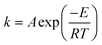 | (1) |
where E is the activation energy, A is the pre-exponential factor, R is the universal gas constant, and T is absolute temperature. The kinetic compensation effect is said to occur when there is a linear relationship between ln A and E for a family of related chemical processes.1
The most common way (but not always the best way, see below) to determine Arrhenius parameters is from a so-called Arrhenius plot of ln ki against 1/Ti where the subscript i indicates each kinetic measurement. A linear fit to the data enables ln A and E to be obtained from the intercept and the gradient. When the experiment is repeated under different conditions, e.g. by varying a reagent, catalyst, or some other parameter, then a different straight line is normally observed. This is illustrated in Fig. 1(a). The different values for the Arrhenius parameters obtained can then be plotted on a graph of ln Aj against Ej, where the subscript j indicates the different conditions employed. This is illustrated in Fig. 1(b). This latter plot is sometimes referred to as a “Constable plot” after its first proponent.2 The kinetic compensation effect occurs when the data points on the Constable plot fall on a straight line.
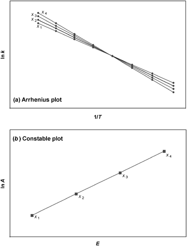 |
| | Fig. 1 (a) An Arrhenius plot is a graph of ln ki against 1/Ti. The gradient enables the overall activation energy E to be obtained, while the intercept on the y-axis gives the value of ln A. Measurements are made on different samples or at different values of some parameter xj. This particular example exhibits the isokinetic relationship. (b) A Constable plot consists of a graph of ln Aj against Ej. The compensation effect occurs if the points obtained at different values of parameter xj fall on a straight line. | |
The kinetic compensation effect is related to, but distinct from, the so-called isokinetic relationship.1,3–7 The isokinetic relationship is obeyed if the rate constants for a family of chemical reactions become identical at a particular temperature (termed the isokinetic temperature, Tiso). This corresponds to separate lines on an Arrhenius plot intersecting at a single point—this is shown in the example data set in Fig. 1(a).
If the kinetic compensation effect is obeyed exactly, then it follows that the isokinetic relationship is obeyed. This is because the kinetic compensation effect implies:
where
α and
β are constants. Combined with the Arrhenius equation, this means:
| | | ln kj = α + βEj − Ej/RT | (3) |
Inspection of this equation shows that separate lines on an Arrhenius plot will intersect at a single point corresponding to ln kiso = α and 1/Tiso = Rβ. Hence strict adherence to the compensation effect predicts the isokinetic relationship. However, in practice, kinetic measurements of many chemical processes show an apparent compensation effect, but no isokinetic relationship.1,4,8 This may be the result of experimental errors in the kinetic measurements as discussed below, or to the sensitivity of the isokinetic relationship to small deviations from exact compensation effect behaviour.7
If the isokinetic relationship is obeyed exactly, then it turns out that the kinetic compensation effect must also be obeyed. This is because a single point of intersection on an Arrhenius plot (at ln kiso and 1/Tiso) implies that each line on the Arrhenius plot obeys:
| | | ln kj = ln kiso + Ej(1/RTiso − 1/RT) | (4) |
This means that the pre-exponential factor for each reaction obeys:
| | | ln Aj = ln kiso + Ej/RTiso | (5) |
Hence it can be seen that the isokinetic relationship implies a linear relationship between ln
Aj and
Ej. Further, the slope of the Constable plot will be 1/
RTiso if the isokinetic relationship is obeyed. However, when random errors are present, it is not always obvious whether separate lines on an Arrhenius plot have a common point of intersection within experimental error. Statistical tests have been proposed to test
experimental data for the existence of the isokinetic relationship in the presence of random errors,
9–12 but many researchers continue to judge the existence of an isokinetic relationship “by eye”. Experimental observation of a statistically significant isokinetic relationship has been claimed to provide good evidence for the existence of a genuine kinetic compensation effect
4,5 though this has been questioned by other workers.
1,13,14
The phenomenon of enthalpy-entropy compensation has also been widely discussed in the literature.1,6,15–17 This is a correlation between the enthalpy change ΔH and entropy change ΔS for a family of chemical reactions. This phenomenon shares many features with the kinetic compensation effect. This is because the method for getting enthalpies and entropies of reaction from thermodynamic equilibrium constants involves plotting a graph of ln K against 1/T. Provided that the enthalpy change ΔH for the reaction does not change greatly with temperature, then the van't Hoff equation predicts that the data points will fall on a straight line, with the gradient giving ΔH, while the intercept gives ΔS for the reaction. This method is thus equivalent to the determination of kinetic parameters by the Arrhenius equation. While this paper concentrates on the kinetic compensation effect, the mathematical analysis is equally appropriate for enthalpy-entropy compensation when the parameters are determined by analysing the temperature dependence of equilibrium constants. However, there is a fundamental difference between the kinetic compensation effect discussed in this paper, and the enthalpy-entropy compensation effect. This is because it is possible in principle to determine ΔH and ΔS values independently of each other. For instance, ΔH can be determined by calorimetric measurements.
2. Aims
The kinetic compensation effect is a widely observed phenomenon in many areas of science, notably heterogeneous catalysis18–21 but also a wide variety of other areas of chemistry.17,22 However, its origins remain the subject of debate in the scientific literature, as discussed in the comprehensive review of Liu and Guo in 2001.1
The main reason for the confusion in the literature is that there are a variety of different manifestations and different reasons for the compensation effect. For some experiments, a kinetic compensation effect can arise for purely mathematical reasons as will be discussed in this work and the accompanying paper. In other experiments, the compensation effect does have an underlying physical significance. For example, one physical explanation for the kinetic compensation effect is that it results from a correlation between the enthalpy change ΔH‡ and the entropy change ΔS‡ on going from the reagents to the transition state of the reaction—it is known from transition state theory that E corresponds to ΔH‡ while ln A is related to ΔS‡. A wide variety of other physical reasons for the kinetic compensation effect have been proposed in the literature for particular situations. However, some of the explanations for observed compensation effects have overlooked the possibility of a purely mathematical origin for that particular case.
The aim of this work and the accompanying paper23 is to explain the possible mathematical origins of the compensation effect. While some of these explanations have been previously described in the literature, research papers continue to be published that do not take them into account. This work extends previous explanations and illustrates them with examples. In this way, it is hoped to dispel the controversy and arguments in the literature on the kinetic compensation effect. Physicochemical explanations for the compensation effect will only need to be sought in those cases when the compensation effect is not arising from a mathematical origin.
This paper is concerned specifically with the effect that random errors in the kinetic measurements have on the determined Arrhenius parameters. It has been shown previously that random errors can generate an apparent compensation effect (referred to as the “statistical compensation effect”) which has no underlying physical significance.24 For this reason, the statistical compensation effect needs to be distinguished carefully from systems that show a compensation effect for other reasons.
This paper first presents the theory behind the statistical compensation effect by considering the correlation between the Arrhenius parameters ln A and E when they are determined by various different regression procedures. The results of some kinetic simulations are then presented to illustrate the mathematical origin of the effect. It will be demonstrated that random errors can indeed induce an apparent compensation effect, and that this possibility needs to be considered before it is concluded that a compensation effect with physicochemical significance is occurring.
3. Theory
It has long been recognised that parameters ln A and E obtained by fitting kinetic data to the Arrhenius equation are not independent of each other.25–31 A rigorous statistical treatment discussing how performing linear fits to data on Arrhenius plots can lead to an apparent compensation effect was described first by Krug and co-workers.24 This paper extends that work to predict and illustrate the effects of random errors on the statistical compensation effect when using both linear and non-linear regression procedures.
Assume that measurements have been made of an intrinsic rate constant ki for a chemical reaction at different temperatures Ti. The Arrhenius equation defines the activation energy E for the reaction, and the pre-exponential factor A through:
| |  | (6) |
Three different regression methods for data analysis are considered here in turn.
3.1 Ordinary linear regression
A plot of ln ki against 1/Ti can be made, as shown in Fig. 1(a), and the data points will fall on a straight line in the absence of experimental noise. With real data, some experimental noise will be present and linear regression is normally performed to obtain the best value of gradient (−E/R) and intercept on the y-axis (ln A).
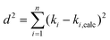
Ordinary least squares linear regression makes a number of assumptions—in particular, the uncertainties in the measured yi values are assumed to obey a Normal distribution with a constant variance, i.e. the errors bars in the ln ki values are taken to have the same magnitude, and there are assumed to be negligible errors in the 1/Ti values. In these circumstances, the objective function is to minimize d2, the sum of the residual squared distances:
| |  | (7) |
Ordinary least squares regression not only provides the “best” values of the fitted parameters, but also enables estimates of the uncertainty in the fitted values to be calculated. For data on a plot of ln
ki against 1/
Ti, the variance in gradient
σ2grad, variance in intercept
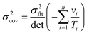
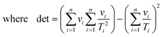
σ2int, and the covariance
σ2cov, obey:
32,33| |  | (8a) |
| | 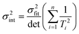 | (8b) |
| | 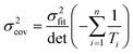 | (8c) |
| |  | (8d) |
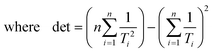
| |  | (8e) |
The values of (−
E/
R) and (ln
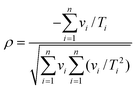
A) determined from regression analysis will be correlated with each other: an increase in the gradient can be compensated to some extent by a reduction in the intercept to give a similar quality fit. The extent of correlation can be quantified by calculating the correlation coefficient between the fitted parameters:
32,33| | 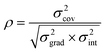 | (9) |
For linear regression of data on a plot of ln
ki against 1/
Ti, the correlation coefficient is:
| | 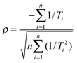 | (10) |
It should be noted that the correlation coefficient depends only on the range of
Ti values used in the experiment. This can be illustrated further using the harmonic mean temperature
Thm defined by:
| |  | (11) |
The squared correlation coefficient can now be written:
| | 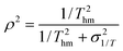 | (12) |
where
σ21/T is the variance in 1/
Ti values. The range of temperatures at which measurements are made is inevitably limited and so, unless ultra-low temperature experiments are being performed,
σ21/T ≪ 1/
T2hm. This means that
ρ2 is close to unity.
For linear regression of kinetic data it can therefore be seen that ρ will be very close to −1 unless the temperature range investigated is impractically large. A correlation coefficient near ±1 means that the uncertainties in the fitted parameters are almost completely dependent on each other, rather than being independent.
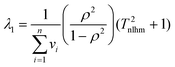
Most computer programs that perform linear regression output standard errors in the fitted parameters; these are calculated from the variances in the gradient and intercept, but ignore the covariance term. However, it is better to calculate a confidence ellipse, which is the region of parameter space within which the fitted parameters are statistically permitted to lie. The lengths of the principal axes of the confidence ellipse depend on the square root of the eigenvalues of the variance-covariance matrix, while the orientation is defined by the eigenvectors.32,33 Expressions for these in the case of linear regression of data on an Arrhenius plot may be found by standard linear algebra. Because all Ti values are much greater than 1 for all practical experiments, terms of order 1/T2hm can be neglected leading to the following expressions for the eigenvalues:
| |  | (13a) |
| |  | (13b) |
Once the eigenvalues are known, the eigenvectors of the variance-covariance matrix can be determined by linear algebra to specify the orientation of the confidence ellipse. These show that, on a graph of (ln
A) against (−
E/
R), the major axis of the confidence ellipse has an orientation defined by tan
θ = 1/
Thm where
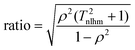
Thm is the harmonic mean of the temperatures at which the kinetic data was obtained. The eigenvalues show that the ratio between the lengths of the principal axes of the confidence ellipse is
| | 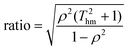 | (14) |
Given that
Thm ≫ 1 and
ρ2 is close to unity, this ratio is very large—it is normally over 1000 for kinetic measurements.
The overall result is that the values of ln A and E determined from the intercept and gradient of the linear regression fit lie within the region of parameter space shown schematically in Fig. 2. The orientation of this confidence ellipse, and its aspect ratio, depend only on the temperatures at which the kinetic experiments were performed. The length of the principal axis of the confidence ellipse depends on how well the experimental data fits the Arrhenius equation and on the number of experimental measurements. The confidence ellipse is very narrow, because eqn (14) implies its aspect ratio is very large, and so the permitted region of ln A and E values approximates a straight line. This means that the uncertainties in the values of ln A and E obtained by ordinary linear regression are directly related by the expression:
| |  | (15) |
where
Thm is the harmonic mean of the temperatures used in the study.
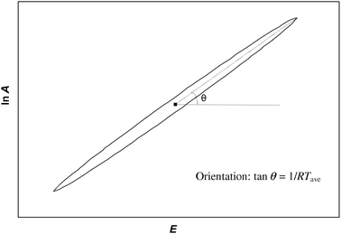 |
| | Fig. 2 Confidence ellipse showing the region of permitted values of ln A and E arising from fitting kinetic data to the Arrhenius equation. Any pair of values lying within the ellipse gives an acceptable fit to the experimental data. The width of the ellipse has been exaggerated for ease of viewing. The ellipse approximates a straight line with orientation defined by tan θ = 1/RTave where Tave is an average of the temperatures values used in the experiment. The average is either the harmonic mean or a weighted harmonic mean depending on the analysis method used. | |
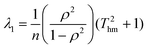
Imagine performing a kinetic study on a family of samples having identical values of ln A and E. Assume that the range of temperatures at which measurements are made is similar for each sample studied. The experimental data contains random errors, which will cause the value of E determined from the linear regression analysis to be for each sample j:
where
E0 is the true value of the activation energy and Δ
Ej arises from random errors in the kinetic measurements on sample
j. However, the effect of
eqn (15) is that the measured value of pre-exponential factor will obey:
| | | ln Aj = ln A0 + ΔEj/RThm | (17) |
where the true values ln
A is denoted by ln
A0. Each sample analysed will have a different random error term Δ
Ej. If a Constable plot of ln
Aj against
Ej is then constructed,
eqn (17) predicts that the points on it will be distributed on a straight line with gradient 1/
RThm. Thus an apparent compensation effect is expected to be observed for a family of samples that have identical values of
E0 and ln
A0.
3.2 Non-linear regression
Before the days of personal computers, doing a straight line fit to obtain intercept and gradient was often the only practical option. A straight line plot also has the advantage of giving an immediate visual impression on whether the model is accurate or not. However, it is recognised that linear regression is not always the best method for analysing data obeying the Arrhenius equation,30,34–37 and that it is often better to perform non-linear regression of data.38
For non-linear regression, the objective function is to minimise d2, the sum of the residual squared distances, on a plot of ki against Ti.
| |  | (18) |
where
ki,calc = exp(ln
A −
E/
RTi). This objective function assumes that the uncertainties in the measured
ki values obey a Normal distribution with a constant variance,
i.e. that the error bars in the
ki values have the same magnitude (in contrast to the assumption for ordinary linear regression of data on an Arrhenius plot). For non-linear regression, the optimum values of the parameters need to be found by iteration. Modern optimisation routines are capable of solving this equation to find the “best” values of ln
A and
E without much difficulty. However, it can be reparameterised if necessary (
e.g. using 1/
Ti as a variable) to give more robust performance in optimisation routines even when the initial guesses are poor.
34,37,39–41
The variance-covariance matrix for the fitted parameters in non-linear regression can be obtained using the local linear approximation.32,38 For non-linear regression to obtain Arrhenius parameters, it is convenient to define the parameter:
| | | νi = k2i,calc = exp[2(ln A − E/RTi)] | (19) |
For non-linear regression, the variance in value of
E/
R, the variance in value of ln
![[thin space (1/6-em)]](https://www.rsc.org/images/entities/char_2009.gif) A
A, and the covariance between these parameters obey:
| | 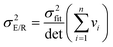 | (20a) |
| | 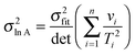 | (20b) |
| |  | (20c) |
| |  | (20d) |
| |  | (20e) |
As before, the extent of the correlation between the parameters obtained by regression can be quantified by calculating the correlation coefficient between the fitted parameters. For non-linear regression of the Arrhenius equation, this is:
| |  | (21) |
As before, unless the temperature range studied is impractically large, this correlation coefficient will be close to −1 indicating the strong correlation between the fitted parameters. It is convenient to define a weighted average harmonic mean temperature
Tnlhm by:
| |  | (22) |
The eigenvalues of the variance-covariance matrix for non-linear regression of data on an Arrhenius plot are (neglecting terms of order 1/
T2nlhm):
| |  | (23a) |
| |  | (23b) |
The aspect ratio of the confidence ellipse on a graph of (ln
A) against (−
E/
R) is:
| |  | (24) |
Because the confidence ellipse approximates a straight line, the overall result for non-linear regression is that the uncertainty in ln
A value is directly related to the uncertainty in
E value through the relationship:
| |  | (25) |
If a kinetic study is performed on samples having identical values of ln
A and
E, and the data analysed by non-linear regression, then the effect of random errors is that the determined Arrhenius parameters obey:
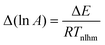
| | | ln Aj = ln A0 + ΔEj/RTnlhm | (26) |
These equations are analogous to the equations derived earlier for ordinary linear regression, but use a weighted harmonic mean as the temperature term. The situation therefore corresponds to that illustrated in
Fig. 2. As before, samples having identical values of ln
A and
E are expected to show an apparent compensation effect because of the existence of random errors, but this time the predicted gradient on the Constable plot will be 1/
RTnlhm.
3.3 Weighted linear regression
When the uncertainties in the yi values obey a Normal distribution but with a different variance for each data point, then it is appropriate to perform weighted regression, rather than ordinary least squares regression.32,33 Weighted regression minimises the objective function:| | 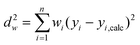 | (27) |
where wi is the weighting of the ith data point. In this case, weighted linear regression is the most convenient method because it has an analytical solution, rather than using an iterative scheme when performing weighted non-linear regression. The appropriate weighting function wi to use for linear regression of data on an Arrhenius plot is the reciprocal of the variance of the uncertainty in ln ki value.
An analogous procedure to that performed in the ordinary linear regression can be performed to get the “best” values of intercept and gradient, the variances and covariance of these parameters, the eigenvalues and eigenvectors of the variance-covariance matrix, and the confidence ellipse. As was the case with the other analysis methods, the result is that the confidence ellipse is very narrow and approximates a straight line. In terms of the Arrhenius parameters, the overall result is that the uncertainty in ln A value is directly related to the uncertainty in E value through the relationship:
| | 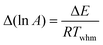 | (28) |
where
Twhm is a weighted harmonic mean temperature given by:
| |  | (29) |
As previously, this predicts that samples having identical values of ln
A and
E will show an apparent compensation effect because of the influence of random errors, because points on the Constable plot will obey
| | | ln Aj = ln A0 + ΔEj/RTwhm | (30) |
The predicted gradient on the Constable plot is 1/
RTwhm as shown in
Fig. 2.
For weighted linear regression of data on an Arrhenius plot, the appropriate weighting function is the reciprocal of the squared standard deviation of the uncertainty in each ln ki value. One particular case is worth considering in more detail. Because d(ln k) = dk/k, for the special case that the variance in ki value is constant, then the standard deviation of the uncertainty ln ki values is proportional to 1/ki, and the appropriate weighting function is wi = k2i. This special case corresponds to the situation in which the assumptions for (unweighted) non-linear regression are valid. For non-linear regression, eqn (26) predicts that the slope on the Constable plot is based on a harmonic mean temperature that has a weighting based on k2i,calc, from eqn (19) and eqn (22), while for weighted linear regression, eqn (30) predicts that the slope of the Constable plot is based on a harmonic mean temperature that has a weighting based on k2i from eqn (29). These two analysis methods are therefore expected to give almost identical results when the variance in ki values is constant.
3.4 Other analysis methods
It is worth commenting that several methods for analysing data using the Arrhenius equation have been proposed that utilise a reference temperature Tref.37,39–42 For instance, one such formulation rewrites the Arrhenius equation in the following form:| | 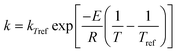 | (31) |
The reference temperature is usually chosen to be the average of the temperatures used in the experimental study. This function has two advantages. Firstly, it is more “well behaved” than original Arrhenius equation. This means that it can be used in least squares fitting routines even when initial guesses of the fitting parameters are poor. Secondly, judicious choice of Tref will minimise the correlation between the fitted parameters kTref and E.37 It is thus sensible to use this formulation if kTref is the parameter of interest. However, in this paper we are concerned with the correlation between Arrhenius parameters ln A and E. When these are derived following fitting of data to eqn (31), it is found that the same correlation between the parameters ln A and E occurs, regardless of the value of Tref chosen, as was the case using the analysis methods discussed earlier.
4. Results
In order to test the theoretical predictions, kinetic data were generated at 11 temperatures in the range 300–400 K for a set of 20 samples that have identical values of ln A0 (taken to be 20) and E0 (taken to be 50 kJ mol−1). A random error was then added to each kinetic data point. This was done in two different ways. In the first data set (data set 1), the random error was assumed to obey a Normal distribution with a variance in the value of ki that was constant (and equal to one half of the value of ki at the lowest temperature). This data set violates one of the assumptions behind linear regression analysis, namely that the errors bars for each ln ki value are not constant, but obeys the assumptions for non-linear regression. In the second data set (data set 2), the random error was assumed to obey a Normal distribution with a variance in the value of ln ki that was constant. This data set obeys the assumptions for ordinary least squares linear regression, but violates the assumption for non-linear regression.
These data sets allow us to explore the sensitivity of the statistical compensation effect to error structure when data analysis is performed by ordinary linear regression, non-linear regression, and weighted linear regression.
4.1 Analysis of data set 1
The most common method of analysing kinetic data is using ordinary linear regression. The results of using this method to analyse data set 1 are shown in Fig. 3(a). Even though the actual values of ln A and E are in fact the same for the 20 samples, an apparent compensation effect in the measured values of ln A and E is evident. This is an example of the statistical compensation effect generated by the presence of random errors in the experimental data. Despite the fact that the kinetic data were analysed at 11 different temperatures (more temperature data points than is normal in experimental studies), the range of E values obtained is appreciable (covering 46–60 kJ mol−1 in this example). If fewer temperatures are used in the kinetic study, then a wider range of E values is obtained.
 |
| | Fig. 3 Analysis of data set 1 by (a) ordinary linear regression; (b) non-linear regression. In both cases, the Constable plot was generated from 20 samples of data having identical values of ln A0 (= 20) and E0 (= 50 kJ/mol). Kinetic data was generated at 11 temperatures, and random experimental noise added to it. For this data set, the standard deviation of the Normal distribution for the uncertainty in ki value was constant. The straight lines demonstrate that the effect of random experimental noise is to cause an apparent compensation effect. | |
The assumption for ordinary linear regression that the error bar in ln ki value is constant is violated for this data set. This has two effects. Firstly, it causes the average value of ln A and E on the Constable plot in Fig. 3(a) to have a systematic error: the average values are Eave = 51.1 kJ mol−1 and ln Aave = 20.3, rather than the true values of 50 kJ mol−1 and 20 respectively. The reason for this is that the true error bar of ln ki is not really symmetrical: at low values of ki, the error bar of ln ki should be greater in the negative direction than the positive direction. This makes it more likely that the gradient of the Arrhenius plot (and thus the value of E determined) is slightly greater than the actual value. Secondly, the violation of the assumptions for ordinary linear regression means that the prediction of the gradient of the Constable plot by eqn (17) is not exact. In this case, the gradient 1/RT* of the Constable plot corresponds to a value of T* = 366.9 K, while the harmonic mean temperature is Thm = 347.1 K for this data set. Similar analysis results were obtained on a second independent data set containing random errors generated under identical conditions.
It is worth commenting that Krug and co-workers24 proposed that the statistical compensation effect could be inferred by performing a statistical test to see whether the slope of the Constable plot was 1/RThm using an appropriate confidence interval. However, the results presented here show that significant deviations from this predicted gradient will occur if the assumptions behind ordinary linear regression are violated. The proposed test is therefore not a rigorous one for establishing whether the statistical compensation effect is occurring or not.
The results of analysing data set 1 using non-linear regression are shown in Fig. 3(b). The same data set was also analysed using weighted linear regression with weighting function wi = k2i as discussed in the theory section. The results obtained by weighted linear regression analysis correspond almost exactly with those obtained by non-linear regression. The main conclusion is that the scatter of the points for this data set is far smaller using non-linear regression, or weighted linear regression, than when using ordinary linear regression. The points are all within 0.6 kJ mol−1 of the actual E0 value. The gradient of the Constable plot agrees with the prediction of eqn (26), specifically the gradient is 1/RT* where T* = 392.8 K, while the weighted harmonic mean temperature Twhm = 391.9 K.
This work thus confirms previous observations that the values of ln A and E, and their uncertainties, obtained by fitting data to the Arrhenius equation depend on the method of analysis.30,43 It is clear that superior results are obtained for data set 1 using non-linear regression or weighted linear regression. This is not surprising because the error structure used to generate this data set violates the assumptions for ordinary linear regression analysis, and obeys the assumptions for non-linear regression.
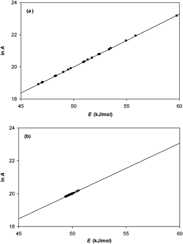
4.2 Analysis of data set 2
The same regression techniques were used to analyse data set 2. These data were generated so that the assumptions for ordinary linear regression were obeyed, while those for non-linear regression were violated. The results are shown in Fig. 4.
 |
| | Fig. 4 Analysis of data set 2 by (a) ordinary linear regression; (b) non-linear regression. In both cases, the Constable plot was generated from 20 samples of data having identical values of ln A0 (= 20) and E0 (= 50 kJ/mol). Kinetic data was generated at 11 temperatures, and random experimental noise added to it. For this data set, the standard deviation of the Normal distribution for the uncertainty in ln ki value was constant. The straight lines demonstrate that the effect of random experimental noise is to cause an apparent compensation effect. | |
For ordinary linear regression, the range of calculated E values ranges from 48.2 to 52.5 kJ mol−1, and the observed gradient 1/RT* on the Constable plot corresponds to a value of T* = 347.0 K. This agrees well with the actual activation energy and the harmonic mean temperature for this data set (E = 50 kJ mol−1; Thm = 347.1 K), and demonstrates that eqn (17) is accurate when the assumptions for ordinary linear regression are valid.
For data set 2, non-linear regression analysis gives a wide range of calculated E values (42.7 to 69.1 kJ mol−1 in this case). The observed gradient 1/RT* of the Constable plot corresponds to a value of T* = 379.8 K. This is close, but not identical, to that predicted by eqn (26): some deviation is expected because eqn (26) was derived assuming the assumptions for non-linear regression were valid.
For data set 2, it is clear that superior results are obtained using ordinary linear regression. This is not surprising because the error structure used to generate the data set obeys the assumptions for ordinary linear regression analysis, and violates the assumptions for non-linear regression.
5. Discussion
This paper demonstrates, both theoretically and by simulations, that random errors in kinetic measurements can cause an apparent compensation effect (the “statistical compensation effect”). The straight line fit between ln A and E values on a Constable plot is excellent—indeed, the correlation coefficient R2 for the data reported in Fig. 3 and 4 is greater than 0.9995 in each case. The best method of data analysis to reduce the statistical compensation effect depends critically on the error structure of the kinetic measurements. In some cases, it is clear that non-linear regression, or weighted linear regression, is superior to ordinary linear regression, while the converse can also be true. If the error structure is known, and the errors bars have different magnitude for each data point, then weighted linear regression is the most appropriate analysis technique. In the general case, if reliable error bars for each data point are not known, then the effect of applying a regression procedure when the assumptions are not valid is complex.30,37,44–46 If reliable errors bars are not known for each data point, we recommend that the data are analysed by both ordinary linear regression and non-linear regression to see whether there are significant differences between the results.
The statistical compensation effect means that kinetic data on identical samples will produce a straight line on a Constable plot with gradient 1/RTwhm, where Twhm is a weighted harmonic mean of the temperatures used in the study. If analysis is performed by ordinary linear regression the gradient will only be 1/RThm if the assumptions for ordinary linear regression are valid.
It should be noted that an apparent compensation effect with gradient 1/RTwhm implies that the isokinetic relationship is approximately obeyed, with an apparent isokinetic temperature of Twhm. Hence random errors in kinetic measurements can cause an apparent isokinetic relationship. The effect of random errors, when analysing kinetic data on identical samples, is that the straight lines of best fit on an Arrhenius plot come close to intersecting at the same temperature. However, in this case it is just as likely statistically that the lines on an Arrhenius plot lie exactly on top of each other, as that they intersect at a single temperature.
The statistical compensation effect can also arise when kinetic data on a single sample are obtained while varying another parameter x (such as pressure, concentration, or coverage). If the compensation effect arises from random errors in the kinetic data alone, then no systematic variation in the measured value of E with parameter x is expected to occur. Observation of a systematic variation of E with x is indicative of another form of compensation effect; for instance, it might result from systematic errors as discussed in the accompanying paper.23
Whenever a compensation effect is observed with a gradient on the Constable plot close to 1/RTwhm, error analysis should be performed to investigate whether it arises from random errors in the kinetic measurements. This involves calculation of confidence ellipses for each data point on the Constable plot. In some cases in the literature, a compensation effect has been reported, but calculated confidence ellipses overlap with each other. In these cases, it is likely that the apparent compensation effect has a mathematical origin, arising purely from the experimental errors in the kinetic measurements. Attempts to ascribe a physicochemical reason for the compensation effect in such cases are flawed.
References
- L. Liu and Q.-X. Guo, Chem. Rev., 2001, 101, 673 CrossRef CAS.
- F. H. Constable, Proc. R. Soc. London, 1925, A108, 355 Search PubMed.
- R. C. Petersen, J. Org. Chem., 1964, 29, 3133 CrossRef CAS.
- R. K. Agrawal, J. Therm. Anal., 1986, 31, 73 Search PubMed.
- W. Linert and R. F. Jameson, Chem. Soc. Rev., 1989, 18, 477 RSC.
- W. Linert, Chem. Soc. Rev., 1994, 23, 429 RSC.
- M. P. Suárez, A. Palermo and C. M. Aldao, J. Therm. Anal., 1994, 41, 807 Search PubMed.
- Z. Karpinski and R. Larsson, J. Catal., 1997, 168, 532 Search PubMed.
- O. Exner, Collect. Czech. Chem. Commun., 1972, 37, 1425 CAS.
- O. Exner and V. Beranek, Collect. Czech. Chem. Commun., 1973, 38, 781 CAS.
- R. R. Krug, Ind. Eng. Chem. Fundam., 1980, 19, 50 Search PubMed.
- W. Linert, R. W. Soukup and R. Schmid, Comput. Chem., 1982, 6, 47 CrossRef CAS.
- J. Zsakó and K. N. Somasekharan, J. Therm. Anal., 1987, 32, 1277 Search PubMed.
- N. Koga and J. Šesták, Thermochim. Acta, 1991, 182, 201 CrossRef CAS.
- R. Lumry and S. Rajender, Biopolymers, 1970, 9, 1125 CrossRef CAS.
- K. Sharp, Protein Sci., 2001, 10, 661 CrossRef CAS.
- K. F. Freed, J. Phys. Chem. B, 2011, 115, 1689 Search PubMed.
- G.-M. Schwab, Adv. Catal., 1950, 2, 251 Search PubMed.
- E. Cremer, Adv. Catal., 1955, 7, 75 Search PubMed.
- A. K. Galwey, Adv. Catal., 1977, 26, 247 CAS.
- G. C. Bond, M. A. Keane, H. Kral and J. A. Lercher, Catal. Rev. Sci. Eng., 2000, 42, 323 CrossRef CAS.
- J. E. Leffler, J. Org. Chem., 1955, 20, 1202 CrossRef CAS.
- P.J. Barrie, Phys. Chem. Chem. Phys. 10.1039/C1CP22667C , accompanying publication.
- R. R. Krug, W. G. Hunter and R. A. Grieger, J. Phys. Chem., 1976, 80, 2341 CrossRef CAS.
- R. C. Petersen, J. H. Markgraf and S. D. Ross, J. Am. Chem. Soc., 1961, 83, 3819 CrossRef CAS.
- R. F. Brown, J. Org. Chem., 1962, 27, 3015 CAS.
- O. Exner, Collect. Czech. Chem. Commun., 1964, 29, 1094 CAS.
- J. E. Leffler, J. Org. Chem., 1966, 31, 533 CAS.
- G.-M. Schwab, J. Catal., 1983, 84, 1 Search PubMed.
- K. Héberger, S. Kemény and T. Vidóczy, Int. J. Chem. Kinet., 1987, 19, 171 CAS.
- A. Cornish-Bowden, J. Biosci., 2002, 27, 121 Search PubMed.
-
N. R. Draper and H. Smith, Applied Regression Analysis, Wiley, New York, 1998 Search PubMed.
-
S. A. Glantz and B. K. Slinker, Primer of Applied Regression and Analysis of Variance, McGraw-Hill, New York, 2001 Search PubMed.
- N. H. Chen and R. Aris, AIChE J., 1992, 38, 626 Search PubMed.
- R. L. Curl, AIChE J., 1993, 39, 1420 Search PubMed.
- O. E. Rodionova and A. L. Pomerantsev, Kinet. Catal., 2005, 46, 305 Search PubMed.
- M. Schwaab and J. C. Pinto, Chem. Eng. Sci., 2007, 62, 2750 Search PubMed.
-
Y. Bard, Nonlinear Parameter Estimation, Academic, New York, 1974 Search PubMed.
- G. E. P. Box, Ann. N. Y. Acad. Sci., 1960, 86, 792 Search PubMed.
- D. J. Pritchard and D. W. Bacon, Chem. Eng. Sci., 1975, 30, 567 Search PubMed.
- A. K. Agarwal and M. L. Brisk, Ind. Eng. Chem. Process Des. Dev., 1985, 24, 203 Search PubMed.
- E. C. W. Clarke and D. N. Glew, Trans. Faraday Soc., 1966, 62, 539 RSC.
- M. E. Brown and A. K. Galwey, Thermochim. Acta, 2002, 387, 173 Search PubMed.
- N. Brauner and M. Shacham, Chem. Eng. Process., 1997, 36, 243 Search PubMed.
- R. Klička and L. Kubáček, Chemom. Intell. Lab. Syst., 1997, 39, 69 CrossRef CAS.
- R. Sundberg, Chemom. Intell. Lab. Syst., 1998, 41, 249 CrossRef CAS.
|
| This journal is © the Owner Societies 2012 |
Click here to see how this site uses Cookies. View our privacy policy here.