Multilayer perceptron neural network for flow prediction

Abstract

Artificial neural networks (ANNs) have proven to be a tool for characterizing, modeling and predicting many of the non-linear hydrological processes such as rainfall-runoff, groundwater evaluation or simulation of water quality. After proper training they are able to generate satisfactory predictive results for many of these processes. In this paper they have been used to predict 1 or 2 days ahead the average and maximum daily flow of a river in a small forest headwaters in northwestern Spain. The inputs used were the flow and climate data (precipitation, temperature, relative humidity, solar radiation and wind speed) as recorded in the basin between 2003 and 2008. Climatic data have been utilized in a disaggregated form by considering each one as an input variable in ANN₁, or in an aggregated form by its use in the calculation of evapotranspiration and using this as input variable in ANN₂. Both ANN₁ and ANN₂, after being trained with the data for the period 2003–2007, have provided a good fit between estimated and observed data, with R² values exceeding 0.95. Subsequently, its operation has been verified making use of the data for the year 2008. The correlation coefficients obtained between the data estimated by ANNs and those observed were in all cases superior to 0.85, confirming the capacity of ANNs as a model for predicting average and maximum daily flow 1 or 2 days in advance.

---

Environmental impact

This manuscript predicts 1 or 2 days ahead the average and maximum daily flow of a river in northwestern Spain. The flow and climate data recorded in the basin between 2003 and 2008 have been used as data inputs. Climatic data have been utilized in a disaggregated form considering each one as an input variable (ANN₁) or in an aggregated form by its use in the calculation of evapotranspiration and using this as input variable (ANN₂). These results are valuable for the proper management of water resources; tools are needed to evaluate in advance the dynamics of river systems for mitigating the potential impacts of drought on water supply and damage caused by flooding.

Introduction

The impact of climate change on water resources depends largely on the changes that occur in rainfall and on the climatic variables that govern evapotranspiration.

Current predictions suggest that rainfall in Galicia tends to manifest springs and summers with less precipitation and increased rainfall during autumn and winter. For the A₁B emissions scenario predicted by the HadCM3 model, precipitation increases will average above 25%.¹ Moreover, under the same scenario, the HadCM3 model shows mid 21st century temperature predictions with increases exceeding 2.5 °C during summer.¹ These variations in weather conditions involve on the one hand, an increase in summer drought (lower rainfall and higher evapotranspiration) and on the other hand an increased frequency of flooding events during winter months.

Given these perspectives, for proper management of water resources, tools are needed to evaluate in advance the dynamics of river systems to mitigate the potential impacts of drought on water supply and damage caused by flooding.

The complex correlations and non-linearity between climatic, edaphic and geomorphologic variables and hydrologic response of watersheds, results in the use of physical-based models that require a high level of information about the spatial distribution of the basin's physical characteristics and, in most cases, have historical data for model calibration.² These facts, together with the uncertainty of the estimates, have meant that empirical models have been employed as alternative and widely accepted practical methods for hydrological analysis. Empirical models are black-box models with an ability to accurately simulate non-linear dynamic systems.³

Artificial neural networks (ANNs) have proven to be a suitable empirical tool for characterizing, modeling and predicting many non-linear hydrological processes such as rainfall-runoff, groundwater evaluation, severity of droughts or simulation of water quality.^4,5 Neural networks have also been used in aerobiological studies in order to achieve predictive models to improve daily pollen concentration forecast.^6,7

ANNs can be applied to simulate different processes. Recently, some ANNs have been implemented in engineering processes related to wine and vinegar fabrication.⁸ ANNs can also be applied to simulate different processes in chemical engineering.^9–11

ANNs are merely an artificial and simplified model of the human brain. One could define an ANN as a system for information processing whose basic unit is inspired by the fundamental cell of the human nervous system.^12,13 ANNs were originally an abstract simulation of the biological nervous systems, consisting of a set of units called ‘neurons’ or ‘nodes’ connected to each other.¹⁴ The implemented model is based on a perceptron network. The operation of such networks is carried out in two phases: a first phase, presenting the inputs and outputs, and a second one in which the algorithm compares the actual output with the desired output. The difference between them is an error that is propagated backward from the output neuron to the input neurons allowing the adaptation of the network, facilitating in this way the learning process.¹⁵

This paper has analyzed the efficiency of an ANN to forecast 1 or 2 days ahead the average daily (Q_mean+1 and Q_mean+2) and maximum daily (Q_max+1 and Q_max+2) flow in a forest basin from hydrological (maximum and average flow) and meteorological data (solar radiation, air temperature, wind and relative humidity) at t = 0.

Materials and methods

Description of the study basin

The study basin is located in Toén (Galicia, NW Spain). The area average temperature is 14.5 °C and normal annual rainfall is 817 mm. The exit of the basin is located at coordinates 42° 16′ 35′′ N, 7° 59′ 4′′ W where it is drained by the stream of Fragoso, a tributary of the Minho river on its southern slope. The geological material is shale, developing from which is a shallow soil of loamy texture: sand 47%, silt 33%, clay 20%.

The basin has an area of 42.9 hectares, an average height of 510 m and an average gradient of 25.1%. It is a forest basin 65.7% of it being occupied by a plantation of Pinus pinaster, 13.3% by ripisilva forest, and 13.0% by scrubland.

In February 2003 an automatic gauging station was installed at the point of closure of the basin, consisting of a landfill in V of 60 degrees and a capacitive probe connected to a datalogger Starlog (Unidata Australia®) that records the average level of the river at five minutes intervals. A complete automatic weather station has also been installed equipped with a temperature and humidity sensor HMP45A (Vaisala®), a CMP-11 pyranometer (Kipp Zonen®), a 107H anemometer (Ornytion®), and a ARG100 rain gauge (Campbell Sci®), all connected to a Starlog datalogger (Unidata Australia®) that stores recorded data every five minutes.

Fig. 1 shows the location of the basin, indicating both the position of the weather station and the gauging station.

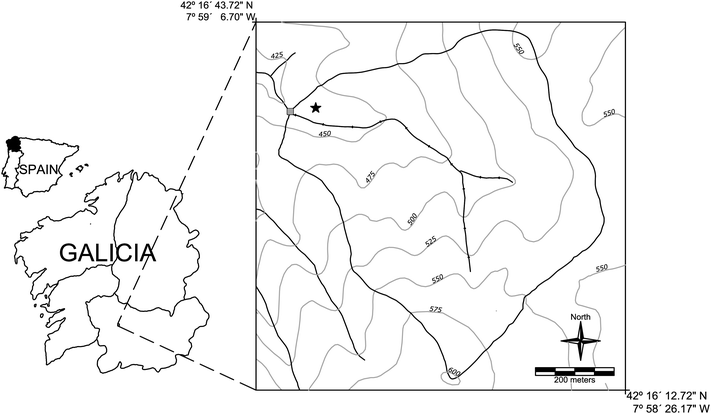Fig. 1 Location map of the basin. The star marks the position of the meteorological station and the square the position of the gauging point.

Methods

To estimate the average flow (Q_mean) and the maximum flow rate (Q_max) from the stream of Fragoso, a model based on ANNs technology was chosen. The equipment used was an Intel Core 2 Quad processor with 4 GB of memory RAM computer using multiple virtual machines in parallel with Xen in order to achieve higher computing performance.

The model consists of the implementation of an ANN formed by various layers of neurons (Fig. 2). An initial layer of neurons which collect data in the input variables, a layer, or more, of intermediate neurons where ‘learning’ operations would be conducted, and a layer of output neurons, where the desired value is obtained. During the training phase the ANN ‘studies’ the relationships between inputs and outputs through an algorithm that compares the results of the training data with the experimental values. If the error is within the training set, it is finalized, otherwise the training continues until reaching the set error.

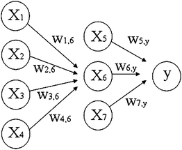Fig. 2 Diagram of a perceptron network consisting of an input layer with four neurons, a hidden or middle layer of three neurons and an output layer consisting of a neuron. W represents the weights between different neurons in each layer.

To estimate the average and maximum daily flow through ANN, a model of the multilayer perceptron type was opted for with supervised training in which ANN training data consist of input and output variables. In the training phase of each of the ANNs, records of the period 2003 to 2007 have been used, these data are formed composed of 8 input variables: precipitation daily data (P, mm), incident solar radiation (R_i, W m⁻²), maximum temperature (T_max, °C), average temperature (T_mean, °C), minimum temperature (T_min, °C), relative humidity (RH, %), wind speed (U, m s⁻¹) and flow at time zero (Q₀, L s⁻¹). The ANNs are designed with an intermediate layer of 3 neurons and one output neuron, average flow expected 2 or 1 days ahead (Q_mean+2, Q_mean+1) or maximum flow expected 2 or 1 days ahead (Q_max+2, Q_max+1). This ANN group has been called ANN₁.

A second group of ANN (ANN₂) has also been tested, which instead uses the input climatic variables (P, R_i, T_max, T_mean, T_min, RH and U) and the potential evapotranspiration (ET₀) obtained by the Penman–Monteith equation.^16–19

where Rn is the net radiation, T is temperature, G is heat flow, U is wind speed, e is the vapor pressure (the subindex a corresponds with the actual value and s is the value in saturation and their difference represents the vapour pressure deficit of the air), Δ represents the slope of the saturation vapor pressure temperature relationship and γ is the psychrometric constant. The learning process of the developed ANNs might be described as follows:

Each of the neurons in the input layer contains the data for each variable and presents them as an input vector

x^p = (x^p₁,x^p₂,…,x^p_N)^T. (2)

This input vector is propagated to the intermediate layer using the following propagation rule:

where N is the number of input neurons of the network, w_ji is the value of the weight of the connection between neuronj of the input layer and neuroni of the middle layer, and b_i is the value of bias associated with neuroni.

Considering that the activation value of neuroni is a function of the input vector, we can say that the output of it is given by:

y^p_i = F_i(s^p_i) (4)

Similarly, for a neuronk of the output layer, the equations that determines its activation state are:

y^p_k = F_k(s^p_k) (6)

where L is the number of neurons in the intermediate layer, w_ik is the weight value of the connection between neuroni of the intermediate layer and neuronk of the output layer, and b_k is the value of the bias associated to the neuronk.

We calculate the error term for the output neuron by eqn (7)

If the error is close to the established value, the ANN training ends here. For non-compliance with established margins the process would be repeated until the desired error is reached.

The activation equation used in this ANN is the sigmoidal or logistic function.

After training the ANN and subsequent verification of the training data correlation its operation was proven with validation data for the year 2008.

The goodness of fit between the flow rate predicted by the ANNs and the flow recorded was evaluated by the root mean squared error (RMSE):

where N is the data number, Y represents the estimated values and X represents the observed values.

Results and discussion

Precipitation and average and maximum daily flow values recorded from March 2003 to September 2008 are shown in Fig. 3. The average annual flow during the years of study showed high variability. In the year 2004/05 the average annual flow reached only 1.2 L s⁻¹ and the maximum daily flow was 3 L s⁻¹. By contrast, the year 2006/07 average annual flow was 7.2 L s⁻¹ and the maximum daily flow was 64 L s⁻¹ (Table 1). This high variability of annual flow is related to precipitation, this way, the linear correlation coefficient between annual precipitation and average annual flow has a value of 0.94 for the period 2003/04 to 2007/08.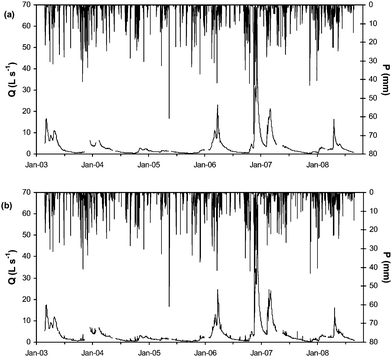

Fig. 3 Daily average flow (a), daily maximum flow (b) and daily precipitation recorded in the basin during the study period.

Table 1 Average annual flow (L s⁻¹), maximum daily flow (L s⁻¹) and annual precipitation (mm) recorded in the basin during the study period. (*) Data for the year 2002/03 extending from March 2003 to September 2003.

Year	Q mean	Q max	P/mm
2002/03^*	4.51	17.5	476.9
2003/04	2.01	6.8	818.7
2004/05	1.19	3.0	633.0
2005/06	2.92	24.6	930.7
2006/07	7.20	64.3	1233.8
2007/08	2.28	15.9	789.6

---

The average and maximum daily flow and weather data recorded between February 2003 and December 2007 have been used to train the ANN₁ in predicting the average and maximum daily flow 1 and 2 days ahead. Fig. 4 and 5 show the average flow and daily maximum flow recorded during the training period and the values obtained by the ANN₁ for that period 2 days ahead (Q_mean+2 and Q_max+2).

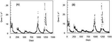Fig. 4 Average daily flow (Q_mean) for the training period of the ANN₁ (A) and average daily flow calculated by the ANN₁ two days ahead (Q_mean+2) after training (B).

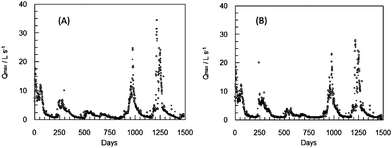Fig. 5 Maximum daily flow rate (Q_max) for the training period of the ANN₁ (A) and maximum daily flow rate calculated by the ANN₁ two days ahead (Q_max+2) after training (B).

Table 2 contains the estimates of the goodness of fit between the observed values and the predicted by ANN₁ for the average and maximum daily flow 1 and 2 days. R² values of the ANN₁ of Q_mean+2 and Q_max+2 was 0.977 and 0.955 respectively, and the RMSE of 1.016 and 1.285 L s⁻¹ respectively.

Table 2 Parameters of fit between the predicted flow after ANN₁ training for one or two days ahead and the recorded flow. n is the number of used values, b and a the slope and the origin of the regression line, R² the determination coefficient and RMSE the root mean squared error

	n	a	b	R ^2	RMSE
Q mean+1	1504	0.191	0.965	0.988	0.596
Q max+1	1504	0.185	0.906	0.971	1.025
Q mean+2	1489	0.652	0.972	0.977	1.016
Q max+2	1489	0.503	0.898	0.955	1.285

---

For estimating the values of average and maximum daily flow rate at 1 day (Q_mean+1 and Q_max+1), the R² value was higher than in the case of the estimate to two days. The same applies to the RMSE, in this case, the value for the average flow is only 0.596 L s⁻¹ (Table 2).

Therefore, the values obtained from the efficiency estimates for the average and maximum flow prediction by ANN₁ have been satisfactory for both 1 and 2 days ahead. The R² value obtained was in all cases superior to 0.95 and the RMSE less than 1.5 L s⁻¹.

Having established the proper functioning of ANN₁, its validity was then checked through the prediction of average and maximum flow rates at 1 and 2 days, making use of the validation period for the year 2008.

The results obtained are shown in Fig. 6 and 7. In general, there is a good fit between values observed and predicted by ANN₁, both for low flows and level rise periods. Similarly forecasts at 1 and 2 days ahead are satisfactory in both cases, although the estimates of the goodness of fit are slightly better in the case of one day ahead (Table 3).

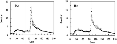Fig. 6 Average (A) and maximum (B) daily observed (●) and estimated by the ANN₁ (dotted line) flow two days ahead during the validation period.

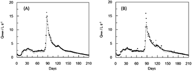Fig. 7 Average (A) and maximum (B) daily observed (●) and estimated by the ANN₁ (dotted line) flow one day ahead during the validation period.

Table 3 Parameters of fit between the predicted flow for the ANN₁ validation period for one or two days ahead and the recorded flow. n is the number of values, b and a the slope and the origin of the regression line, R² the determination coefficient and RMSE the root mean squared error

	n	a	b	R ^2	RMSE
Q mean+1	210	−0.0915	0.9771	0.963	0.604
Q max+1	210	0.1040	0.880	0.971	0.668
Q mean+2	210	0.2952	0.9386	0.885	1.016
Q max+2	210	0.5347	0.8458	0.896	1.285

---

The values of the statistical criteria used for analyzing the quality of flow estimation by ANN₁ at 1 and 2 days are displayed in Table 3.

Analysis of the weight of system variables shows that the dominant variable is the solar radiation, R_i (Table 4), with an excessive weight if we try to relate the weights of the variables in terms of their physical meaning and the importance presented in theoretical predictive models. This high importance of R_i is related to the statistical weight of the above-mentioned variable, and along the time series there is a wide range in its variability (26.5–253.1 W m⁻²) compared with other variables, which a priori should have a greater weight in decision making. Variables with a low range of variability (e.g.precipitation, ranging from 0–69.2 mm) show a smaller statistical weight in the ANN₁ decision making process.

Table 4 Importance of variables for each of the developed ANN₁

ANN for Qmean+2		ANN for Qmax+2
Solar radiation (Ri)	56.37	Solar radiation (Ri)	53.03
Average Temperature (Tmean)	50.73	Flow at time zero (Q0)	40.73
Relative Humidity (RH)	32.04	Minimum temperature (Tmin)	20.91
Maximum temperature (Tmax)	17.69	Average Temperature (Tmean)	14.21
Flow at time zero (Q0)	16.57	Maximum temperature (Tmax)	13.75
Minimum temperature (Tmin)	15.90	Relative Humidity (RH)	8.41
Precipitation (P)	8.80	Precipitation (P)	5.15
Wind speed (U)	7.75	Wind speed (U)	2.65

---

ANN for Qmean+1		ANN for Qmax+1
Flow at time zero (Q0)	20.89	Solar radiation (Ri)	21.45
Solar radiation (Ri)	17.28	Wind speed (U)	18.19
Relative Humidity (RH)	13.60	Maximum temperature (Tmax)	15.07
Maximum temperature (Tmax)	9.04	Flow at time zero (Q0)	14.91
Average Temperature (Tmean)	8.68	Relative Humidity (RH)	13.41
Wind speed (U)	6.73	Precipitation (P)	12.12
Precipitation (P)	6.72	Average Temperature (Tmean)	7.94
Minimum temperature (Tmin)	0.94	Minimum temperature (Tmin)	4.45

---

In order to reduce the number of input variables, potential evapotranspiration (ET₀) was chosen to be included as the only climate variable, in addition to precipitation. This variable can be calculated from the previously used variables (R_i, U, RH, T_meanT_max and T_min) by eqn (1). Besides this method of ET₀ calculation, which involves using a large number of weather parameters not available in many weather stations, it is also possible to determine it by simpler expressions with fewer parameters, which have been used successfully in many regions.

Therefore, in this case we have evaluated the efficacy of ANNs in predicting the flow of a basin using as input variables P, Q and ET₀. This involves reducing the number of input neurons from 8 (if ANN₁) to 3 (to these networks, which we will call ANN₂).

Fig. 8 and 9 show the estimates obtained by ANN₂ for the average and maximum flow one day ahead for the training period. In both cases results were satisfactory, and the proper adjustment for the high flows period is particularly interesting .

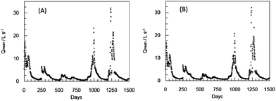Fig. 8 Average daily flow rate (Q_mean) recorded during the ANN₂ training period (A) and average daily flow rate calculated by the ANN₂ one day ahead (Q_mean+1) after training (B).

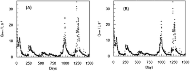Fig. 9 Maximum daily flow rate (Q_max) recorded during the ANN₂ training period (A) and maximum daily flow rate calculated by the ANN₂ one day ahead (Q_max+1) after training (B).

Later, after training, the effectiveness of ANN₂ for forecasting the flow rate was evaluated during the validation period for the year 2007.

The results were equally satisfactory as for the validation period as shown in Fig. 10–13. The coefficients of the fit between real data and those predicted by ANN₂ are shown in Table 5 for the training period and the validation period.

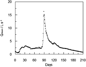Fig. 10 Recorded average daily flow (●) and predicted flow one day ahead (dot line) during the validation period for ANN₂.

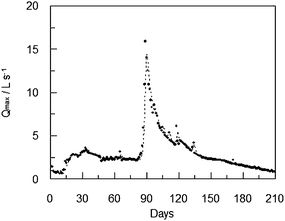Fig. 11 Maximum daily flow (●) and maximum flow predicted one day ahead (dot line) during the validation period for ANN₂.

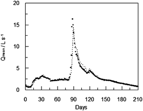Fig. 12 Recorded average daily flow (●) and predicted flow two days ahead (dot line) during the validation period for ANN₂.

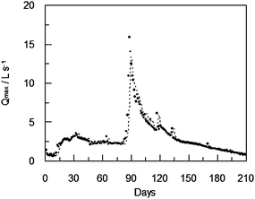Fig. 13 Maximum daily flow (●) and maximum flow predicted two days ahead (dot line) during the validation period for ANN₂.

Table 5 Parameters of fit of the forecasts, obtained for the training period (T) and ANN₂ validation (V). n is the number of values, b and a the slope and the origin of the regression line, R² the determination coefficient and RMSE the root mean squared error

	Q mean+2		Q max+2		Q mean+1		Q max+1
	T	V	T	V	T	V	T	V
n	1489	210	1489	210	1504	210	1504	210
a	0.3576	0.3797	0.3523	0.3109	0.069	0.0964	0.1135	0.0931
b	0.8763	0.8844	0.8782	0.8936	0.9732	0.9733	0.9537	0.9639
R ^2	0.963	0.929	0.955	0.903	0.991	0.974	0.983	0.962
RMSE	1.056	0.902	1.236	0.988	0.513	0.549	0.763	0.623

---

The results show that predictions obtained with ANN₂ present a real data set similar to those obtained with ANN₁, and the R² values are even slightly higher. Therefore, for predictions at 1 or 2 days of maximum or average flow it is feasible to use either ANN.

The weight of each of the variables used in the ANN₂ is shown in Table 6.

Table 6 Importance of variables for each of the developed ANNs

ANN for Qmean+2		ANN for Qmax+2
Precipitation (P)	80.0559	Precipitation (P)	72.8009
Flow at time zero (Q0)	72.8901	Flow at time zero (Q0)	72.1173
ET 0	22.9109	ET 0	14.6963

---

ANN for Qmean+1		ANN for Qmax+1
Flow at time zero (Q0)	81.9045	Flow at time zero (Q0)	75.8473
Precipitation (P)	45.8732	ET 0	47.1037
ET 0	27.8669	Precipitation (P)	20.5213

---

In analyzing the weight of the system variables (Table 6) we can observe that the key variable for the ANN2 two-day forecasts is precipitation (P), while for forecasts at one day is flow at time zero (Q₀). This change in the importance of the dependent variables can be understood as follows: the variable to present the highest incidence in the flow to a day view is the flow of the previous day, since the response to precipitation (P) presents a delay superior to a day.

Both the ANN₁ and the ANN₂ group allow calculation of Q_mean and Q_max within a day or two in an optimal manner as evidenced by the regression coefficients R² and RMSE values. At first we might think that ANN₂ will have a great advantage because the only variables used as input Q, P and ET₀ will greatly simplify the data collection effort, this, together with the fact that ET₀ can be obtained by different expressions that allow its calculation with a reduced number of variables^16–18 (and therefore its application is feasible for areas with limited climatic records), it might imply that the ANN offering greater satisfaction through usability is ANN₂. However, ANN₂ presents the problem that, faced with a lack of knowledge of one of the input variables, the weights readjustment would be less efficient than for ANN₁. This is because the new weighting readjustment would be between just two remaining input neurons. The error between the predicted and expected result would thus be of greater magnitude than for ANN₂ where adjustment would be distributed among the remaining seven neurons of the input layer.

Conclusions

ANNs used in this study have demonstrated a good capability to forecast streamflow one or two days in advance. In both cases the model efficiency, estimated by the coefficient of determination R², was higher than 0.85.

Given the behavior of ANNs and the results obtained for two or one day forecast we can say that the ANNs used to predict the flow have been demonstrated to be a valid tool for estimating the flow, both during periods of low flow and during level rise periods.

Although both flow forecasting methods can be used as their regression coefficients are high, faced with the problem of lack of input data for daily consultation the use of ANN₁ is recommended in order to reduce possible errors due to readjustment of weights.

Acknowledgements

G. Astray thanks the “Ministerio de Educación” of Spain for a FPU grant P.P. 0000 421S 14006. This research was supported by Galician Regional Government under contract PGIDIT04RFO383007PR. This research is also supported by Confederación Hidrografica del Miño-Sil.

References

1. A. Martinez de la Torre and G. Miguez-Macho, in Modelización de un escenario de futuro cambio climático en Galicia, Evidencias e Impactos del Cambio Climático en Galicia, ed. Conselleria de Medio, Ambiente e Desenvolvemento Sostible, Xunta de Galicia, Santiago de Compostela, 2009.
2. D. Xiaoqin, S. Haibin, L. Yunsheng, O. Zhu and H. Zailin, Hydrol. Processes, 2009, 23, 442–450.
3. C. Hu, Y. Hao, T. C. J. Yeh, B. Pang and Z. Wu, Hydrol. Processes, 2008, 22, 596–604.
4. I. Daliakopoulos, P. Coulibaly and I. Tsanis, J. Hydrol., 2005, 309, 229–240.
5. S. Morid, V. Smakhtin and K. Bagherzadeh, Int. J. Climatol., 2007, 27, 2103–2111.
6. F. J. Rodríguez-Rajo, G. Astray, J. A. Ferreiro-Lage, M. J. Aira, V. Jato-Rodriguez and J. C. Mejuto, Neural Networks, 2010, 23, 419–425.
7. G. Astray, F. Rodríguez-Rajo, J. A. Ferreiro-Lage, M. Fernández-González, V. Jato and J. C. Mejuto, J. Environ. Monit., 2010, 12, 2145–2152.
8. G. Astray, J. X. Castillo, J. A. Ferreiro-Lage, J. F. Gálvez and J. C. Mejuto, CyTA - Journal of Food, 2010, 8, 79–86,  DOI:10.1080/19476330903335277.
9. G. Astray, P. V. Caderno, J. A. Ferreiro-Lage, J. F. Gálvez and J. C. Mejuto, J. Chem. Eng. Data, 2010, 55(9), 3542–3547.
10. G. Astray, A. Cid, J. A. Ferreiro-Lage, J. F. Galvez, J. C. Mejuto and O. Nieto-Faza, J. Chem. Eng. Data, 2010 DOI:10.1021/je100573n.
11. G. Astray, A. Cid, O. Moldes, J. A. Ferreiro-Lage, J. F. Galvez and J. C. Mejuto, J. Chem. Eng. Data, 2010 DOI:10.1021/je100885f.
12. K. Gurney, An Introduction to Neural Networks, Routledge, London, 1997.
13. J. Hertz, R. G. Palmer and A. S. Krogh, Introduction to the theory of neural computation, Perseus Books, 1990.
14. C. V. Dawson and R. L. Wilby, Progress in Physical Geography, 2001, 25(1), 80–108.
15. E. Coppola, F. Szidarovszky, M. Poulton and E. Charles, J. Hydrol. Eng., 2003, 8(6), 348–360.
16. R. Allen Rivas and V. Caselles, Remote Sens. Environ., 2004, 93, 68–76.
17. J. D. Valiantzas, J. Hydrol., 2006, 331, 690–702.
18. R. L. Snyder, M. Orang, S. Matyac and M. E. Grismer, J. Irrig. Drain. Eng., 2005, 131, 249–253.
19. K. Ozgur, Hydrol. Processes, 2008, 22, 2449–2460.

---