Scope and limitations of principal component analysis of high resolution LC-TOF-MS data: the analysis of the chlorogenic acid fraction in green coffee beans as a case study

Abstract

Within this contribution we have analysed aqueous methanolic extracts by LC-ESI-TOF-MS of a total of 38 green bean coffee samples, which vary in terms of coffee variety and processing conditions. The LC-MS data have been analysed by principal component analysis (PCA) using different PCA processing parameters using an unsupervised non-targeted approach as well as a knowledge-based targeted approach. Furthermore, different normalisation and scaling algorithms have been applied to the PCA dataset. The scope and limitation of the various PCA parameters are discussed with respect to the ability to differentiate between samples of different groups, including different coffee varieties (Arabica or Robusta coffee) or different processing parameters and with respect to the information content of the PCA analysis on a molecular level. We could show that while distinction between different groups of samples can be successfully carried out independent of PCA parameters employed, identifying molecular markers rationalising differentiation between sample groups varies significantly between PCA parameters and requires careful choice as well as critical evaluation.

---

Introduction

All foods are functional, as they provide taste, aroma, beneficial health effects or nutritive value. All of these characteristics are ultimately linked to the molecular or chemical composition of the food material under investigation. In general, food is very complex at a molecular level containing usually thousands, in some cases tens of thousands of different chemical compounds,¹ with food processing frequently increasing this number dramatically.²

To understand parameters like sensory properties, beneficial health effects, shelf-life or any other desirable or undesirable property of a food a detailed knowledge of its composition and therefore chemistry is required and therefore becomes foremost a problem of analytical chemistry.

Many foods are as well an important commercial commodity with companies striving to maximise their profit through innovative technologies. Since the original food, e.g. a plant, cannot be patented, profits must be achieved by developing food processing techniques that result in a clear benefit to the consumer. For patent applications this benefit must usually be linked to a molecular parameter that is unique to the new process if compared to unprocessed samples. The identification of such unique molecular markers in a large set of samples if compared to another large set of samples, all containing concomitantly possibly thousands of chemical entities forms therefore a major challenge for analytical chemistry.

In the last decade statistical methods aimed at data reduction have become the method of choice to undertake such a Herculean task, with multi-variant statistical methods, in particular principal component analysis (PCA) becoming increasingly popular.³

The main philosophy of PCA is to reduce a large dataset obtained from a large number of samples, using a selected spectroscopic method, in order to extract the most important variations between the samples without loss of information. These variations are termed principal components of the samples, whereby each principal component is by definition orthogonal to the next. Ideally, variations between sample groups can be identified through the variation of a spectroscopic parameter linked to a set of unique marker molecules.

PCA is mainly employed as an unsupervised pattern recognition technique providing visualisation of a multivariate dataset, thereby revealing trends, observations and outliers. This visualisation is achieved by the transformation of variables into a covariance based coordinate system with the principal components as axis, thereby creating a two dimensional representation termed score plot, from which a grouping or pattern of sample groups can be extracted. Next to the score plot a so called loadings plot provides information about the origin of the variance, in the ideal case of LC-MS data information on a retention time (RT)–m/z pair revealing the molecular origin of the variances.

The success story of PCA has started with Nicholson work using high resolution NMR data to identify disease related biomarkers from urine or plasma samples.⁴ Using PCA NMR data of large patient groups could be successfully compared and unique biomarkers for certain diseases identified.⁴

PCA using a wide variety of analytical techniques, including NMR, IR, Raman spectroscopy, HPLC, GC, or GC-MS, has ever since been employed as an established statistical method in other areas of research including metabolomics, food analysis and medical research. Methods used vary in their practicability and information content. For example, IR or Raman analysis provides, in rapid measurements, omitting sample preparation and using portable non-expensive instrumentation, within minutes a reliable result that allows distinction between samples. However, distinction between samples is frequently based on peaks corresponding not to an individual molecular marker but rather to a large group or family of molecules present in the sample. Techniques like MS or NMR, however, require extensive sample preparation, costly sophisticated equipment resulting in satisfactory information on the structures of individual markers being present in the sample.

Due to the particular complexity of food, all of the techniques mentioned above have severe limitations with respect to type of materials amenable to investigation, resolution, sensitivity and information provided at the molecular level. Liquid chromatography coupled to mass spectrometry (LC-MS) appears to be the ideal method for PCA analysis of food material. Chromatographic separation, resulting in some degree of resolution, is coupled to high resolution MS providing a high level of sensitivity along with unsurpassed resolution. Due to molecular formula information and fragmentation data available, a multitude of molecular information on individual distinct structures contained in food responsible for variations between samples can be extracted from the analysis. The large amount of data contained in any LC-MS experiment, in particular if using tandem MS or high resolution MS, results in the fact that PCA analysis of LC-MS datasets is rare, with commercial software packages sufficiently powerful to carry out such PCA analysis only becoming available recently with few examples published.^5,6

To our knowledge no example on PCA analysis of a food material has been published yet using LC-MS data.

The aim of this contribution is to carry out a variety of PCA analysis using LC-MS data on a selected food material in order to critically evaluate the results and describe the scope and limitation of this procedure at its current level.

As a food material we have chosen green coffee bean samples for the following three reasons: firstly, we have in our research group acquired an intimate knowledge of the secondary metabolite profile and phytochemistry of this material, having over the last years identified around 100 different secondary metabolites in the green coffee bean, the large majority being chlorogenic acids.^7–9 This moderate amount of secondary metabolites ensures additionally that the large majority of signals in the LC-MS datasets can be reliably assigned to well characterised compounds. Secondly, coffee is an important commercial commodity, indeed after water and black tea the third most consumed beverage on this planet with an annual production of 4.5 Mt and a market value in excess of 5 Billion US$ of the raw material alone. Thirdly, green coffee beans are produced in two varieties Caffea arabica and Caffea canephora (otherwise known as Robusta coffee) whose distinction and adulteration form an important problem for the coffee industry. It should, however, be noted that distinction of intact green coffee beans by visual inspection is rather straightforward due to significant morphological differences between Robusta and Arabica coffee beans. Only in the case of processed coffee, either solubilised, roasted or ground a distinction based on chemical composition is required to which the methods presented here can be applied.

Supposedly high quality coffee blends consist typically of 100% Arabica coffee beans. Lower quality, cheaper blends may have some proportion of Robusta beans, or they may consist entirely of Robusta. Arabica beans produce allegedly a superior taste in the cup, being more flavourful and complex than their Robusta counterparts. Robusta beans in contrast tend to produce a less watery and bitterer brew, with a musty flavour and more body. Obviously, this difference in sensory properties could be related to the individual phytochemical profile of the two coffee varieties and could be characterised by PCA.

Metabolomics and phytochemical profiling using PCA based methods have been frequently applied to the problem of distinguishing green Arabica from Robusta coffee beans. Briandet and Downey et al. have used IR and NIR spectroscopy to study the differences between the two varieties.^10,11 NIR has been further used by Esteban-Diez and Lyman to distinguish Arabica from Robusta green coffee beans.^12,13 Wang et al. could show that as well Kona coffee could be distinguished from other varieties using FTIR spectroscopy.¹⁴ In all of this work, distinction between varieties was possible due to PCA analysis, however, due to the nature of the spectroscopic technique used, only spectroscopic bands corresponding to groups of compounds rather than individual phytochemical constituents could be identified. Rubayiza and Meurens¹⁵ could show using Raman spectroscopy that levels of the terpene kahweol and lipid content allow distinction between Arabica and Robusta green coffee beans. Materny and co-workers have demonstrated that Raman microscopy can be employed directly on a single green coffee bean to allow distinction between these two varieties, based on signals corresponding to lipids and chlorogenic acids.¹⁶ Valdenebro et al. could show that the geographic origin of green coffee beans can be identified using sterol profiles analysed by GC-MS.¹⁷ Korhonova et al. found using GC-MS based PCA that differences in volatile fractions exist between Arabica and Robusta beans.¹⁸ Mendonca and Alonso Salces were able to distinguish Arabica and Robusta green coffee beans based on PCA data using HPLC analysis of chlorogenic acid profiles.¹⁹

Materials and methods

All the chemicals (analytical grade) were purchased from Sigma-Aldrich (Bremen, Germany) and used as is. 28 different types of Arabica green coffee beans from different origins were purchased from the main supplier of coffee (Münchhausen, Bremen and supermarkets in Bremen, Germany) and 10 different types of Robusta green coffee beans were obtained as a generous offer from D.R. Wakefield & Co. Ltd., London, England.

Methanolic extract of coffee beans

10 g of each sample of different green Robusta and Arabica coffee beans was frozen using liquid nitrogen before grinding. The methanolic extract was prepared by Soxhlet extraction using aqueous methanol (70%) for 5 h. The extract was treated with Carrez reagent to precipitate colloidal material, and filtered through Machery-Nagel MN-615 folded filter paper. The methanol was removed in a rotary evaporator at reduced pressure. The aqueous residue was kept in a deep freezer at −80 °C for 1.5 h, followed by lyophilisation under 0.94 mbar for 24 h using Christ Alpha 1-4 LSC in order to remove the water from the extracted CGA (Chlorogenic acids) under most protective conditions. The extracts of CGA were stored at −20 °C until required. Before being used for LC-MS, these extracts were thawed at room temperature, dissolved in methanol (60 mg per 10 mL), and filtered through a membrane filter.

LC-TOF-MS

The LC equipment (Agilent 1100 series, Karlsruhe, Germany) comprised a binary pump, an auto sampler with a 100 µL loop, and a DAD detector with a light-pipe flow cell (recording at 320 and 254 nm and scanning from 200 to 600 nm). This was interfaced with a MicrOTOF Focus mass spectrometer (Bruker Daltonics, Bremen, Germany) fitted with an ESI source and internal calibration was achieved with 10 mL of 0.1 M sodium formate solution injected through a six port valve prior into each chromatographic run. Calibration was carried out using the enhanced quadratic mode.

HPLC

Separation was achieved on a 150 × 3 mm i.d. column containing diphenyl of 5 µm, with a 5 mm × 3 mm i.d. guard column (Varian, Darmstadt, Germany). Solvent A was water/formic acid (1000 : 0.005, v/v) and solvent B was methanol. Solvents were delivered at a total flow rate of 500 µL min⁻¹. The gradient profile was from 10% B to 70% B linearly in 60 min followed by 10 min isocratic, and a return to 10% B at 90 min and 10 min isocratic to re-equilibrate.

LC-MSⁿ

The LC equipment (Agilent 1100 series, Karlsruhe, Germany) comprised a binary pump, an auto sampler with a 100 µL loop, and a DAD detector with a light-pipe flow cell (recording at 320 and 254 nm and scanning from 200 to 600 nm). This was interfaced with an ion-trap mass spectrometer fitted with an ESI source (Bruker Daltonics HCT Ultra, Bremen, Germany), operating in full scan, auto-MSⁿ mode to obtain fragment ion m/z. As necessary, MS², MS³ and MS⁴ fragment-targeted experiments were performed to focus only on compounds producing a parent ion at m/z 397, 559, and 573. Tandem mass spectra were acquired in auto-MSⁿ mode (smart fragmentation) using a ramping of the collision energy. Maximum fragmentation amplitude was set to 1 V, starting at 30% and ending at 200%. MS operating conditions (negative mode) had been optimized using 5-caffeoylquinic acid with a capillary temperature of 365 °C, a dry gas flow rate of 10 L min⁻¹, and a nebulizer pressure of 10 psi.

Data processing

LC-MS data were processed using Data Analysis 4.0 (Bruker Daltonics, Bremen). Raw calibrated LC-MS data were further processed by Profile Analysis 2.0 (Bruker Daltonics, Bremen) and if required further processed using Origin 7.0 and Matlab. Buckets were created in an m/z value range between 300 and 900, unless stated otherwise, with a bucket size of 60 s and 1 Da. Kernels were defined as 20 s and 0.2 Da.

Results and discussion

The aim of this contribution is to assess the value of PCA analysis of LC-MS data, taking green coffee beans as an example. Detailed questions that require addressing are whether it possible to distinguish green coffee beans according to several parameters including variety of the coffee (Arabica or Robusta), geographical origin of the coffee, growth conditions (e.g. altitude) or processing conditions. How should the PCA parameters and methods be chosen in order to achieve optimal distinction? Should a distinction by PCA be possible, how can such a distinction be rationalised on a molecular level. For each PCA score plot a PCA analysis produces a so-called loading plot, in which the most important data points that are responsible for the distinction are displayed. Ideally, a PCA analysis provides a list of unique molecular markers, unique to each sample group, distinguishing two sample groups. What is the nature of these points in the loading plot? Are they molecular markers identified by PCA unique to a sample or not and if not how should PCA be carried out to identify unique molecular markers?

In order to address all of these questions we have analysed a series of aqueous methanolic extracts of 38 different green coffee bean samples by high resolution LC-ESI-TOF-MS in the negative ion mode. For the extraction process we used an optimised extraction method, if compared to previous work,¹ using a mild Soxhlet method followed by protein removal with Carrez reagent and subsequent freeze drying to yield bright yellow to orange powders. A total of 38 commercial green bean coffee samples, 10 Robusta samples and 28 Arabica samples of different geographic origins were extracted. LC-MS conditions used were as described earlier.²⁰ In addition to the high resolution mass measurements we carried out LC-ESI-tandem-MS measurements using an ion trap mass spectrometer to be able to assign individual compounds not only on the basis of retention time and high resolution m/z value, but as well to use fragmentation data for correct structure assignment. Similar to previous work, around 50–100 well resolved chromatographic peaks could be identified in each chromatogram and peaks assigned to individual distinct compounds, in the majority of chlorogenic acids. A list of selected compounds identified is given in Table 1 and structures are given in the ESI†. A typical chromatogram of a Robusta sample is shown in Fig. 1.

Table 1 Numbering, nomenclature and high resolution MS data of selected secondary metabolites identified in green bean coffee samples^22,23

No.	Name	Mol. formula	Theor. m/z (M−H)	Exp. m/z (M−H)	Error (ppm)
1	3-O-Caffeoylquinic acid	C16H18O9	353.0878	353.0881	−0.7
2	4-O-Caffeoylquinic acid	C16H18O9	353.0878	353.0884	−1.6
3	5-O-Caffeoylquinic acid	C16H18O9	353.0878	353.0892	−3.9
4	3-O-Feruloylquinic acid	C17H20O9	367.0929	367.1047	−3.4
5	4-O-Feruloylquinic acid	C17H20O9	367.0929	367.1038	−0.8
6	5-O-Feruloylquinic acid	C17H20O9	367.0929	367.1045	−2.9
7	3-O-p-Coumaroylquinic acid	C16H18O8	337.0929	337.0931	−0.5
8	4-O-p-Coumaroylquinic acid	C16H18O8	337.0929	337.0921	2.4
9	5-O-p-Coumaroylquinic acid	C16H18O8	337.0929	337.0921	2.4
10	3-O-Dimethoxycinnamoylquinic acid	C18H22O9	381.1191	381.1202	−2.8
11	4-O-Dimethoxycinnamoylquinic acid	C18H22O9	381.1191	381.1191	−2.5
12	5-O-Dimethoxycinnamoylquinic acid	C18H22O9	381.1191	381.1202	−2.8
13	3-O-Sinapoylquinic acid	C18H22O10	397.1140	397.1125	3.8
14	4-O-Sinapoylquinic acid	C18H22O10	397.1140	397.1150	−2.5
15	5-O-Sinapoylquinic acid	C18H22O10	397.1140	397.1140	−4.9
16	3,4-Di-O-caffeoylquinic acid	C25H24O12	515.1195	515.1190	1.0
17	3,5-Di-O-caffeoylquinic acid	C25H24O12	515.1195	515.1172	4.5
18	4,5-Di-O-caffeoylquinic acid	C25H24O12	515.1195	515.1170	4.9
19	3,4-Di-O-feruloylquinic acid	C27H28O12	543.1508	543.1512	−0.8
20	3,5-Di-O-feruloylquinic acid	C27H28O12	543.1508	543.1514	−1.1
21	4,5-Di-O-feruloylquinic acid	C27H28O12	543.1508	543.1539	−3.4
25	3-O-Feruloyl-4-O-caffeoylquinic acid	C26H26O12	529.1351	529.1343	1.7
26	3-O-Caffeoyl-4-O-feruloylquinic acid	C26H26O12	529.1351	529.1351	−0.1
27	3-O-Feruloyl-5-O-caffeoylquinic acid	C26H26O12	529.1351	529.1373	−4.0
28	3-O-Caffeoyl-5-O-feruloylquinic acid	C26H26O12	529.1351	529.1367	−3.0
29	4-O-Feruloyl-5-O-caffeoylquinic acid	C26H26O12	529.1351	529.1351	0.1
30	4-O-Caffeoyl-5-O-feruloylquinic acid	C26H26O12	529.1351	529.1349	0.5
31	3-O-Dimethoxycinnamoyl-4-O-caffeoylquinic acid	C27H28O12	543.1508	543.1488	3.6
32	3-O-Dimethoxycinnamoyl-5-O-caffeoylquinic acid	C27H28O12	543.1508	543.1491	3.1
33	4-O-Dimethoxycinnamoyl-5-O-caffeoylquinic acid	C27H28O12	543.1508	543.1526	−3.4
34	3-O-Dimethoxycinnamoyl-4-O-feruloylquinic acid	C27H28O12	543.1508	543.1508	−4.1
35	3-O-Dimethoxycinnamoyl-5-O-feruloylquinic acid	C27H28O12	543.1508	543.1515	−1.4
36	4-O-Dimethoxycinnamoyl-5-O-feruloylquinic acid	C27H28O12	543.1508	543.1525	−3.1
37	3-O-p-Coumaroyl-4-O-caffeoylquinic acid	C25H24O11	499.1246	499.1227	3.7
38	3-O-Caffeoyl-4-O-p-coumaroylquinic acid	C25H24O11	499.1246	499.1247	−0.2
39	3-O-p-Coumaroyl-5-O-caffeoylquinic acid	C25H24O11	499.1246	499.1248	−0.5
40	3-O-Caffeoyl-5-O-p-coumaroylquinic acid	C25H24O11	499.1246	499.1247	−0.2
41	4-O-Caffeoyl-5-O-p-coumaroylquinic acid	C25H24O11	499.1246	499.1246	−4.9
42	4-O-p-Coumaroyl-5-O-caffeoylquinic acid	C25H24O11	499.1246	499.1249	−0.6
43	3-O-p-Coumaroyl-4-O-feruloylquinic acid	C26H26O11	513.1402	513.1389	2.6
44	3-O-p-Coumaroyl-5-O-feruloylquinic acid	C26H26O11	513.1402	513.1141	−2.9
45	4-O-p-Coumaroyl-5-O-feruloylquinic acid	C26H26O11	513.1402	513.1406	−0.7
49	3-O-Sinapoyl-5-O-caffeoylquinic acid	C27H28O13	559.1457	559.1481	−4.2
50	3-O-Sinapoyl-4-O-caffeoylquinic acid	C27H28O13	559.1457	559.1472	−2.6
51	3-O-(3,5-Dihydroxy-4-methoxy)cinnamoyl-4-O-feruloylquinic acid	C27H28O13	559.1457	559.1458	−0.2
52	4-O-Sinapoyl-3-O-caffeoylquinic acid	C27H28O13	559.1457	559.1457	0.9
53	3-O-Sinapoyl-5-O-feruloylquinic acid	C28H30O13	573.1614	573.1641	−4.7
54	4-O-Sinapoyl-5-O-feruloylquinic acid	C28H30O13	573.1614	573.1599	−2.5
55	4-O-Sinapoyl-3-O-feruloylquinic acid	C28H30O13	573.1614	573.1634	−3.5
56	4-O-Trimethoxycinnamoyl-5-O-caffeoylquinic acid	C28H30O13	573.1614	573.1611	0.4
57	3-O-Trimethoxycinnamoyl-5-O-caffeoylquinic acid	C28H30O13	573.1614	573.1623	−1.7
58	3-O-Trimethoxycinnamoyl-5-O-feruloylquinic acid	C29H32O13	587.1770	587.1748	3.8
59	3-O-Trimethoxycinnamoyl-4-O-feruloylquinic acid	C29H32O13	587.1770	587.1766	0.7
60	4-O-Trimethoxycinnamoyl-5-O-feruloylquinic acid	C29H32O13	587.1770	587.1764	1.0
61	3-O-Dimethoxycinnamoyl-4-O-feruloyl-5-O-caffeoylquinic acid	C37H36O15	719.1981	719.2001	−2.7
62	3,4,5-Tri-O-caffeoylquinic acid	C34H29O15	677.1512	677.1522	−3.5
63	3,5-Di-O-caffeoyl-4-O-feruloylquinic acid	C35H31O15	691.1668	691.1647	3.1
64	3-O-Feruloyl-4,5-di-O-caffeoylquinic acid	C35H31O15	691.1668	691.1711	−6.2*
65	3,4-Di-O-caffeoyl-5-O-feruloylquinic acid	C35H31O15	691.1668	691.1647	3.1
66	3-O-Caffeoyl-4,5-di-O-feruloylquinic acid	C36H33O15	705.1825	705.1851	−3.8
67	3,4-Di-O-feruloyl-5-O-caffeoylquinic acid	C36H33O15	705.1825	705.1833	−1.1
68	3,4-Di-O-caffeoyl-5-O-sinapoylquinic acid	C36H33O16	721.1774	721.1795	−2.9
69	3-O-Sinapoyl-4,5-di-O-caffeoylquinic acid	C36H33O16	721.1774	721.1766	1.1

---

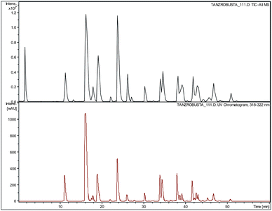Fig. 1 Representative chromatogram of green coffee extract of sample no. 33 (Tanzania Robusta): (a) TIC in negative ion mode and (b) UV-VIS chromatogram monitored at 320 nm.

PCA analysis: general remarks

For the PCA analysis, LC-ESI-TOF-MS data were employed using a commercial software package Profile Analysis 2.0 (Bruker Daltonics). LC-MS datasets are obtained as a combination of three parameters, retention time, m/z ratio and intensity. Prior to PCA these three parameters need to be reduced to two by a process referred to as bucketing: a RT–m/z value pair (termed a bucket), to which an intensity value is assigned. The simplest approach consists of a rectangular bucketing, where the buckets correspond to RT and m/z windows of adjustable size. Effects from intensities being arbitrarily cut by bucket borders are minimised by kernelising algorithms. A more advanced bucketing approach uses “compound buckets”. Here a compound finding algorithm differentiates compounds with defined chromatographic elution profiles from randomly dispersed noise in the mass spectrum. The compound information is used as an input for bucketing, thereby decreasing the number of variables to be considered in the PCA. Müller and co-workers have recently demonstrated the value of advanced bucketing by showing a significant reduction of redundant data points.⁶

A final PCA parameter worth discussing comprises normalisation and scaling routines. van den Berg has discussed this important parameter in detail and in the course of the discussion we will return to this important point on several occasions.²¹ In general, normalisation can be carried out in various ways with a “sum of all bucket intensity normalisation” being commonly employed. All MS-intensities over all buckets are summed up in all samples and normalisation will occur using these values. Details for kernelising and scaling employed are given in the Method section.

Typically, a non-targeted (unsupervised) PCA analysis is carried out, in which the full dataset is processed. Once the principal components are calculated, an inspection of the various PCA score plots allows identification of groups of samples. By inspection of the characteristics of each individual data point in the groups in the score plot a conclusion can be drawn with respect to the nature of these groups. Data points can thus be labelled according to the groups identified.

Non-targeted PCA of green coffee bean extracts

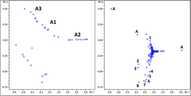
Firstly, in order to test the stability of our analytical method, three different extracts from the same green coffee bean samples were analysed in triplicate and the total of nine LC-MS datasets analysed by PCA with no variances between samples detected.

Subsequently, a non-targeted PCA analysis of all samples was carried out using rectangular bucketing and sum over bucket normalisation. An inspection of the PC1versusPC2 score plot shows that two groups of samples can be readily distinguished (see Fig. 2). The two groups of samples are Arabica and Robusta samples.

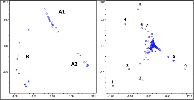Fig. 2 Score (left) and loading (right) plot of PCA analysis using regular bucketing, Robusta samples as triangles and Arabica samples as circles. Numbers in loading plot are assigned in Table 3.

In a second non-targeted PCA analysis the same dataset was analysed using advanced bucketing under identical normalisation methods. The score plot again allows differentiation between Arabica and Robusta beans (see Fig. 3). The second approach bears two advantages. Firstly, differentiation in the score plot is slightly better and secondly, the PCA dataset produced is considerably smaller requiring less computing power. Some removal of redundant information, here in particular dimeric adducts of ions could be removed from the dataset. As a further difference between the two analyses it becomes apparent that for regular bucketing distinction between Arabica and Robusta samples is achieved in PC1, whereas for the molecular feature routine distinction is achieved in PC2. An influence plot of the molecular feature PCA analysis with no data points present in the upper right quadrant of the plot is shown in the ESI†, indicating a close distance of all data points to the model, which is required in a high quality analysis.

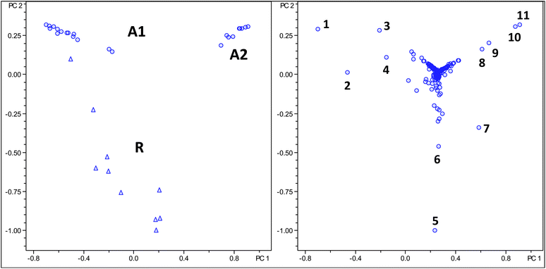Fig. 3 Score and loading plot of PCA analysis using molecular feature advanced bucketing, Robusta samples as triangles and Arabica samples as circles. Numbers in loading plot are assigned in Table 4.

At closer inspection it becomes obvious that actually three groups of samples should be recognised from the score plot. The Arabica samples cluster in two distinct groups termed A1 and A2 in both analyses. The A2 group (see Table 2) contains a larger proportion of Arabica coffees grown in Central America if compared to the A1 group. Otherwise, no obvious criteria explaining the nature of the differences between samples can be given at the current state.

Table 2 Origin, nature and grouping of green bean coffee samples analysed and included in PCA analysis

Sample no.	Origin/type	Arabica/Robusta	Group
1	Tanzania	Arabica	A1
2	Guatemala SHG	Arabica	A1
3	Peru Bio	Arabica	A1
4	Nicaragua Maragogype	Arabica	A1
5	Kenya AA	Arabica	A1
6	Athiopien Wild Forest Bio	Arabica	A1
7	Athiopien Yivgachette	Arabica	A1
8	Athiopien Mokka Sidamo 2	Arabica	A1
9	Reizaow	Arabica	A1
10	Coffeein free	Arabica	A1
11	Costarica 2	Arabica	A1
12	Brasilien 1	Arabica	A1
13	Brasilien 2	Arabica	A1
14	Maragogype	Arabica	A2
15	Malawi Pamwamba	Arabica	A2
16	Panama Boquete	Arabica	A2
17	Kenia 1	Arabica	A2
18	Honduras Bio	Arabica	A2
19	Kameruls	Arabica	A2
20	Nicaragua Mataglpa	Arabica	A2
21	Costarica 1	Arabica	A2
22	Columbia Exulso	Arabica	A2
23	Papua Neuguinea	Arabica	A3
24	Athiopien Mokka Sidamo 1	Arabica	A3
25	Costarica 3	Arabica	A3
26	Ethiopien	Arabica	A3
27	Indian Perl Mountain	Arabica	A3
28	Brazilien Santos	Arabica	A3
29	Indian 1	Robusta	R
30	India Cherry AB	Robusta	R
31	Uganda	Robusta	R
32	India Parchment	Robusta	R
33	Tanzania	Robusta	R
34	Indonesia 1	Robusta	R
35	Togo 1	Robusta	R
36	Cameron	Robusta	R
37	Indonesia 2	Robusta	R
38	India Cherry A	Robusta	R

---

A differentiation between samples from different geographic origins or growth conditions was not possible according to any score plots in any set of principal components. Examples of such plots are given in the ESI†.

PCA of LC-MS data therefore allows distinction between different coffee varieties. The next question that requires addressing is, what information was provided by the loading plot. Within the loading plot each data point corresponds to a RT–m/z pair, which is responsible for the observed variations and whose distance from the centre of the plot defines its influence on the sample grouping. From the RTs, m/z values and their corresponding tandem MS data in a separate chromatographic run, structures can be unambiguously assigned to individual data points in the loading plot.

A careful inspection of both loading plots (Fig. 2 and 3) reveals that variances between the Robusta and Arabica coffee samples are exclusively a result of differences in concentrations of regioisomeric monocaffeoyl and monoferuloylquinic acids (chlorogenic acids). It should be noted that any set of LC-MS data only provides information on relative amounts of compounds present and not on absolute concentrations, for which calibration with authentic reference materials is required. Compound assignment is given in Table 3.^22,23 From inspection of the bucket statistics in individual chromatograms it follows that concentrations for all of these compounds are higher in Robusta beans if compared to Arabica beans. This observation was already reported earlier by Materny and co-workers.¹⁶

Table 3 Assignment of data points in loading plot of green bean coffee samples using regular bucketing PCA analysis (for no. see Fig. 2)

No.	RT/s	m/z	CGA ^22,23	Abbreviation^22,23
1	1650	367	6	5-FQA
2	1410	353	2	4-CQA
3	1110	353		Unknown CQA
4	1050	353	1	3-CQA
5	1050	707		3-CQA dimer
6	1350	353	3	5-CQA
7	1590	367	4	3-FQA
8	2070	353		Unknown CQA
9	1710	353		Unknown CQA

---

Interestingly, the loading plot shows some data points with ions at m/z 353, whose tandem MS spectra identify them as previously not assigned caffeoylquinic acids, originating presumably from minor diastereoisomers of quinic acid. Additionally, the data provided here allow a rationalisation of PCA results obtained earlier by comparing different coffee varieties using low resolution spectroscopic techniques such as Raman, NIR or IR spectroscopy, clearly revealing the nature and relative concentrations of individual molecules present in the coffee samples.

Non-targeted PCA including processed coffee beans

An important aim in PCA analysis is the identification of molecular markers changing in food processing. Identification of such markers allows the rationalisation on a molecular basis of changes in sensory properties, biological effects or product consistency, which can lead to IP protection of processing parameters. For this reason we have investigated by PCA whether food processing of a green coffee bean would result in appreciable changes in the PCA scores and loading plots. As a model process we choose steaming of green coffee beans. In the coffee industry green coffee beans are frequently subjected to steam prior to roasting.^24,25 Both sensory properties and biological effects, in particular the irritation of the stomach is reduced by application of this technique, which is on a molecular level poorly understood.²⁶

Two samples of steam treated Arabica coffee were compared by PCA analysis of LC-MS data with 20 non-processed Arabica samples. Fig. 4 shows the score and loading plot clearly indicating that processed samples can be readily distinguished from non-processed samples in the PC2 dimension. The loading plot again indicates a substantial change in the chlorogenic acid profile, in particular variances in monocaffeoylquinic acids (see Table 4).^27,28

Fig. 4 Score and loading plot of PCA analysis using molecular feature advanced bucketing of processed steamed Arabica samples as circles and unprocessed Arabica samples as triangles.

Table 4 Assignment of data points in loading plot of green bean coffee samples using molecular feature bucketing PCA analysis (for no. see Fig. 3, abbreviations: C = caffeoyl, F = feruloyl, and QA = quinic acid)

No.	RT/s	m/z [M−H]	CGA ^22,23	Abbreviation^22,23
1	1050	707	1	3-CQA dimer
2	1050	353	1	3-CQA
3	1590	367	4	3-FQA
4	1350	353	3	5-CQA
5	1650	367	6	5-FQA
6	2670	367		Unknown FQA
7	1410	353	2	4-CQA
8	2070	353		Unknown CQA
9	1710	707		Unknown CQA
10	170	353		Unknown CQA
11	2250	367	5	4-FQA

---

Interestingly, the loading plot shows two data points corresponding to ions at m/z 335 (Table 5), which have been assigned on the basis of their retention time and fragmentation pattern as caffeoylquinic acid lactones, reported earlier by Farah et al. in roasted coffee.²⁹

Table 5 Assignment of data points in loading plot of green bean coffee samples comparing unprocessed and processed Arabica samples using molecular feature bucketing PCA analysis (for no. see Fig. 4, abbreviations: C = caffeoyl, F = feruloyl, QA = quinic acid, and CAL = quinic acid lactone)

No.	RT/s	m/z [M−H]	Compound
1	1095	353	3-CQA 1
2	1665	367	5-FQA 6
3	1095	707	3CQA dimer 1
4	1425	353	4-CQA 2
5	2415	515	4,5-DiCQA 5
6	1620	335	3-CAL 70
7	1695	353	Unknown CQA
8	257	683	Unassigned
9	255	341	Unassigned
10	1980	335	4-CAL 71
11	1605	367	3-FQA 4
12	1065	367	Unknown FQA

---

Targeted PCA of green coffee beans: diacyl quinic acids

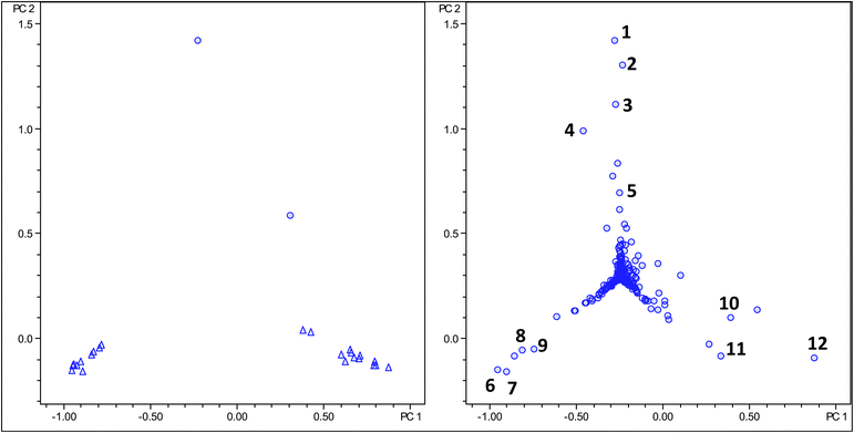
The findings provided by the loading plot are rather disappointing since the plot does not provide any new insight into the chemistry of the green coffee bean that has already been reported to contain within the extract analysed over 100 secondary metabolites. For this reason, we have carried out a second round of PCA analysis focusing on a selected class of secondary metabolitesdiacyl quinic acids.^30,31 Within this PCA analysis the m/z window within the bucket generation was reduced to values ranging from m/z 500 to 600 covering the range of all previously reported diacyl quinic acids. Müller and co-workers have termed such an approach a “knowledge based refined PCA model”.²⁷ Additionally, van den Berg has argued in favour of PCA analysis guided by prior knowledge.²⁸

The PCA results of this PCA analysis are shown in Fig. 5. Again, from the PC1versusPC2 score plot it can be seen that Robusta and Arabica samples can be readily distinguished. The Arabica samples this time show a grouping into three groups A1, A2 and A3 with the A2 group containing the same samples if compared to the previous analysis. The loading plot reveals differences in concentration of five dicaffeoylquinic acids and three caffeoyl feruloylquinic acids along with some redundant data points corresponding to dimeric ions of monocaffeoylquinic acid (Table 6). Also here, the Robusta samples all contain increased concentrations of diacyl quinic acids if compared to the Arabica samples.

Fig. 5 Score and loading plot of PCA analysis using molecular feature advanced bucketing of Arabica samples as circles and Robusta samples as triangles using a reduced m/z range window for diacyl chlorogenic acids only.

Table 6 Assignment of data points in loading plot of green bean coffee samples using molecular feature bucketing PCA analysis for reduced m/z window focusing on diacyl quinic acids exclusively (for no. see Fig. 5, abbreviations: C = caffeoyl, F = feruloyl, and QA = quinic acid)

No.	RT/s	m/z [M−H]	CGA ^22,23	Abbreviation^22,23
1	2250	515	17	3,5-DiCQA
2	2310	515	16	3,4-DiCQA
3	2490	515		Unassigned
4	2790	529	28	3C-5FQA
5	2550	515	18	4,5-DiCQA
6	2850	529	26	4F-3CQA
7	2730	529	30	4C-5FQA
8	2370	515		Unassigned

---

Targeted PCA of green coffee beans: unique chlorogenic acids

In previous work, based on the analysis of only ten samples, we have suggested that Robusta coffee beans contain a series of unique chlorogenic acids not present in Arabica coffee, including sinapoylquinic acids, trimethoxycinnamoyl quinic acids and triacyl quinic acids.^22,23 From the previous PCA results it became obvious that none of these potentially unique molecular markers could be identified as important data points in the loading plot. For this reason we carried out two further knowledge based targeted PCA analyses focusing on these compounds. A first analysis comprised a m/z window of 370 to 500 including monoacyl quinic acids (Fig. 6 and Table 7) and a second analysis comprising an m/z window of 600–700 including triacyl quinic acids (data not shown).^22,23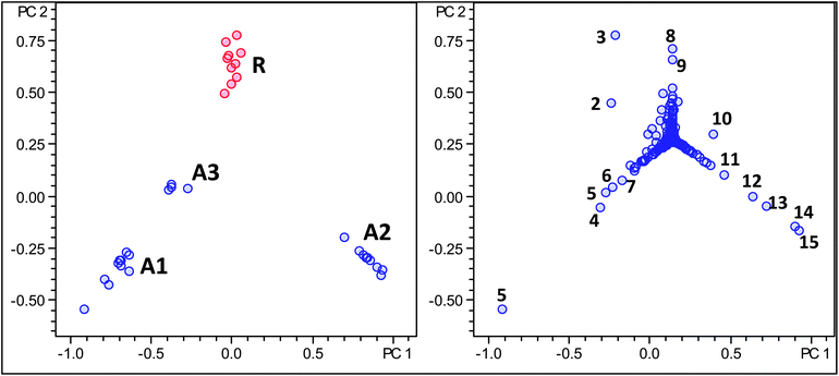

Fig. 6 Score and loading plot of PCA analysis using molecular feature advanced bucketing of Arabica samples in blue and Robusta samples in red using a reduced m/z range window for minor metabolites (m/z 370–500 and 600–700) only.

Table 7 Assignment of data points in loading plot of green bean coffee samples using molecular feature bucketing PCA analysis using a reduced m/z range window for minor metabolites (m/z 370–500 and 600–700) only (for no. see Fig. 6)

No.	RT/s	m/z [M−H]	Compound
1	1655	377
2	135	387
3	165	405
4	2025	481
5	735	375	Caffeoyl conjugate
6	135	405
7	135	379
8	795	375	Caffeoyl conjugate
9	2985	379
10	1425	375	Caffeoyl conjugate
11	1725	375	Caffeoyl conjugate
12	375	405
13	255	387
14	255	455
15	255	377

---

An influence plot (Fig. 7) of the molecular feature PCA analysis with no data points present in the upper right quadrant of the plot, indicating a close distance of all data points to the model, which is required in a high quality analysis.

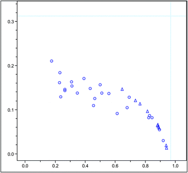Fig. 7 Influence plot of PCA analysis using molecular feature advanced bucketing of Arabica samples as circles and Robusta samples as triangles using a reduced m/z range window for minor metabolites (m/z 370–500 and 600–700) only.

The results here, using a larger sample group and a more advanced statistical tool, confirm our initial hypothesis that sinapoylquinic acids, trimethoxycinnamoyl quinic acids and triacyl quinic acids are indeed unique phytochemical markers for Robusta coffee, absent in all Arabica samples investigated. The use of these markers might be helpful in differentiating between roasted Arabica and with Robusta adulterated coffee samples.

In both cases, Arabica and Robusta coffee varieties could be distinguished based solely on secondary metabolites observed in this reduced m/z window. Indeed, as postulated, unique markers for Robusta coffee could be identified using this approach comprising sinapoylquinic acids.

This result clearly demonstrates that with a priori knowledge about sample composition unique markers allowing distinction between samples can be identified.

Scaling and normalisation

In the previous PCA analysis it became obvious that using an unsupervised non-targeted approach loading plots only revealed differentiation between groups of samples based on differences in concentration of major secondary metabolites characterised by high signal intensity in the total ion chromatograms (TICs). Only with a selection of a manually selected reduced m/z window, based on preceding knowledge of the samples was it possible to identify unique molecular markers present in only one group of samples. Based on the earlier arguments this identification of unique molecular markers is paramount for IP protection of food processing parameters and is certainly more suited for sample discrimination if compared to variances based on relative concentrations of major components. We reasoned that the failure of previous PCA analysis to identify such unique markers was based on the normalisation and scaling algorithms employed in the analysis. van den Berg and co-workers have recently highlighted and discussed the influence of scaling and normalisation algorithms on the outcome of a PCA analysis of GC-MS datasets.²⁸

For this reason, we have investigated the outcome of a PCA analysis of LC-MS data using various scaling and normalisation algorithms. It should be noted that in order to achieve similar results alternative mathematical data treatment routines such as data transformation could achieve similar results.^18,28 For example the “log ratio” transformation has been previously employed to transform heteroscedastic datasets.¹⁸

As scaling and normalisation procedures we have chosen Pareto scaling, variance scaling, and unit variance scaling. Pareto scaling reduces the relative importance of large values, while keeping the data structure largely intact.²⁸ In variance and unit variance scaling (often referred to as autoscaling) the standard deviation is used as the scaling factor resulting in an outcome, in which all metabolites are equally important, however, inflating the measurement errors.²⁸ For the latter poor differentiation for Arabicaversus Robusta coffee was observed, however, in the loading plot indeed minor components could be as expected located as important parameters responsible for variances.

Using Pareto scaling, Arabica and Robusta coffees could be readily distinguished in the PC1versusPC2 score plot (Fig. 8). The loading plot revealed next to major components, such as monocaffeoylquinic acids, a series of minor components including triacyl quinic acids, unique secondary metabolites of Robusta coffee (Table 8).

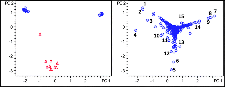Fig. 8 Score and loading plot of PCA analysis using molecular feature advanced bucketing, Robusta samples as triangles and Arabica samples as circles using Pareto scaling.

Table 8 Assignment of data points in loading plot of green bean coffee samples using molecular feature bucketing PCA analysis using Pareto scaling (for no. see Fig. 8, abbreviations: C = caffeoyl, F = feruloyl, S = sinapoyl, T = trimethoxycinnamoyl, and QA = quinic acid)

No.	RT/s	m/z [M−H]	Comp. no	Abbreviation
1	1410	353	2	4-CQA
2	1605	367	4	3-FQA
3	1790	397	15	5-SQA
4	1065	353	1	3-CQA
5	1635	367	6	5-FQA
6	2090	397	14	4-SQA
7	2265	367	5	4-FQA
8	3395	573	57	5C-3TQA
9	2470	677	62	3,4,5-TriCQA
10	2295	515	16	3,4-DiCQA
11	2250	515	17	3,5-DiCQA
12	2570	515	18	4,5-DiCQA
13	2725	529	26	4C, 5FQA
14	3125	691	65	3,5-DiC, 4FQA
15	3360	705	67	3,4-DiF, 5CQA

---

Conclusion

In conclusion we have analysed aqueous methanolic extracts of a total of 38 green bean coffee samples, containing a moderate number of around 100 well characterised secondary metabolites, which vary in terms of coffee variety and processing conditions by LC-ESI-TOF-MS. The LC-MS data have been analysed by principal component analysis (PCA) using different PCA processing parameters using an unsupervised non-targeted approach as well as a knowledge based targeted approach. Furthermore, different normalisation and scaling algorithms have been applied to the PCA dataset. The scope and limitation of the various PCA parameters have been discussed with respect to the ability to differentiate between samples of different groups, including different coffee varieties (Arabica or Robusta coffee) or different processing parameters and with respect to the information content of the PCA analysis on a molecular basis. We could show that while distinction between different groups of samples can be successfully carried out generally independent of PCA parameters, identification of molecular markers that rationalise differentiation between sample groups varies significantly between PCA parameters. In non-targeted approaches mainly major metabolites present in significant concentrations appear in the loading plot and explain variances. Unique molecular markers can only be identified in a targeted knowledge based approach, in which PCA analysis is carried out in a selected m/z window or by applying scaling routines such as Pareto scaling. Additionally, we have rationalised previous PCA work on green coffee beans using low resolution spectroscopic techniques on a molecular level providing unambiguous structure assignment for compounds responsible for variances. We have also confirmed the use of a series of chlorogenic acids as unique biomarker for Robusta coffee.

This paper provides a demonstration of the capabilities of PCA analysis using high resolution LC-MS data, pointing out some potential pitfalls. It represents a first systematic study of PCA methodology using LC-MS data in food chemistry facilitating future use of this powerful data reduction methodology in all areas of food chemistry.^3,4

References

1. J. W. Drynan, M. N. Clifford, J. Obuchowicz and N. Kuhnert, Nat. Prod. Rep., 2010, 27, 417–462.
2. R. Jaiswal, T. Sovdat, F. Vivan and N. Kuhnert, J. Agric. Food Chem., 2010, 58, 5471–5484.
3. S. Wold, K. Esbensen and P. Geladi, Chemom. Intell. Lab. Syst., 1987, 2, 37–52.
4. J. K. Nicholson, J. C. Lindon and E. Holmes, Xenobiotica, 1999, 29, 1181–1189.
5. D. Krug, G. Zurek, B. Schneider, C. Bassmann and R. Müller, LC·GC Eur., 2007, 41–42.
6. D. Krug, G. Zurek, B. Schneider, R. Garcia and R. Müller, Anal. Chim. Acta, 2008, 624, 97–106.
7. M. N. Clifford, K. L. Johnston, S. Knight and N. Kuhnert, J. Agric. Food Chem., 2003, 51, 2900–2911.
8. M. N. Clifford, S. Knight, B. Surucu and N. Kuhnert, J. Agric. Food Chem., 2006, 54, 1957–1969.
9. M. N. Clifford, S. Marks, S. Knight and N. Kuhnert, J. Agric. Food Chem., 2006, 54, 4095–4101.
10. R. Briandet, E. K. Kemsley and R. H. Wilson, J. Agric. Food Chem., 1996, 44, 170–174.
11. G. Downey, R. Briandet, R. H. Wilson and E. K. Kemsley, J. Agric. Food Chem., 1997, 45, 4357–4361.
12. D. J. Lyman, R. Benck, S. Dell, S. Merle and J. Murray-Wijelath, J. Agric. Food Chem., 2003, 51, 3268–3272.
13. I. Esteban-Diez, J. M. Gonzalez-Saiz, C. Saenz-Gonzalez and C. Pizarro, Talanta, 2007, 71, 221–229.
14. J. Wang, S. Jun, H. C. Bittenbender, L. Gautz and Q. X. Li, J. Food Sci., 2009, 74, C385–C391.
15. A. B. Rubayiza and M. Meurens, J. Agric. Food Chem., 2005, 53, 4654–4659.
16. R. M. El-Abassy, P. Donfack and A. Materny, Food Chem., in press.
17. M. S. Valdenebro, M. Leon-Camacho, F. Pablos, A. G. Gonzalez and M. J. Martin, Analyst, 1999, 124, 999–1002.
18. M. Korhonova, K. Hron, D. Klimcikova, L. Mueller, P. Bednar and P. Bartak, Talanta, 2009, 80, 710–715.
19. R. M. Alonso-Salces, F. Serra, F. Reniero and K. Heberger, J. Agric. Food. Chem., 2009, 57, 4224–4235.
20. N. Kuhnert, R. Jaiswal, M. F. Matei, T. Sovdat and S. Deshpande, Rapid Commun. Mass Spectrom., 2010, 24, 1575–1582.
21. R. A. van den Berg, H. C. J. Hoefsloot, J. A. Westerhuis, A. K. Smilde and M. J. van der Werf, BMC Genomics, 2006, 7, 142–146.
22. R. Jaiswal and N. Kuhnert, Rapid Commun. Mass Spectrom., 2010, 24, 2283–2294.
23. R. Jaiswal, M. A. Patras, P. J. Eravuchira and N. Kuhnert, J. Agric. Food Chem., 2010, 58, 8722–8737.
24. J. Baggenstoss, L. Poisson, R. Kaegi, R. Perren and F. Eschert, J. Agric. Food Chem., 2008, 56, 5847–5851.
25. S. Gal, P. Windemann and E. Baumgartner, Chimia, 1976, 30, 68–71.
26. I. M. Kamal, V. Sobolik, M. Kristiawan, S. M. Mounir and K. Allaf, Innovative Food Sci. Emerging Technol., 2008, 9, 534–541.
27. M. N. Clifford, W. Zheng and N. Kuhnert, Phytochem. Anal., 2006, 17, 384–393.
28. R. A. van den Berg, C. M. Rubingh, J. A. Westerhuis, M. J. van der Werf and A. K. Smilde, Anal. Chim. Acta, 2009, 651, 173–181.
29. D. Perrone, A. Farah, C. M. Donangelo, T. de Paulis and P. R. Martin, Food Chem., 2008, 106, 859–867.
30. M. N. Clifford, J. Kirkpatrick, N. Kuhnert, H. Roozendaal and P. R. Salgado, Food Chem., 2008, 106, 379–385.
31. M. N. Clifford, W. G. Wu and N. Kuhnert, Food Chem., 2006, 95, 574–578.

---

Footnote

† Electronic supplementary information (ESI) available: structures of compounds in Table 1, additional score and loading plots. See DOI: 10.1039/c0ay00512f

---