Mutual interference problems in the simultaneous voltammetric determination of trace total mercury(II) in presence of copper(II) at gold electrode. Applications to environmental matrices

Abstract

The present work describes and discusses the possible interference problems in the voltammetric determination of ultra-trace concentrations of Hg(II) in the presence of Cu(II) at a gold electrode, using three different supporting electrolytes: 0.1 mol L⁻¹ HClO₄, 0.01 mol L⁻¹ EDTA-Na₂ + 0.06 mol L⁻¹ NaCl + 2.0 mol L⁻¹ HClO₄ and 0.1 mol L⁻¹ KSCN + 0.001 mol L⁻¹ HClO₄. The square wave anodic stripping voltammetric (SWASV) measurements were carried out using a conventional three-electrode cell, with a gold electrode (GE) as the working electrode, and platinum wire and Ag|AgCl|KCl_sat as auxiliary and reference electrodes, respectively. The analytical procedure was validated by the analysis of the standard reference materials Estuarine Sediment BCR-CRM 277, River Sediment BCR-CRM 320 and Mercury in Water NIST-SRM 1641d. In the presence of reciprocal interference, the standard addition method considerably improved the resolution of the voltammetric technique even in the case of very high concentration ratios of both metals. The analytical procedure was transferred and applied to sediments and sea waters sampled in a lagoon ecosystem connected to the Adriatic Sea and located in proximity to the Ravenna area (Italy).

---

1. Introduction

Mercury is a highly toxic element^1,2 which can be accumulated in the food chain mainly in the form of methyl-mercury, since inorganic mercury is easily methylated by biological processes.³ Considering that every year many tons of mercury are released into the environment as a consequence of human activity, it is evident that this element should be carefully monitored in order to assess the existence of possible risks to man and wildlife.⁴ Such mercury contamination of the environment has thus promoted an intensive search for methods aimed at the determination of this metal.

The literature reports several methods for mercury determination at low concentrations in all the matrices of interest: clinical,⁵ biological^6,7 and environmental.^8,9 These methods are based on a wide range of techniques, including inductively coupled plasma mass spectrometry,^10,11 liquid and gas chromatography,^12,13 neutron activation analysis,¹⁴ nuclear magnetic resonance,¹⁵ electrothermal atomisation atomic absorption spectrometry,¹⁶ cold vapour atomic absorption spectrometry,^17,18 atomic fluorescence spectrometry¹⁹ and also, less recently, potentiometric stripping analysis.^20,21

Voltammetric measurements are more rarely employed even though voltammetry may be a good alternative to spectroscopy, since it allows for determination without the use of very expensive equipment. Such a technique employs gold,^22–24 glassy carbon²⁵ and platinum²⁶ electrodes, generally using acidic media as the supporting electrolyte. Recently, modified solid electrodes^27,28 and ultra-microelectrode arrays²⁹ have also been successfully employed for the voltammetric determination of Hg(II).

The problem relevant to the interference from other metals is rarely highlighted enough,^{22,23,30–32} and only qualitative information is given, without proposing solutions. Evidently, this problem arises in the case of multi-component determinations, when the voltammetric signals overlap, owing to neighbouring elements having very close peak potentials and very high concentration ratios. The present work suggests a simple and quick procedure to show that voltammetric techniques, if appropriately coupled to the standard addition method,³³ allow for the resolution of highly overlapping voltammetric signals. Such an analytical procedure, set up for the first time in the case of Hg(II) determination at a gold electrode, especially if applied to samples of great interest, e.g. environmental matrices, may certainly encourage the employment of the same voltammetric methods, instead of, for example, spectroscopic techniques.

2. Experimental

2.1. Apparatus

A Multipolarograph AMEL (Milan, Italy) Mod. 433 was employed for all the voltammetric scans, using a conventional three electrode measuring cell: a gold electrode (GE) (surface area: 0.785 mm²) as the working electrode, activated following the procedure suggested by Bonfil et al.,²² and an Ag|AgCl|KCl_sat electrode and a platinum wire as the reference and auxiliary electrodes, respectively.

The experimental conditions are reported in Table 1. When a gold electrode is employed, a problem is always present linked to the presence of anions in solution. In fact, anions are known to adsorb strongly on gold surfaces,³⁴ and this adsorption is dependent on the potential of the electrode and on the nature of the anion. According to Salaun and van den Berg,²³ to minimize the excessive adsorption effect, in order to have higher voltammetric peaks and a flatter voltammetric baseline, a negative potential of −0.8 V/Ag|AgCl|KCl_sat was applied between the deposition and the stripping steps. It has been shown that, at this potential, Cl⁻, Br⁻, I⁻ and SO₄²⁻ do not adsorb on the gold electrode.^34,35

Table 1 Instrumental parameters for the determination of Hg(II) and Cu(II), by Square Wave Anodic Stripping Voltammetry (SWASV)^a

	0.1 mol L^−1 HClO4	0.01 mol L^−1 EDTA-Na2 + 0.06 mol L^−1 NaCl + 2.0 mol L^−1 HClO4	0.1 mol L^−1 KSCN + 0.001 mol L^−1 HClO4
a E i: initial potential (V/Ag|AgCl|KClsat); Ed: deposition potential (V/Ag|AgCl|KClsat); Edes: desorption potential (V/Ag|AgCl|KClsat); Ef: final potential (V/Ag|AgCl|KClsat); td: electrodeposition time (s); tdes: desorption time (s); tr: delay time before the potential sweep (s); dE/dt: potential scan rate (mV s^−1); ΔE: step amplitude (mV); τ: sampling time (s); ν: wave period (s); η: wave increment (mV); r: stirring rate (r.p.m.).
E i	+0.150	+0.150	−0.600
E d	+0.150	+0.150	−0.600
E des	−0.800	−0.800	−0.800
E f	+0.800	+0.800	+0.100
t d	240	240	240
t des	30	30	—
t r	10	10	10
dE/dt	100	100	100
ΔE	50	50	50
τ	0.010	0.010	0.010
ν	0.100	0.100	0.100
η	10	10	10
r	600	600	600

---

For all the supporting electrolytes, experimental data show that, applying a desorption potential at −0.8 V/Ag|AgCl|KCl_sat, Hg(II) and Cu(II) maintain an excellent stability of the voltammetric signal (rsd < 5% for peak height and potential over a period of 2 h of continuous measurements). Also, the effect due to possible EDTA-Na₂ and SCN⁻ adsorption, even if present, was eliminated.

Before the measurements, to avoid accidental contamination, the Teflon voltammetric cell was rinsed with suprapure concentrated 1 : 1 HNO₃ and then many times with Milli-Q water. The solutions were thermostated at 20 ± 0.5 °C and deaerated with Milli-Q water-saturated pure nitrogen for 5 min prior to analysis, while a nitrogen blanket was maintained above the solutions during the experiments. The solutions were stirred with a Teflon-coated magnetic stirring bar in the purge step.

The atomic absorption spectrometry Hg(II) measurements were performed in the recirculation mode³⁶ employing stannous chloride as a reducing agent and using a Perkin-Elmer Mod. Zeeman 5100 PC Atomic Absorption Spectrometer, equipped with a Zeeman background corrector. The absorption wavelength was fixed at 253.7 nm and the spectral bandwidth at 0.7 nm. The spectroscopic experimental conditions relevant to Cu(II) are the following. Wavelength (nm): 324.8; slit (nm): 0.7; drying T/°C: 110; charring T/°C: 1350; atomization T/°C: 2500; matrix modifiers: 0.015 mg Pd + 0.03 mg Mg(NO₃)₂. Single-element Intensitron hollow-cathode lamps were used.

2.2. Reagents and reference solutions

All acids and chemicals were suprapure grade (Merck, Germany). Acidic stock metal solutions (1000 mg L⁻¹, Merck, Darmstadt, Germany) were employed in the preparation of reference solutions at varying concentrations for each element, using, for dilution, water demineralized through a Milli-Q system.

The three supporting electrolytes employed were 0.1 mol L⁻¹ HClO₄, 0.01 mol L⁻¹ EDTA-Na₂ + 0.06 mol L⁻¹ NaCl + 2.0 mol L⁻¹ HClO₄ and 0.1 mol L⁻¹ KSCN + 0.001 mol L⁻¹ HClO₄.

A special treatment was applied to potassium dichromate to render it virtually mercury-free: the salt was kept heated at 350 °C for 4 days, then the temperature was raised to 410 °C and the mass kept melted for 24 h. The solidified salt was granulated and homogenized by corundum ball-milling.

The reducing agent SnCl₂·2H₂O was dissolved in 10% (w/w) H₂SO₄ to give a 25% (w/w) solution which was bubbled with N₂ for 20 min to strip away any residual Hg and O₂.

Estuarine Sediment BCR-CRM 277, River Sediment BCR-CRM 320 and Mercury in Water NIST-SRM 1641d. were employed as standard reference materials for optimising and setting up the analytical procedure.

2.3. Sampling and sample preparation

a) Sediments. Sampling was performed by means of a plexiglass device: single carrots (section: 69.7 cm², height: 10 cm) were drawn out and put in polyethylene bottles, previously washed with a solution of 20% suprapure HNO₃ for 72 h and finally rinsed many times with Milli-Q deionised water. The sedimentary texture shows that clay and silt are the predominant size fraction (higher than 79% in all cases).

The samples, once dried at 45 °C for 96 h, were passed through a 10 mesh inox sieve, to eliminate coarse material, powdered by means of a corundum ball mill, and passed through a 150 mesh inox sieve. Finally, they were dried at 50 °C for 48 h prior to the sample preparation.

To solubilise the sediments, HNO₃-HCl acidic mixture has been employed. Approximately 1.0 g of sediments, accurately weighed, was placed in a Pyrex digestion tube calibrated at 25 mL and connected with a Vigreux column condenser together with 3 mL 69% (w/w) HNO₃ + 2 mL 37% (w/w) HCl. The tube was inserted into the cold home-made block digester, raising the temperature gradually up to 130–150 °C, and keeping this temperature for the whole time of mineralisation (2 h). After cooling, the digest was filtered through Whatman N. 541 filter paper, evaporated to dryness and the soluble salts dissolved in 50 mL of each supporting electrolyte under study.

b) Sea water. Sea water samples were taken with a portable suction pump made of stainless steel and pyrex glass, neither of which would yield contamination with all the elements to be determined. Model experiments exactly simulating the sampling procedure were performed with artificial fresh and sea water, to verify that the samples would not be contaminated by the sampling device. The concentrations of both analytes in these artificial samples were found to be lower than the relevant limits of detection.

Water samples were immediately filtered on the spot through 0.22 μm membranes and transferred into polyethylene bottles, previously soaked in 1 : 1 nitric acid for 48 h and rinsed many times with deionised water (Milli-Q). The samples were cooled to 4 °C for transport, stored at this temperature and analysed within 72 h. 0.1 mol L⁻¹ HClO₄, 0.01 mol L⁻¹ EDTA-Na₂ + 0.06 mol L⁻¹ NaCl + 2.0 mol L⁻¹ HClO₄ and 0.1 mol L⁻¹ KSCN + 0.001 mol L⁻¹ HClO₄ in sea water samples were employed as solutions for the voltammetric scans.

For the spectroscopic determination of Hg(II) in sediments and sea water, a different sample preparation procedure was followed.³⁷

a. Sediments. Approximately 1.0 g of sediment, accurately weighed, was placed in a digestion tube together with 1.2 g K₂Cr₂O₇ and 20 mL H₂O. A condenser was connected to the digestion tube and 20 mL H₂SO₄ was slowly added. The digestion tube was transferred to the hot block preheated at 180 °C, and the digestion was allowed to proceed for 60 min to completion. After cooling at room temperature, the condenser was removed, rinsed with three 5 mL portions of H₂O and the washings were added to the digested matter. The open digestion tube, without the condenser, was replaced on the hot-block for a further 30 min boiling span. Finally, after cooling, the digested solution was diluted to 100 mL.
b. Sea water. In the case of sea water, 1 g L⁻¹ of K₂Cr₂O₇ was added to the water samples before their determination by CV-AAS (Cold Vapour Atomic Absorption Spectrometry), using SnCl₂ as a reducing agent.

3. Results and discussion

At first, the analytical procedure was set up in aqueous reference solutions, then successively verified by the analysis of standard reference materials and finally applied to real samples.

3.1. Aqueous reference solutions

The choice of the three supporting electrolytes (0.1 mol L⁻¹ HClO₄, 0.01 mol L⁻¹ EDTA-Na₂ + 0.06 mol L⁻¹ NaCl + 2.0 mol L⁻¹ HClO₄ and 0.1 mol L⁻¹ KSCN + 0.001 mol L⁻¹ HClO₄) is suggested by two factors: a) the anodic stripping voltammetric determination of Hg(II) is predominantly carried out in acidic medium, and b) it is well known that EDTA forms complexes with Hg(II) and Cu(II), as does SCN⁻, and that the latter forms much more stable complexes with Hg(II) than with Cu(II).

Therefore, HClO₄ may be considered the main medium. Moreover, the complexes of the two elements generally show wider voltammetric peak potential differences in comparison with the single elements. For this reason, the addition of EDTA-Na₂ and SCN⁻ seemed suitable to obtain wider peak potential differences, and consequently a better resolution between the Hg(II) and Cu(II) voltammetric signals, so minimizing the interference problem. In reality, the EDTA-Na₂ and SCN⁻ additions increased the non-interference concentration ratio intervals (see section 3.1.1 “Interference Problems”), even if, unfortunately, not in a marked and considerable way, as expected.

A preliminary study was carried out employing aqueous reference solutions for the voltammetric determinations of Hg(II). The blank concentrations for all the elements, Hg(II) and eventual interfering metals, were lower than the respective limits of detection. Using the instrumental experimental conditions given in Table 1, the analytical calibration functions of each individual element were determined in the aqueous reference solutions. In the range of concentrations investigated a linear relationship between i_p and metal concentration was found for each single element. In all cases the correlation coefficients were good (r² > 0.9990).

Table 2 reports the experimental Hg(II) and Cu(II) peak potentials in each supporting electrolyte.

Table 2 Experimental peak potentials (E_p, V, Ag|AgCl|KCl_sat) and half peak width w_1/2 (mV) in the aqueous reference solutions and in the standard reference material solutions. The determined values are the mean of 5 independent determinations ± confidence interval at 95% probability level

		Experimental peak potential		Half peak width w1/2
		Hg(II)	Cu(II)	Hg(II)	Cu(II)
0.1 mol L^−1 HClO4	a	0.56 ± 0.02	0.41 ± 0.01	56 ± 1	55 ± 2
0.01 mol L^−1 EDTA-Na2 + 0.06 mol L^−1 NaCl + 2.0 mol L^−1 HClO4	b	0.53 ± 0.01	0.37 ± 0.01	47 ± 1	49 ± 1
0.1 mol L^−1 KSCN + 0.001 mol L^−1 HClO4	c	−0.19 ± 0.01	−0.37 ± 0.02	69 ± 2	77 ± 2
Estuarine Sediment BCR-CRM 277	a	0.58 ± 0.01	0.44 ± 0.02	57 ± 2	58 ± 2
	b	0.55 ± 0.02	0.39 ± 0.01	46 ± 1	48 ± 2
	c	−0.19 ± 0.01	−0.34 ± 0.02	73 ± 3	80 ± 3
River Sediment BCR-CRM 320	a	0.59 ± 0.01	0.44 ± 0.01	59 ± 2	58 ± 2
	b	0.56 ± 0.01	0.40 ± 0.01	48 ± 1	50 ± 1
	c	−0.21 ± 0.02	−0.37 ± 0.02	72 ± 3	79 ± 3
Mercury in Water, NIST-SRM 1641d	a	0.57 ± 0.01	0.42 ± 0.01	57 ± 1	60 ± 3
	b	0.51 ± 0.01	0.37 ± 0.01	46 ± 1	47 ± 2
	c	−0.22 ± 0.02	−0.37 ± 0.02	70 ± 3	75 ± 2

---

3.1.1. Interference problems. Often, in the commonly used supporting electrolytes, the reduction peak potentials of each metal are very close and thus the simultaneous voltammetric determination of neighbouring elements can be hindered. In the case of Hg(II) determination, the most important interferent, only qualitatively investigated,^{22,23,30–32} is Cu(II).

The voltammetric interference between two neighbouring metals is strictly linked to two parameters: 1) the metal concentration ratio, and 2) the degree of reversibility of the element electrodic process. If the former depends exclusively on the matrix element composition, the latter, as is well known, influences the half peak width w_1/2.^38,39 The lower the reversibility of the electrodic process, the higher the w_1/2, and consequently the higher the possibility of peak overlapping, if the voltammetric peaks prove not to be separated enough. Generally, reversible electrodic processes should have w_1/2 values, independent of concentration, equal to 90.6/n mV at 20 °C, where n is the number of electrons involved in the electrodic process.

Table 2 reports the Hg(II) and Cu(II) w_1/2 data relevant either to the aqueous reference solutions or to the standard reference materials. Considering the reversibility of the electrodic process, even if the w_1/2 data give only qualitative information, 0.01 mol L⁻¹ EDTA-Na₂ + 0.06 mol L⁻¹ NaCl + 2.0 mol L⁻¹ HClO₄ seems to be the best supporting electrolyte for Hg(II) and Cu(II). In fact, in this supporting electrolyte, these metals present w_1/2 data close to theoretical values.

Some works^22,30 affirm that Cu(II) does not seem to interfere in the Hg(II) determination at the GE for concentrations lower than 10 mg L⁻¹. On the contrary, in my opinion, the mutual interference is due exclusively to the concentration ratio between Hg(II) and Cu(II). In fact, both metals are shown to have reversible electrodic processes at the gold electrode (w_1/2 ≅ 45 mV, Table 2), and, consequently, well defined peaks, also at ultra-trace concentration levels.

The possible interference problems of Hg(II)–Cu(II), due to the peak overlapping owing to the closeness between the respective peak potentials, were analysed for all the supporting electrolytes under study, with the peak potential differences as follows:

a) 0.1 mol L⁻¹ HClO₄: ΔE_pHg–Cu = 150 mV;

b) 0.01 mol L⁻¹ EDTA-Na₂ + 0.06 mol L⁻¹ NaCl + 2.0 mol L⁻¹ HClO₄: ΔE_pHg–Cu = 160 mV;

c) 0.1 mol L⁻¹ KSCN + 0.001 mol L⁻¹ HClO₄: ΔE_pHg–Cu = 180 mV

In order to establish the degree of interference, and consequently the element concentration ratios within which it is possible to determine each metal, the simultaneous determination of both the interfering metals was studied in a wide range of concentration ratios, in the concentration range corresponding to the respective calibration functions in all the supporting electrolytes under study.

Although the standard addition method has already been applied²² to determine Hg(II), in the present work this method is employed to solve the problem of Hg(II) and Cu(II) determination in the presence of very high mutual signal interference. Then, following the standard addition method previously described for mercury electrodes,³³ but not yet applied to solid electrodes and in particular to the gold electrode, standard additions of the interfering element were added to a fixed concentration of the element of interest, i.e. Hg(II), in such a way as to change their concentration ratios. The peak current values of each element in the various mixtures were compared to those calculated by using the respective analytical calibration function. The errors of these data, as a function of the concentration ratios, were calculated.

If a maximum experimental error of 5% is fixed, at the 95% confidence level, the concentration ratios (concentration expressed in μg L⁻¹), within which Hg(II) and Cu(II) may be determined, are as follows:

a) 0.1 mol L⁻¹ HClO₄: 177 : 1 > c_Cu : c_Hg > 1 : 196;

b) 0.01 mol L⁻¹ EDTA-Na₂ + 0.06 mol L⁻¹ NaCl + 2.0 mol L⁻¹ HClO₄: 223 : 1 > c_Cu : c_Hg > 1 : 249;

c) 0.1 mol L⁻¹ KSCN + 0.001 mol L⁻¹ HClO₄: 209 : 1 > c_Cu : c_Hg > 1 : 221

Fig. 1 shows the errors relevant to the Hg(II)–Cu(II) couple in each supporting electrolyte. The zero value corresponds simultaneously to c_Hg = 0 in the case of concentration ratio c_Hg : c_Cu and c_Cu = 0 in the case of concentration ratio c_Cu : c_Hg. Moreover, it is important to highlight that the above non-interference concentration ratio intervals a), b) and c) are independent of the single Hg(II) and Cu(II) concentrations, and consequently the determination of each element is always possible: it is sufficient that, for each supporting electrolyte, the Hg(II)–Cu(II) concentration ratios are within the above-cited intervals.

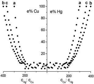Fig. 1 Relationship between the Hg(II)–Cu(II) concentration ratios and the relative errors in the determination of the element present in the mixture at lower concentration. Supporting electrolytes: a) 0.1 mol L⁻¹ HClO₄, b) 0.01 mol L⁻¹ EDTA-Na₂ + 0.06 mol L⁻¹ NaCl + 2.0 mol L⁻¹ HClO₄, c) 0.1 mol L⁻¹ KSCN + 0.001 mol L⁻¹ HClO₄. Values between which the concentrations (μg L⁻¹) of Hg(II) and Cu(II) are included: 0.5–2 × 10² (a and b), 3.5–1.4 × 10³ (c).

Obviously, the interesting aspect of the analytical procedure proposed is the possibility of determining the metal with the lower concentration and an unfavourable concentration ratio with respect to the neighbouring element. In such a case the standard addition method permitted the extension of the analysis beyond the concentration ratio intervals within which the mutual interference did not exceed the accepted error level of 5%.

In this situation, bringing the concentration ratio within the non-interference interval reported above, by adding the standard solution of the metal with the lower concentration, was enough to allow the determination of the metal itself. In fact, the peak current vs. concentration plot of the element with the lower concentration in the mixture was non-linear after the initial standard additions; linearity was however attained as soon as the concentration ratio of the metals was within the non-interference interval. The extrapolation of the linear portion of the curve permitted the evaluation of the concentration of the element present at the lower concentration with good precision and accuracy.

As an example, Fig. 2a and 3 (fitting a) report the voltammogram showing the interference of Cu(II) in the determination of Hg(II) and the relevant Hg(II) analytical calibration function in 0.01 mol L⁻¹ EDTA-Na₂ + 0.06 mol L⁻¹ NaCl + 2.0 mol L⁻¹ HClO₄ supporting electrolyte.

Fig. 2 Square wave anodic stripping voltammograms of: a) mixture containing Hg(II) and Cu(II), concentrations (μg L⁻¹): 1.69 [Hg(II)] and 577.5 [Cu(II)], c_Cu : c_Hg = 341.7; b) Mercury in Water NIST-SRM 1641d, concentrations (μg L⁻¹): 1.59 [Hg(II), certified] and 600 [Cu(II), spiked], c_Cu : c_Hg = 377.4. Supporting electrolyte: 0.01 mol L⁻¹ EDTA-Na₂ + 0.06 mol L⁻¹ NaCl + 2.0 mol L⁻¹ HClO₄. Peak 1: Hg(II), peak 2: Cu(II). Experimental conditions: see section 2.1.

Fig. 3 Analytical calibration functions for the determination of mercury in a Hg(II)–Cu(II) mixture by square wave anodic stripping voltammetry. Supporting electrolyte: 0.01 mol L⁻¹ EDTA-Na₂ + 0.06 mol L⁻¹ NaCl + 2.0 mol L⁻¹ HClO₄. Concentrations (μg L⁻¹): a) aqueous reference solution, 1.69 [Hg(II)]; 577.5 [Cu(II)]; c_Cu : c_Hg = 341.7 (voltammogram: see Fig. 2a); b) Mercury in Water NIST-SRM 1641d, 1.59 [Hg(II)]; 600 [Cu(II), spiked]; c_Cu : c_Hg = 377.4 (voltammogram: see Fig. 2b). Experimental conditions: see section 2.1.

The limit within which linearity prevails was statistically evaluated according to the method of Liteanu et al.⁴⁰ using the t-test criterion.

3.2 Quality control and quality assessment

3.2.1. Standard reference materials. The method set up in aqueous reference solutions was applied to standard reference materials Estuarine Sediment BCR-CRM 277, River Sediment BCR-CRM 320 (from Institute for Reference Materials and Measurements, European Commission, Joint Research Centre, Belgium), Mercury in Water NIST-SRM 1641d (from National Institute of Standards and Technology, Gaithersburg, MD, USA) in order to confirm and verify the applicability of the analytical procedure, determining its accuracy and precision (Table 3).

Table 3 Accuracy and precision of the analytical procedure. The determined values are the mean of 5 independent determinations ± confidence interval at 95% probability level. Concentrations: μg g⁻¹ in the case of sediment Standard Reference Materials, μg L⁻¹ in the case of water Standard Reference Material. Voltammetric measurements. Experimental conditions: see Table 1

	Element	Certified value	Determined value	e (%)	s r (%)
a In the case of Cu(II), the concentration listed has been spiked to the Mercury in Water NIST-SRM 1641d Standard Reference Material at the beginning of the digestion step.
Supporting electrolyte: 0.1 mol L^−1 HClO4
Estuarine Sediment	Hg(II)	1.8 ± 0.1	1.9 ± 0.1	+5.6	4.7
BCR-CRM 277	Cu(II)	102 ± 2	96 ± 7	−5.9	5.1
Estuarine Sediment	Hg(II)	1.0 ± 0.1	0.9 ± 0.1	−10.0	4.9
BCR-CRM 320	Cu(II)	44 ± 1	42 ± 2	−4.5	4.8
Mercury in Water	Hg(II)	1.6 ± 0.2	1.7 ± 0.1	+6.3	5.2
NIST-SRM 1641d	Cu(II)	600^a	630 ± 31	+5.0	4.5
Supporting electrolyte: 0.01 mol L^−1 EDTA-Na2 + 0.06 mol L^−1 NaCl + 2.0 mol L^−1 HClO4
Estuarine Sediment	Hg(II)	1.8 ± 0.1	1.9 ± 0.1	+5.6	4.5
BCR-CRM 277	Cu(II)	102 ± 2	108 ± 7	+5.9	4.9
Estuarine Sediment	Hg(II)	1.0 ± 0.1	0.9 ± 0.1	−10.0	4.3
BCR-CRM 320	Cu(II)	44 ± 1	46 ± 2	+4.5	5.1
Mercury in Water	Hg(II)	1.6 ± 0.2	1.7 ± 0.1	+6.3	5.0
NIST-SRM 1641d	Cu(II)	600^a	569 ± 32	−5.2	4.7
Supporting electrolyte: 0.1 mol L^−1 KSCN + 0.001 mol L^−1 HClO4
Estuarine Sediment	Hg(II)	1.8 ± 0.1	1.6 ± 0.2	−11.1	5.3
BCR-CRM 277	Cu(II)	102 ± 2	107 ± 7	+4.9	5.5
Estuarine Sediment	Hg(II)	1.0 ± 0.1	1.1 ± 0.1	+10	4.8
BCR-CRM 320	Cu(II)	44 ± 1	47 ±3	+6.8	5.4
Mercury in Water	Hg(II)	1.6 ± 0.02	< LOD	—	—
NIST-SRM 1641d	Cu(II)	600^a	635 ± 38	+5.8	5.9
Spectroscopic measurements. Experimental conditions: see Section 2.1.
Estuarine Sediment	Hg(II)	1.8 ± 0.1	1.7 ± 0.1	−5.6	4.9
BCR-CRM 277	Cu(II)	102 ± 2	95 ± 7	−6.9	5.2
Estuarine Sediment	Hg(II)	1.0 ± 0.1	1.1 ± 0.1	+10	4.7
BCR-CRM 320	Cu(II)	44 ± 1	42 ± 3	−4.5	4.5
Mercury in Water	Hg(II)	1.6 ± 0.2	1.5 ± 0.1	−6.3	5.3
NIST-SRM 1641d	Cu(II)	600^a	569 ± 32	−5.2	4.8

---

In the experimental conditions employed, precision as repeatability,⁴¹ expressed as relative standard deviation (s_r %) on five independent determinations, was satisfactory, being in all cases lower than 5%, while accuracy, expressed as relative error (e %) was generally lower than 6% (Table 3).

It is important to highlight that in the case of Cu(II), the metal concentration listed in Table 3 has been spiked in the Mercury in Water NIST-SRM 1641d reference material. This may seem an anomalous procedure but, in my opinion, was unavoidable since the Standard Water Reference Materials containing certified concentrations of this metal together with Hg(II) were not available. In this case, the Cu(II) : Hg(II) concentration ratio is equal to 377.2 (the amount of Cu(II) spiked has been intentionally carried out in order to give an unfavourable element concentration ratio), i.e. outside the concentration ratio intervals within which the interference of the voltammetric signals is not present. As reported in Table 3, the standard addition method allowed the determination of Hg(II), the element at a lower concentration.

Fig. 2b and 3 (fitting b) report the voltammogram relevant to the Mercury in Water NIST-SRM 1641d reference material, showing the interference of Cu(II) in the determination of Hg(II) and the relevant Hg(II) analytical calibration function, using 0.01 mol L⁻¹ EDTA-Na₂ + 0.06 mol L⁻¹ NaCl + 2.0 mol L⁻¹ HClO₄.

The accuracy and precision data for the spectroscopic measurements are reported in Table 3.

3.2.2. Limits of detection. In the aqueous reference solution, the solutions obtained by digestion of the sediment standard reference materials and in the superficial water standard reference materials, the limits of detection (LOD) (Table 4) were obtained by the equation LOD = Ks_y/x/b,⁴¹ where s_y/x and b are the estimated standard deviation and the slope of the analytical calibration function of each element, respectively, with a 95% (K = 3) confidence level.⁴²

Table 4 Limits of detection (LOD), calculated in μg L⁻¹ and expressed in μg g⁻¹ only in the case of Estuarine Sediment BCR-CRM 277 and River Sediment BCR-CRM 320, determined in the Aqueous Reference Solutions and in the Standard Reference Materials. Number of independent determinations: 5. The limits of detection were obtained by the analytical calibration functions⁴¹ of each element (K = 3, 95% confidence level^41,42) (see Section 3.2.2)^a

		Hg(II)	Cu(II)
a In the case of spectroscopic measurements, the limits of detection (concentration: μg L^−1) calculated in the aqueous reference solution were: 0.77 [Hg(II)] and 1.23 [Cu(II)].
0.1 mol L^−1 HClO4	a	0.23	0.31
0.01 mol L^−1 EDTA-Na2 + 0.06 mol L^−1 NaCl + 2.0 mol L^−1 HClO4	b	0.11	0.15
0.1 mol L^−1 KSCN + 0.001 mol L^−1 HClO4	c	2.96	3.01
Estuarine Sediment BCR-CRM 277	a	0.07	0.11
	b	0.04	0.18
	c	0.43	0.55
River Sediment BCR-CRM 320	a	0.09	0.14
	b	0.05	0.12
	c	0.45	0.69
Mercury in Water, NIST-SRM 1641d	a	0.15	0.29
	b	0.14	0.21
	c	3.07	3.23

---

In the case of the voltammetric technique, since the analytical calibration functions were determined by the standard addition method, it was also possible to obtain the LODs directly in the real matrices (Table 4).

3.2.3. Comparison between voltammetric and spectroscopic measurements. To better validate the voltammetric analytical procedures proposed, the metal concentrations have been also determined by atomic absorption spectroscopy. The voltammetric and spectroscopic results reported in Tables 3 and 5, relevant either to the standard reference materials or to sediment and superficial waters sampled in sites A-E (see section 4, Practical Applications), respectively, show a very good agreement (differences generally lower than 7% in all cases).

Table 5 Mean values of the Hg(II) and Cu(II) concentrations relevant to sediments (μg g⁻¹, dry weight) and superficial waters (μg L⁻¹) sampled in the lagoon ecosystem of Ravenna. The determined values are the mean of 5 independent determinations ± confidence interval at 95% probability level

Voltammetric measurements
		A		B		C		D		E
		Hg(II)	Cu(II)	Hg(II)	Cu(II)	Hg(II)	Cu(II)	Hg(II)	Cu(II)	Hg(II)	Cu(II)
a Supporting electrolytes: 0.1 mol L^−1 HClO4 (a), 0.01 mol L^−1 EDTA-Na2 + 0.06 mol L^−1 NaCl + 2.0 mol L^−1 HClO4 (b) and 0.1 mol L^−1 KSCN + 0.001 mol L^−1 HClO4 (c).
Sediments	a	52 ±2	24 ± 1	23 ± 1	21 ± 1	8.1 ± 0.5	19 ± 1	2.1 ± 0.3	17 ± 1	0.41 ± 0.03	14 ± 1
	b	50 ± 3	23 ± 1	24 ± 1	21 ± 1	7.7 ± 0.5	19 ± 1	2.3 ± 0.5	16 ± 1	0.43 ± 0.02	14 ± 1
	c	49 ± 2	23 ± 1	24 ± 1	22 ± 2	8.5 ± 0.4	20 ± 1	2.4 ± 0.5	17 ± 1	< LOD	15 ± 1
Sea water	a	34 ± 2	60 ± 3	16 ± 1	48 ± 3	6.9 ± 0.3	39 ± 2	1.7 ± 0.2	24 ± 1	0.23 ± 0.02	21 ± 1
	b	36 ± 1	58 ± 2	15 ± 1	49 ± 3	6.6 ± 0.3	38 ± 2	1.6 ± 0.3	25 ± 2	0.21 ± 0.01	20 ± 1
	c	34 ± 2	59 ± 3	16 ± 1	50 ± 3	7.3 ± 0.4	39 ± 2	1.8 ± 0.2	24 ± 1	< LOD	19 ± 1

---

Spectroscopic measurements
	A		B		C		D		E
	Hg(II)	Cu(II)	Hg(II)	Cu(II)	Hg(II)	Cu(II)	Hg(II)	Cu(II)	Hg(II)	Cu(II)
Sediments	50 ± 3	24 ± 1	23 ± 1	21 ± 1	8.3 ± 0.4	20 ± 1	2.0 ± 0.4	17 ± 1	< LOD	15 ± 1
Sea water	35 ± 2	57 ± 3	17 ± 1	48 ± 3	7.1 ± 0.5	40 ± 3	1.9 ± 0.3	25 ± 1	< LOD	20 ± 1

---

As example, Fig. 4 reports the voltammogram of the solution obtained by the digestion (see section 2.3, a) of the sediment sampled in site A (see section 4, and Table 5).

Fig. 4 Square wave anodic stripping voltammogram of the solution obtained by the digestion (see section 2.3, a) of the sediment sampled in site A (see section 4 “Practical Applications” and Table 5). Concentrations (μg g⁻¹): 49.6 [Hg(II)] (peak 1); 23.5 [Cu(II)] (peak 2). Supporting electrolyte: 0.01 mol L⁻¹ EDTA-Na₂ + 0.06 mol L⁻¹ NaCl + 2.0 mol L⁻¹ HClO₄. Experimental conditions: see section 2.1.

4. Practical applications

Once set up in aqueous reference solutions and validated by analysis of standard reference materials, the method for the voltammetric determination of Hg(II) and of metals present in environmental matrices was transferred to sediments and sea water (salinity 2.5–2.9%) drawn out in five sampling sites inside a lagoon ecosystem located in proximity to Ravenna (Italy).

The lagoon of Ravenna is a peculiar and protected ecosystem of naturalistic and tourist importance, and is near an area of intense industrial and agricultural activity. During the 1950s, a very important industrial area was built on the southern border of the wetland. Unfortunately, before 1973, because of the lack of environmental legislation, industrial wastes were released directly into the lagoon without any treatment. It has been estimated that during the 1958–1973 period, tens of tons of mercury, originating from chemical plants producing acetaldehyde and vinyl chloride from acetylene and using mercury salts as catalysts, contaminated the lagoon of Ravenna.⁴³

The sampling sites A-E were chosen considering an increasing distance from the point of maximum pollution impact of the 1970s (distance: A<B<C<D<E), in order to have different metal concentration ratios. In fact, the five sampling sites were shown to have great differences in the Hg(II) concentrations: very high in proximity to the industrial area, and very low in the Adriatic Sea area contiguous to the same lagoon.

Moreover it is also important to highlight that these data are in general agreement with the Hg(II) concentration results in sediments and superficial waters obtained in the same area during previous surveys.⁴³

5. Conclusions

Voltammetry, together with the standard addition method, is certainly a valid analytical technique (good selectivity and especially sensitivity) for simultaneously determining elements having very similar peak potentials and, consequently, strong interference problems, as in the present case, in the total Hg(II) and Cu(II) determination at the gold electrode. Hence, the proposed procedure is certainly suitable for simultaneous metal determinations in complex matrices, such as environmental ones, considering also that it does not need enrichment steps or particular sample treatments. It is important also to highlight that the standard addition method, here proposed, is applied for the first time to the gold electrode to solve the problems linked to interference of voltammetric signals, showing once again to be a good analytical procedure. A comment about the three supporting electrolytes investigated. Certainly, although every one allows the simultaneous determination of Hg(II) and Cu(II), the best supporting electrolyte seems to be 0.01 mol/EDTA-Na₂ + 0.06 mol L⁻¹ NaCl + 2.0 mol L⁻¹ HClO₄. It shows to have either better limits of detection (Table 4) or a wider non-interference concentration ratio interval (Fig. 1).

6. Acknowledgement

The author is grateful to Dr Andrea Zattoni and Dr Dora Melucci for their part in the experimental work and assistance. The investigation was supported by the University of Bologna (Funds for Selected Research Topics).

7. References

1. J. W. Moore and S. Ramamoorthy, Heavy Metals in Natural Waters, Springer Verlag, New York, 1984, chapter 7.
2. E. Merian, Metals and Their Compounds in the Environment – Occurrence, Analysis and Biological Relevance, VCH, Weinheim, 1991.
3. J. P. Craig, The Natural Environment and the Biogeochemical Cycles, Springer Verlag, New York, 1980, p. 177.
4. D. Purves, Trace Element Contamination of the Environment, Elsevier, Amsterdam, 1985pp. 158–162.
5. M. H. M. Chan, I. H. S. Chan, A. P. S. Kong, R. Osaki, R. C. K. Cheung, G. W. K. Wong, P. C. Y. Tong, J. C. N. Chan and C. W. K. Lam, Pathology, 2009, 41(5), 467–472.
6. M. Lewis and C. Chancy, Chemosphere, 2008, 70, 2016–2024.
7. D. Placido Torres, V. L. A. Frescura and A. J. Curtius, Microchem. J., 2009, 93, 206–210.
8. L. De Temmerman, N. Waegeneers, N. Claeys and E. Roekens, Environ. Pollut., 2009, 157, 1337–1341.
9. K. Leopold, M. Foulkes and P. Worsfold, Anal. Chim. Acta, 2010, 663, 127–138.
10. J. L. Rodrigues, S. S. de Souza, V. C. de Oliveira Souza and F. Barbosa Jr, Talanta, 2010, 80, 1158–1163.
11. M. Maldonado Santoyo, J. A. Landero Figueroa, K. Wrobel and K. Wrobel, Talanta, 2009, 79, 706–711.
12. J. Chen, H. Chen, X. Jin and H. Chen, Talanta, 2009, 77, 1381–1387.
13. J. Soares dos Santos, M. de la Guardia, A. Pastor and M. L. Pires dos Santos, Talanta, 2009, 80, 207–211.
14. D. D. Burgess and P. Hayumbu, Anal. Chem., 1984, 56, 1440–1443.
15. J. M. Robert and D. L. Rabenstain, Anal. Chem., 1991, 63, 2674–2679.
16. B. Welz, G. Schlemmer and J. R. Mudakavi, J. Anal. At. Spectrom., 1992, 7, 499–503.
17. F. Mercader-Trejo, E. Rodriguez de San Miguel and J. de Gyves, J. Anal. At. Spectrom., 2005, 20, 1212–1217.
18. R. B. Voegborlo and H. Akagi, Food Chem., 2007, 100, 853–858.
19. Y. Yin, J. Qui, L. Yang and Q. Wang, Anal. Bioanal. Chem., 2007, 388, 831–836.
20. D. Jagner, M. Josefson and K. Aren, Anal. Chim. Acta, 1982, 141, 147–156.
21. D. Jagner and K. Aren, Anal. Chim. Acta, 1982, 141, 157–162.
22. Y. Bonfil, M. Brand and E. Kirowa-Eisner, Anal. Chim. Acta, 2000, 424, 65–76.
23. P. Salaun and C. M. van den Berg, Anal. Chem., 2006, 78, 5052–5060.
24. R. A. A. Munoz, F. S. Felix, M. A. Augelli, T. Pavesi and L. Angnes, Anal. Chim. Acta, 2006, 571, 93–98.
25. J. Lu, X. He, X. Zeng, Q. Wan and Z. Zhang, Talanta, 2003, 59, 553–560.
26. J. M. Pinilla, L. Hernandez and A. J. Conesa, Anal. Chim. Acta, 1996, 319, 25–30.
27. H. Zejli, P. Sharrock, J. L. Hidalgo-Hidalgo de Cisneros, I. Naranjo-Rodriguez and K. R. Temsamani, Talanta, 2005, 68, 79–85.
28. I. K. Tonle, E. Ngameni and A. Walcarius, Sens. Actuators, B, 2005, 110, 195–203.
29. O. Ordeig, C. E. Banks, J. del Campo, F. X. Munoz and R. C. Compton, Electroanalysis, 2006, 18(6), 573–578.
30. M. Hatle, Talanta, 1987, 34, 1001–1007.
31. Y. Bonfil, M. Brand and E. Kirowa-Eisner, Rev. Anal. Chem., 2000, 19, 201–216.
32. O. Abollino, A. Giacomino, G. Piscionieri and E. Mentasti, Electroanalysis, 2008, 20, 75–83.
33. C. Locatelli and G. Torsi, Microchem. J., 2003, 75, 233–240.
34. Z. Shi and J. Lipkowski, J. Electroanal. Chem., 1996, 403, 225–239.
35. Z. Shi, S. Wu and J. Lipkowski, J. Electroanal. Chem., 1995, 384, 171–177.
36. B. Welz and M. Sperling, Atomic Absorption Spectrometry, 3rd Edition, Wiley VCH, 1999, Weinheim.
37. S. Landi, F. Fagioli, C. Locatelli and R. Vecchietti, Analyst, 1990, 115, 173–177.
38. A. J. Bard and L. R. Faulkner, Electrochemical Methods. Fundamental and Applications, Wiley, 1980, New York.
39. Z. Galus, R. A. Chalmers and W. A. J. Bryce, Fundamentals of Electrochemical Analysis, Ellis Horwood, London, and Polish Scientific Publishers PWN, 1994, Warsaw.
40. C. Liteanu, I. C. Popescu and E. Hopirtean, Anal. Chem., 1976, 48(13), 2010–2013; C. Liteanu, I. C. Popescu and E. Hopirtean, Anal. Chem., 1976, 48(13), 2013–2019.
41. J. C. Miller and J. N. Miller, Statistics for Analytical Chemistry, Ellis Horwood Limited Publ., 1984, Chichester.
42. International Union of Pure and Applied Chemistry – Analytical Chemistry Division, Spectrochim. Acta, 1978, 33B, 241–245.
43. D. Fabbri, O. Felisatti, M. Lombardo, C. Trombini and I. Vassura, Sci. Total Environ., 1998, 213, 121–128.

---