Multilayer nano-thickness measurement by a portable low-power Bremsstrahlung X-ray reflectometer
Abbas
Alshehabi
*,
Shinsuke
Kunimura
and
Jun
Kawai
Department of Materials Science and Engineering, Kyoto University, Sakyo-ku, Kyoto, 606-8501, Japan. E-mail: shehabi@material.mbox.media.kyoto-u.ac.jp
First published on 12th August 2010
Abstract
A low-power (1.5 W) portable Bremsstrahlung X-ray reflectometer (XRR) has been designed, realised and tested. The purpose of this apparatus is to measure thicknesses of multilayers within an X-ray beam energy range of 1–9.5 keV in industrial and research environments. Experiments have been carried out in this range with a measurement time of 10 min. The reflectometer apparatus was set up aligning the X-ray tube, sample holder and Si-PIN detector in one plane. A Mo/Si (9.98 nm) multilayer sample was used in the measurement. The direct beam intensity at (0.00°) was measured. Intensity was measured at several glancing angles and reflectivity was calculated. Although one measurement is sufficient in a dispersive energy X-ray reflectometer (XRR), measurement was taken at 0.45°, 0.60° and 0.80°. The sample was tilted at an angle θ and the detector was linearly elevated corresponding to 2θ at each measurement. A calibration equation was proposed to fit the apparatus geometry. Experimental reflectivity was calculated and compared to theoretical results. The portable X-ray reflectometer (XRR) was proved feasible in multilayer nano-thickness measurement.
Introduction
X-Ray reflectometry (XRR) has gained considerable interest during the last few decades. It is one of the non-destructive techniques used to assess multilayer structure properties.1–3 It measures film thickness, interfacial roughness and density of films. It can be used to assess the physical properties of both single and multilayer structures.4–7 Two different techniques are mostly used in X-ray reflectometry (XRR), namely, angle and energy dispersive methods.8In the angle dispersive method; a monochromatic X-ray beam is used and the angular scan is carried out either mechanically or by means of a spatially extended detector such as an image plate. In the energy dispersive method; XRR makes use of a polychromatic X-ray beam and measures the energy by means of an energy sensitive detector, making the fixed geometry during data collection an advantage over the angular dispersive method. An attenuator is used to make X-rays reach the detector less intense. However using the energy dispersive method involves dealing with the simultaneous presence of photons having different energies, which interact in different ways with the sample material; it has been verified that continuum X-rays from a low power X-ray tube can achieve a 1 ng detection limit using a portable total reflection X-ray fluorescence (TXRF) spectrometer.9 There is still no available portable apparatus using XRR measuring the thickness of multilayers in the nano-scale range with a low power source. In this paper we prove that nano-thickness measurement is possible using a low power continuum X-ray source by a portable X-ray reflectometer.
In the present paper we designed and developed a portable X-ray reflectometer. Continuum X-rays are used in the measurement. For continuum X-rays, the spectrum is measured as a function of X-ray energy while it is measured as a function of glancing angle in case of monochromatic X-rays.10–12 The power of the X-ray tube used is weak (1.5 watts) compared with previous works in related papers e.g. in synchrotron and rotating anode X-ray tube.13
Experimental
The principle used in this apparatus is the following: A tube of white X-rays irradiates the sample at glancing incidence. When X-rays hit the sample, they reflect off the sample surface. If the specimen is a thin film deposited on a substrate of a different composition, then the X-ray beam at grazing incidence will reflect off of both the film and substrate interfaces, producing an interference pattern that yields the thickness value of the thin film. A detector counts the reflected X-ray photons and measures their energies. The X-ray reflectometry (XRR) spectrum is then recorded and analysed. Fig. 1 shows a) schematic view and b) a photograph of the portable X-ray reflectometer.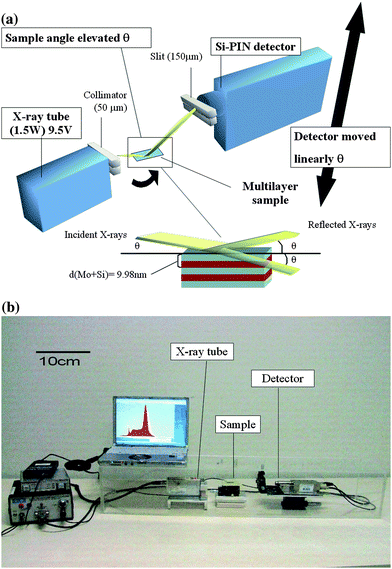 | ||
| Fig. 1 a) A schematic view of the portable X-ray reflectometer; fixed X-ray tube, sampled radially elevated θ and detector heightened at a position corresponding to 2θ; and b) A photograph of the portable X-ray reflectometer. | ||
Apparatus description
The design of the apparatus is not classical for an XRR instrument since it has an orthogonal geometry rather than a goniometric geometry, i.e. the X-ray tube, sample and detector are all in the same plane and the detector is moved linearly, not radially, unlike in a goniometer in the conventional apparatus. It is a portable apparatus, adaptable to a low-power X-ray source. In the apparatus we change the angle of the sample and the height of the detector according to the glancing angle at which the measurement is done. Although measurements for the different samples can be done at a fixed angle, changing the glancing angle and detector height is done to extra verify the results and make less error contribution to experiment. A low-power continuum X-ray source, adaptation to portability providing a portable set-up for X-ray reflectivity, straightforward and fast measurement and lower cost make this apparatus easier to use and more available to laboratories to substitute higher cost apparatus. Continuum X-rays and much lower power make it applicable without attenuation.The weight of the device, including the power supply amplifier, computer and other accessories, is less than 7 kg. The X-ray tube has a maximum voltage of 9.5 kV, a maximum current of 150 μA and a spot size of ∼50 μm (V) × 10 mm (H) (Manufacturer, Hamamatsu Photonics, model L9491 with W anode). The detector is an energy dispersive Si-PIN detector.14–19
Method description
In a Si-PIN detector; X-ray reflectivity of a multilayer is usually measured in a spectrometer as a function of glancing angle by illuminating the sample with a specific wavelength. A monochromatic X-ray beam irradiates a sample at a grazing angle θ while the reflected intensity is recorded at a height corresponding to 2θ. 2θ is the angle from the Bragg-diffracted in the reciprocal space to the Bragg-reflected beam in the real space in a lattice, where XRR reflection in multilayers resembles the Bragg condition in a lattice. In the present paper, X-ray reflectivity was measured as a function of energy at different angles. The X-ray tube; multilayer and detector are all on the same plane. The detector is aligned vertically. Since white radiation is used, the overall costs of energy-dispersive X-ray reflectivity measurement can be decreased by an order of magnitude. Measuring time was 600 s for each measurement. The applied voltage was 9.5 kV less than that for tungsten L3 absorption edge energy (10.2 keV) so tungsten L line characteristic X-rays were not emitted from the X-ray tube. A collimator (50 μm high; 10 mm wide; 12 mm long) was placed between the X-ray tube and the Mo/Si multilayer.A slit (150 μm) placed in front of the detector window, served to cut off the angular and spectroscopic tails of the continuum X-ray beam incident on the mirror. A Mo/Si multilayer sample (50 layers, d = 9.98 nm, dMo/d(Mo + Si) = 0.4) deposited by magnetron sputtering was measured.20 Elevating the sample, a white X-ray incident beam was fixed at a glancing angle θ. The reflected beam intensity was measured at an appropriate detector height corresponding to angle 2θ and reflectivity was calculated.
Results and discussion
X-ray reflectivity (XRR) for the Mo/Si multilayer was calculated, inputting the multilayer parameters, using Berkeley Laboratory X-ray tools.21 Reflectivity obtained by the portable X-ray apparatus was compared to calculated X-ray reflectivity. Reflectivity is obtained by dividing the intensity at a glancing angle by the intensity at 0.00°. Fig. 2 shows the data obtained by the apparatus at 0.00°, 0.45°, 0.60° and 0.80° as intensity versus X-ray energy. The spectrum at 0.00° shows the intensity of the direct beam, it decays at 0.45° and further decays at 0.60° and 0.80°. Fig. 3 shows the experimental and the theoretical results of X-ray reflectivity as a function of X-ray energy at 0.45°, 0.60° and 0.80°. The relative zero was taken at 0.02°. Measurement angle can slightly differ from theoretical angle by ±0.02°. The decay of the total reflection as the glancing angle is getting further from 0.00° is shown. The peak following is the first Bragg peak. Considering the geometry of the apparatus, a calibration equation for reflectivity was obtained. The intensity supposed to reach the detector is , where A(θ) is an empirical value. For unpolarised X-rays through a slit all values of intensity are detected with equal probability. The intensity is therefore averaged over cos2θ.
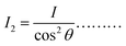 | (1) |
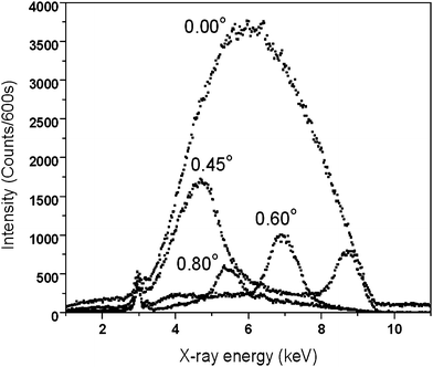 | ||
| Fig. 2 Intensity versus X-ray energy at (0.00°, 0.45°, 0.60°, 0.80°). Intensity at 0.00° is the direct beam. | ||
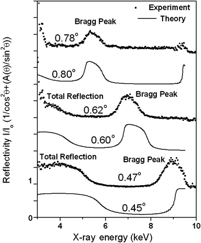 | ||
| Fig. 3 Reflectivity versus X-ray energy at (0.45°, 0.60°, 0.80°). The decay of the total reflection is followed by the first Bragg peak. | ||
cos2θ and sin2θ are expressed in terms of intensity as illustrated as follows:
 | (2) |
 | (3) |
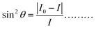
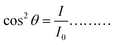
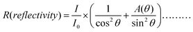
A(θ) is an empirical value supposedly dependent on the angular deviation, the experimental and theoretical curves are in good agreement when A(0.45°) = 0, A(0.60°) = 1.2 and A(0.80°) = 4. Fitting with the experimental results leads to a nonlinear response curve that can be fitted with good approximation with the following calibration equation:
 | (4) |
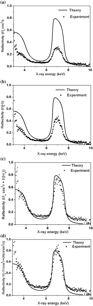 | ||
Fig. 4 Reflectivity versus energy by the calibration equation at 0.60°. (a) Measured Reflectivity of experimental X-ray intensity versus X-ray energy compared with the net calculated reflectivity versus X-ray energy at 0.60°; 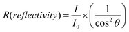 . (b) Measured Reflectivity of experimental X-ray intensity versus X-ray energy compared with the net calculated reflectivity versus X-ray energy at 0.60°; . (b) Measured Reflectivity of experimental X-ray intensity versus X-ray energy compared with the net calculated reflectivity versus X-ray energy at 0.60°; 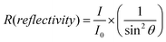 . (c) Measured Reflectivity of the sum of X-ray intensities versus X-ray energy compared with the net calculated reflectivity at 0.60°; . (c) Measured Reflectivity of the sum of X-ray intensities versus X-ray energy compared with the net calculated reflectivity at 0.60°; 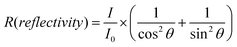 . (d) Measured Reflectivity of the sum of X-ray intensities, adding the radial constant, versus X-ray energy compared with the net calculated reflectivity at 0.60°; . (d) Measured Reflectivity of the sum of X-ray intensities, adding the radial constant, versus X-ray energy compared with the net calculated reflectivity at 0.60°; 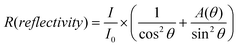 . . | ||
The sharp peak at around 3 keV in the experimental spectrum is due to the Ar Kα peak. The experimental curves are less corresponding to the theoretical curves as the region of X-ray total reflection gets sharper. This can be to some extent due to instrumental effects like imperfect collimation and the degree of inaccuracy. The Bragg peak in the theoretical and experimental spectra is more corresponding at 0.45° than at 0.60°, which in turn is more corresponding than at 0.80°.
From Fig. 3 thickness is directly obtained by the Bragg condition; e.g. the Bragg peak at 0.45° (0.007rad) corresponds to 8.70 keV (0.14 nm); applying the Bragg condition (2d sinθ = nλ), thickness will be 9.53 ± 0.45 nm. The intensity difference calibrated in the suggested problem does not contribute to this value since thickness is deducted from the Bragg peak position.
This slight difference and the difference in theoretical and experimental spectra in all the measurements were due to some problems concerning the accuracy of analysis. Any slight misalignment of the detector height could result in a less accurate detection angle of the reflected X-rays. As a result; reflectivity distribution might have changed and the X-ray flux might not be strong enough at 2θ. A shift of peaks with increasing angle might have been due to this reason. This might have resulted in lower reflectivities at 0.60° and 0.80°. The intensity was very weak in the range below 2 keV because of the Be window. The mode of operation was a θ/2θ mode (where θ is the glancing angle and 2θ is the detection angle) which assures the incident angle is always half of the angle of diffraction. The detector is heightened linearly with an instrument error of a micrometre. This can overall be a reasonable measurement since 1–10% variation of thickness and density happens after multilayer fabrication due to surface effects. Bulk density is always assumed in the calculated curves.
Although the detection angle is moved linearly, the X-ray portable reflectometer is adequate for detecting the reflecting beams due to small glancing angles and a calibration eqn (4) has been proposed. Since polarisation makes negligible contribution at small angles; unpolarised X-ray beam was used in the experiment. Because the reflection at the surface and interface is due to the different electron densities in the different layers, which correspond to different refractive indices, an error is always present in a sample. The average density near the surface in a multilayer is less than the normal bulk value and presumably increases with depth. Oxidation can also occur during and after multilayer preparation; that might contribute to the error.
Since the (Mo/Si) multilayer surface was glossy and white X-rays were used, specular reflection might not have been maintained and a combination of specular and diffuse reflection might have reflected off the multilayer surface.
Conclusion
Despites its simple principle, the apparatus fulfils industrial needs in portable thin layer thickness measurement. Reference samples are needed for calibration though reference samples of known thickness are not needed. Further reduction of size and weight by highly integrated and miniaturised electronics is planned.In the present paper we proved that continuum X-rays can be used for X-ray reflectivity measurement with a weak (1.5 watts) X-ray source. It provides the advantages of a continuum X-ray source in X-ray reflectivity; in terms of easiness of measurement; not associated with its usual problems related to strong intensity like sample damage, attenuation and provides less polychromatic effects. It also provides a portable apparatus for X-ray reflectivity. The portable apparatus presented is verified applicable in X-ray reflectivity measurement.
Acknowledgements
The present research was financially supported by the Japanese Ministry of Education, Science, Sport and Culture and SENTAN, JST. The authors are grateful to Dr Hisataka Takenaka (NTT-AT) for the supply of the Mo/Si multilayer sample used in the present research and useful discussion.References
- L. G. Parratt, Phys. Rev., 1954, 95, 359–69 CrossRef; B. L. Henke, Phys. Rev., 1972, A6, 94–104; D. K. G. de Boer, Phys. Rev., 1991, B4, 498–511.
- A. D. Dane, A. Veldhuis, D. K. G. de Boer, A. J. G. Leenaers and L. M. C. Buydens, Physica, 1998, B253, 254–68 Search PubMed; T. Salditt, D. Lott, T. H. Metzger, J. Peisl, G. Vignaud, J. F. Legrand, G. Gruebel, P. Hoghoi and O. Schaerpf, Physica, 1996, B221, 13–7 Search PubMed.
- B. K. Tanner and J. M. Hudson, IEEE Trans. Magn., 1992, 28, 2736–41 CrossRef CAS.
- J. Kawai, M. Takami, M. Fujinami, Y. Hashiguchi, S. Hayakawa and Y. Gohshi, Spectrochim. Acta, 1992, B47, 983–91; K. Hayashi, H. Amano, T. Yamamoto, J. Kawai, Y. Kitajima and H. Takenaka, Spectrochim. Acta, 1999, B54, 223–6; K. Hayashi, J. Kawai, Y. Moriyama, T. Horiuchi and K. Matsushige, Spectrochim. Acta, 1999, B54, 227–30.
- K. Hayashi, S. Kawato, T. Horiuchi, K. Matsushige, Y. Kitajima and J. Kawai, Appl. Phys. Lett., 1996, 68, 1921–3 CrossRef CAS.
- J. Kawai, M. Sai, T. Sugimura, K. Hayashi, H. Takenaka and Y. Kitajima, X-Ray Spectrom., 1999, 28, 519–22 CAS.
- P. Karimov, S. Harada and J. Kawai, Surf. Interface Anal., 2003, 35, 76–9 CrossRef CAS.
- V. R. Albertini, B. Paci and A. Generosi, J. Phys., 2006, D39, R461–R86.
- S. Kunimura and J. Kawai, Anal. Chem., 2007, 79, 2593–5 CrossRef CAS.
- A. Carapelle, K. Fleury-Frenette, J. Collette, H. Garnir and P. Harlet, Rev. Sci. Instrum., 2007, 78, 123109–1 CrossRef; A. Attaelmanan, S. Larsson, A. Rindby, P. Voglis and A. Kuczumow, Rev. Sci. Instrum., 1994, 65, 7–12 CrossRef CAS; C. Ribbing, M. Anderson, K. Hjort and H. Lundqvist, Rev. Sci. Instrum., 2003, 74, 3423–8 CrossRef CAS.
- A. Longoni, Nucl. Instrum. Methods, 1998, 409A, 407–9 Search PubMed.
- P. Dhez, H. Duval and J. C. Malaurent, J. X-ray Sci. Technol., 1992, 3, 176 CrossRef.
- L. Kaihola, E. L. J. C. Malaurent, H. Duval and P. Dhez, J. Magn. Magn. Mater., 1991, 93, 176–93.
- B. Lengeler, Adv. Mater., 1990, 2, 123 CAS.
- J. C. Malaurent, H. Duval, J. P. Chauvineau, O. Hainaut, A. Raynal and P. Dhez, Opt. Commun., 2000, 173, 255–63 CrossRef CAS.
- T. C. Huang, R. Gilles and G. Will, Thin Solid Films, 1993, 230, 99–101 CrossRef CAS.
- R. Felici, Rigaku J., 1995, 12, 11–7 Search PubMed.
- K. Orita, T. Morimura, T. Horiuchi and K. Matsushige, Synth. Met., 1997, 91, 155–58 CrossRef CAS.
- P. Karimov, S. Harada, H. Takenaka and J. Kawai, Spectrochim. Acta, 2007, B62, 476–80.
- H. Takenaka, T. Kawamura and H. Kinoshita, Thin Solid Films, 1996, 288, 99–102 CrossRef.
- Berkeley Lab. (http://henke.lbl.gov/optical_constants/multi2.html).
| This journal is © The Royal Society of Chemistry 2010 |