High-throughput surface plasmon resonance imaging-based biomolecular kinetic screening analysis†
Ganeshram
Krishnamoorthy
*,
J.
Bianca Beusink
and
Richard B. M.
Schasfoort
BIOS Lab-on-a-Chip Group, MESA+ Institute for Nanotechnology, University of Twente, P.O. Box 217, 7500 AE, Enschede, the Netherlands. E-mail: g.krishnamoorthy@utwente.nl; Fax: +31-53-4893595; Tel: +31-53-4892724
First published on 28th May 2010
Abstract
In this paper we show a high-throughput method to screen the kinetics and affinity constants of many biomolecular interactions simultaneously. During the preparation of the sensor chip, ligands were serially diluted and spotted in a 6 × 4 microarray on the sensor surface. A multi-analyte sample was injected and the real-time surface plasmon resonance (SPR) responses of all the 24 microarray spots were obtained using a commercial SPR imaging instrument. The multi responses of the association and dissociation processes obtained from a single analyte injection are sufficient to calculate the rates and affinity constants of the interactions between three interactant antigen-antibody pairs using a simple monophasic kinetic model. The method drastically reduces the measurement time and cost in the benefit of increased throughput.
Introduction
Biomolecular interactions can be analyzed using direct label-free biosensing techniques1–3 and the information can be used in various ways, such as, to quantitate binding specificity, and rate and affinity constants4 of two or more interactants. Surface plasmon resonance based biosensor technology is widely accepted as the standard label-free detection technique to measure real-time biomolecular interactions. However, the number of biomolecular interactions that can be monitored in conventional direct biosensor systems is typically limited. In conventional procedures, ligands are immobilized on the sensor surface and analytes of various concentrations are injected in several runs to evaluate kinetics using overlay plots for calculating the association rate, dissociation rate and affinity constants. The evaluation of kinetics using multiple ligands is therefore very time-consuming. The advancement in SPR imaging leads to high-throughput approaches. Currently, there are many commercially available iSPR systems, including the Biacore Flexchip,5 GWC SPRimagerII,6 IBIS-iSPR,7–9 Genoptics SPRi-Lab+,10 and also many custom-made iSPR systems.11,12An advantage of the approach presented here is to apply the enormous capacity of a microarray by immobilizing several ligands in serial dilution and using SPR imaging to perform kinetic experiments (up to 500 spots) with analytes that bind specifically to the ligands. With the inclusion of regeneration steps, the analytes can also be injected serially. However, if the kinetics are to be evaluated using a single analyte concentration and serial dilution of spotted ligands, then in principle a regeneration step is not necessary. Although kinetics have been evaluated through various ligand concentrations in a four channel instrument with single analyte concentration13,14 the implication is that SPR imaging will contribute to the analysis of, in principle, hundreds of different ligand to analyte bindings; many interactions can be performed simultaneously including reference and duplicate spots. We have recently showed the concept of extracting kinetics with just single injection of analytes over the microarray where multiple concentrations of ligands are immobilized.9 In this paper, we show the extended approach (as described in Ref. 9, fig. 1f) of estimating kinetics and affinity constants of multiple (three) interactant pairs with single injection of mixture of analytes as a proof of concept.
Theoretical aspects
The kinetic model for a 1![[thin space (1/6-em)]](https://www.rsc.org/images/entities/char_2009.gif) :1 interaction is normally represented by eqn (1) and (2):
:1 interaction is normally represented by eqn (1) and (2):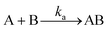 | (1) |
 | (2) |
 | (3) |
The ligands are immobilized on the sensing surface by spotting in serial dilution in a micro array format. The immobilized ligands have different densities as well as different orientations on the sensor surface. The interactions are measured at several regions of interests on various spots simultaneously in real time. The observed signal, Rt, is proportional to the formation of AB complexes at the surface with respect to the ligand density. Accordingly, the maximum signal, Rmax (maximum capacity of ligands that bind with analytes without any dissociation of the complex AB), will then be proportional to the surface density of active ligand at the surface. If one uses different ligand types, then Rmax varies with respect to the ligand spots of the microarray. In this case, for a single spot, the complex formation rate is,
 | (4) |
 | (5) |
The time dependent response Rt is therefore,
 | (6) |
This is the general equation for a monophasic biomolecular interaction with stoichiometry 1:1.15
Note that if we apply a single analyte injection to different spots, the analyte concentration has a constant value (does not change with respect to various ligand densities) and Rmax varies at different spots and directly depends on the ligand density which is also an indirect estimation of ligand concentrations on the surface. The assumption being the analyte concentration used is far too higher the immobilized ligand density which is similar to that of the conventional 1:1 interaction model.13 Additionally, if ligands are serially diluted at different spots on the sensor array, then Rmax is dependent on the spot ligand density. The Rmax value can be obtained from the ligand response before the injection step for all the spots by subtracting it with that of a blank measurement. Rmax depends on the stoichiometry of the interaction and the ratio of molecular weight of the ligand the molecular weight of the analyte.
 | (7) |
 | (8) |
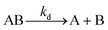
In eqn (8), there is a need for extra parameter (for e.g. “x”) to represent the number of active sites on the ligand that could interact with the analytes. More detailed analysis of such constants has to be evaluated experimentally and it is still under investigation in our lab. To demonstrate the method of kinetics evaluation, we proceed with the assumption that the model systems just follows 1:1 interaction model. The dissociation rate can be found during the dissociation phase and is only dependent on the concentration of the formed complex ‘AB’ which is proportional to Rt and given by
 | (9) |
In this paper, we want to show that the rate ka and kd constants and affinity constant KD can be obtained from the derivative of eqn (6) to the variable Rmax in different spots. In a plot of Rtversus Rmax, the slope (dRt/dRmax) can be determined, where
 | (10) |
All parameters in eqn (10) are known except ka. At a certain time t after injection and using a certain analyte concentration [A], the association rate constant ka can be numerically determined from eqn (10). Therefore, single injection multi kinetics can be performed using different ligands each serially diluted on the surface and applying moderate analyte concentration. In this paper this model has been applied to our microarray results and the relevance of this approach is discussed.
Materials and methods
Microarray fabrication
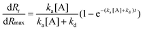
A pre-activated functionalized hydrogel sensor chip (HCX 80m, XanTec, Germany) was used in this experiment. A non contact printing system “TopSpot” (BioFluidix, Germany),16 was used to spot different ligands on the sensor surface. The 24-spot microarray consisted of four different concentrations (100, 200, 400 and 800 μg ml−1) of human IgG, bovine IgG and BSA with duplicates, as shown in Fig. 1. The sensor was incubated for 1 h in a humidity chamber at room temperature for immobilization process. After immobilization, the remaining active groups of the sensor surface were quenched with ethanolamine (1 M, pH 8) for 10 min in order to prevent non-specific binding of interfering proteins.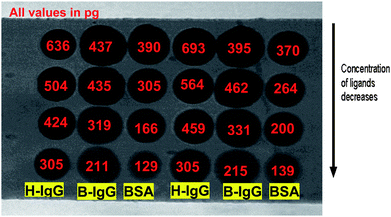 | ||
| Fig. 1 iSPR image of the microarray fabricated using TopSpot for the three interactant pairs. Columns 1 and 4 – Human IgG, Columns 2 and 5 – Bovine IgG and Columns 3 and 6 – BSA; The concentration of the ligands in the immobilization buffer decreases (800, 400, 200 and 100 μg ml−1) from row 1 to row 4 which is indicated by the arrow. The true ligand surface density, which is assumed to be proportional to Rmax, was calculated from the response Rt with respect to background after washing the microarray intensively (according to calibration experiments, 1 millidegree angle shift is equal to 10.8 pg mm−2 of protein on the surface). All the values mentioned in the figure are ligand densities in picograms/ROI in a spot of 150 × 150 microns. The gradual decrease of the ligand density is close to the saturation level and is not linear with the applied ligand concentration. | ||
Detection of biomolecular interactions on the protein microarray
The sensor containing the protein microarray was mounted in the IBIS-iSPR from IBIS Technologies BV, The Netherlands. The principle of the new scanning angle IBIS-iSPR has recently been explained in the literature.7–9 A collimated beam of light is shined to the hemispherical prism where the gold sensor disk is coupled (using the same refractive index oil). At certain critical angle, all the light hitting the prism is completely reflected back termed as “total internal reflection”. During this process, the photons of light coupled to the surface plasmons on the metal surface that forms surface plasmon polaritons which propogates on the surface and travels in the form of waves on the metal surface. The reflectivity go to the minimum during this process (SPR dips) and is plotted with respect to time domain called sensorgram which contains the SPR angle shift (millidegrees, m°) on the ordinate and measurement time on the abcissca. A refractive index change at the solution/gold interface is related to the amount of adsorption or binding of biomolecules at the surface, which results in a measurable shift of the SPR-dip. The SPR angle shift is used as a response unit (RU) to quantify the binding of biomolecules to the sensing surface. There are three main measurement phases of the sensorgram; 1) baseline phase: a running buffer in contact with the sensor surface to establish the baseline responses, 2) association phase: sample containing the target analyte [A] is injected to the interaction chamber and the ligands [B] immobilized on the surface, the capturing element on the sensor surface binds to the target resulting in complex formation [AB], and 3) dissociation phase: injection of a running buffer again which leads to dissociation of bound molecules from the surface. The system was equilibrated using 1 mL PBS-Tween in the flow-cell at a flow-speed of 2 μL s−1 at 25 °C. After defining the ROIs of 20 × 20 pixels each, corresponding to 150 × 150 μm, the SPR-dip was measured automatically by the IBIS-iSPR software (see ESI†).Three analytes 27 nM anti-human IgG (Zymed, USA), 32 nM anti-bovine IgG (Jackson Immunoresearch, USA) and 60 nM anti-BSA (Sigma, the Netherlands) were mixed and the analyte mixtures were injected to the sensor surface. The association phase responses were measured for 1000 s followed by a 2000 s dissociation phase measurement, which was prolonged due to a slow dissociation process. Data analysis was performed with ISPRAD software (IBIS, the Netherlands) and classical kinetics analysis was performed using Scrubber 2 (Biologic, Australia).17 Microsoft Excel was used for the kinetics evaluation in this paper and was compared to the classical approach using regeneration steps and serial diluted analyte concentrations and overlay plots as described elsewhere.18
Results and discussion
The advantage of our microarray-based kinetics evaluation is that one can easily measure the kinetics of multiple systems with a single injection step, if the ligand spots are immobilized in different densities on the microarray. In principle, the association and dissociation times can be reduced further which should not influence the kinetic rate and affinity results in the non-equilibrium situation. If the ligand has a certain molecular weight and the different ligand densities can be determined prior to analyte injection which leads to the estimation of Rmax. The analyte response, with correction for the bulk refractive index shift, was determined as the angle-shift after the association phase just after injection of the dissociation buffer. The sensor can be regenerated with glycine-HCl (pH 2.0) after each analysis cycle. However a regeneration step is in principle not necessary for our new multikinetics approach since a single injection of the analytes results in various binding curves.In Fig. 1, the column 1 and 4 has spots of human IgG and the concentration decreases from top to bottom. The second & fourth and third & sixth column contains spots of bovine IgG and BSA respectively. The area occupied by the 1 nL sample for various protein molecules is different and clearly represents the different wettabilities of the sensor surface due to these surface immobilized proteins.19 In our case, bovine IgG protein spots show a larger surface area with respect to BSA and human IgG, which indicates a more hydrophilic nature of the bovine IgG protein. Regeneration of these hydrophilic spots was more difficult than the others and the classical approach using several analyte concentrations, regeneration steps and overlay plots was not easy for the bovine IgG protein spots (results not shown in this paper).
All the three model interactant pairs used in this work is multi-valent in nature. So the stoichiometry is not 1 in these cases. But when the concentration used is very less, it does follow 1:1 interaction model without any fit problem. For demonstration of the concept and simplicity purpose, we use these well defined interactant pairs with the most simplified model described in this paper. The new procedure to calculate the rate and affinity constants from the obtained SPR imaging data are shown here. Since we used non contact printing for ligand immobilization on the microarray, the density of immobilized ligand on the surface can be estimated from the initial measured response just after spotting as indicated in Fig. 1. Although we are not aware of the effective ligand density (part of protein can be denatured, blocked or inactive), we assume that there is a direct relation between measured response after immobilization and Rmax which is a ratio of the molecular weights of the analytes to the ligands. Therefore, Rmax can be calculated for each spot if we assume a 1:1 biomolecular interaction stoichiometry. We found that Rmax is not proportional to the ligand concentration CL, which means that droplet depletion, droplet drying effects including changed immobilization efficiencies and kinetics should be taken into account during the spotting process. The ligand concentration CL of each droplet in the printing system is different than the effective density of the immobilized ligand. The exact ligand density is estimated from the SPR dip shift of the spot with respect to the background of the microarray (non coated surface which in other words is called blank control spot). A baseline corrected sensorgram for all 8 BSA spots is shown in Fig. 2.
 | ||
| Fig. 2 Sensorgram (response versus time) obtained for the BSA–antiBSA interactant pair with varying ligand density is shown here. The noise in the curves is a result of the hydrodynamic back and forth pumping of the sample in the flow cell, but is not affecting the kinetics. The total association time is 1000 s and total dissociation time is 2000 s. The “green” colour plot indicates a spot exposed to 100 μg ml−1 ligand and with ∼129 pg/ROI, the “red” colour plot indicates 200 μg ml−1 with relatively large deviation in the duplicate spot (∼166 pg/ROI), the “blue” colour indicates 400 μg ml−1 (∼305 pg/ROI) and the “black” colour indicates 800 μg ml−1 (∼390 pg/ROI) of BSA that was used for immobilizing ligand on the surface respectively with duplicates. | ||
The method used to calculate the total amount of immobilized proteins on the spot is explained here by considering the sensorgram of 60 nM antiBSA injections on a spot exposed to 800 μg ml−1 BSA. As seen in the Fig.2, Rmax ≈ 248 m°. As we know from calibration experiments for the IBIS iSPR systems,8 we use an empirical result that 1 m° response (angle shift) is equal to 10.8 pg mm−2 of protein on the surface. From the area of the ROI used for measuring the response, the amount of BSA on the surface for this spot is 390 pg. This shows that the actual concentration of ligand in buffer can be very different from the immobilized ligand densities. The exact amount of immobilized ligand is necessary for the kinetics evaluation in order to show the calculation of the actual ligand density. The real protein densities were measured for all the spots and are shown directly on the spots in Fig. 1. Because the analyte is a mixture of three antibodies, the immobilized ligand has many epitopes which may bind the antibody, a one-one interaction (S = 1) of the analyte to the ligand is therefore a very rough assumption. As indicated in the Table 1 it was clearly revealed that the real process of binding does not show 1:1 stoichiometry because the response (Rt) for the anti-BSA interaction is higher than Rmax. For the other model interactant pairs, direct co-relation was clearly observed between ligand density and the Rmax values.
| Interactant pairs | R max | Response | Slope | Results |
|---|---|---|---|---|
| Human IgG | 392 | 93 | 0.31 | K D = 295 pM |
| 311 | 92 | k a = 1.7 × 10⁵ M−1 s−1 | ||
| 262 | 82 | k d = 5.1 × 10⁻⁵ s−1 | ||
| 188 | 57 | |||
| Bovine IgG | 270 | 88 | 0.49 | K D = 58 pM |
| 268 | 83 | k a = 1.6 × 10⁵ M−1 s−1 | ||
| 197 | 80 | k d = 9.4 × 10⁻⁶ s−1 | ||
| 130 | 65 | |||
| BSA | 241 | 228 | 0.98 | K D = 895 pM |
| 188 | 211 | k a = 5.8 × 10⁴ M−1 s−1 | ||
| 103 | 159 | k d = 5.2 × 10⁻⁵ s−1 | ||
| 79 | 126 |
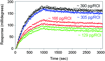
A sensorgram with raw data, including noise from the back and forth hydrodynamic pumping, was used directly for the calculations. It will not influence the final kinetics and affinity results because the slope dRt/dRmax is not going to change because of noise and bulk shift responses. All spots are exposed to the same analyte concentration and bulk refractive index. The plot was made with Rmax on the “X” axis and Rt on the “Y” axis. The data were fitted linearly and the slope was determined.
Deviations from linearity indicates that the interaction does not follow a simple monophasic model anymore and there may be influences from steric hindrances, mass transport limitations,20 re-binding effects and/or other effects. Since we use a mixture of monoclonal antibody as an analyte, we understand that in principle the 1:1 monophasic binding model is an oversimplification of the overall interaction. However this paper shows a comparison of calculating the rate and affinity constant using the classical approach with overlay plots with respect to calculating the constants with the single multikinetic approach with slope (dRt/dRmax) using eqn (10). The dissociation rate, kd can be calculated classically from the dissociation phase using kd = −(dRt/dt)/Rt. Knowing the value of [A], which is constant throughout the experiment, the association rate, ka can be calculated from eqn (10) because we already calculated the slope from the plot of Rtversus Rmax, shown in Fig. 3. With known kd and ka the affinity constant KD is calculated using eqn (3). The association rate, dissociation rate and affinity constant of human IgG–antihuman IgG interactions is 1.7 × 10⁵ M−1 s−1, 5.1 × 10⁻⁵ s−1 and 295 pM, respectively. The association rate, dissociation rate and affinity constant of bovine IgG–antibovine IgG interactions are 1.6 × 10⁵ M−1 s−1, 9.4 × 10⁻⁶ s−1 and 58 pM respectively. The association rate, dissociation rate and affinity constant of BSA–antiBSA interactions is 5.8 × 10⁴ M−1 s−1, 5.2 × 10⁻⁵ s−1 and 895 pM respectively. The values of Rmax, responses, slopes, association rates, dissociation rates and affinity constants are shown in Table 1 for all the three interactant pairs used in our experiment.
 | ||
| Fig. 3 Single injection multi-kinetics evaluation of all the 3-interactant pairs. RtversusRmax (see discussion) and is plotted for the ligand–analyte combinations. The rate and affinity constants are calculated from the initial slope (dRt/dRmax). However the determination of the slope of bovine IgG is not accurate and based on a single RtversusRmax value. Generally at higher Rmax values, the plot will deviate from a simple monophasic model which indicates that e.g. mass transport limitation, changed stoichiometries, rebinding effects or steric hindrances should be taken into account. | ||
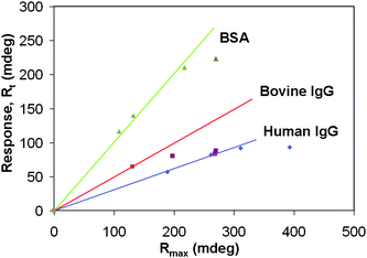
Additionally, the deviation from the linear fit of the slopes for the higher ligand density spots of the interactant pairs is a clear indication that these interactions do not follow a simple monophasic model as was also indicated by the classical kinetics evaluation software “Scrubber”. These data points fit better to models with mass transport limitations included. The calculation of the rates and affinity constant for the BSA–antiBSA interaction using the traditional method with varying analyte concentrations and overlay plot using Scrubber is shown in Fig. 4. Knowing the fact that the anti-BSA is the partitioning solute and is much larger than the immobilized albumin molecule, in which case the kinetic analysis is complicated by the parking problem that arises when a partitioning solute molecule can cover more affinity sites than the one to which it is actually complexed.21 But we don't see any deviation of experimental results to the model fit in our case.
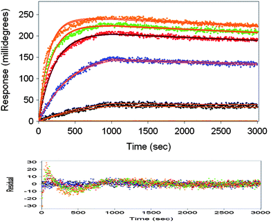 | ||
| Fig. 4 Classical kinetics and affinity evaluation for BSA–antiBSA interactions by varying analyte concentrations and over lay plots. The residual plot for the obtained fit is shown in plot at the bottom. The calculated affinity constant is 880 pM. | ||
The extracted kinetics of all three interactant pairs with varying ligand densities and single analyte concentrations does not show a large deviation from the traditional approach. The comparisons of the relevant results are shown in Table 2.
| Interactant pairs | Traditional kinetics (pM) | Single injection kinetics (pM) | Single injection multikinetics (pM) |
|---|---|---|---|
| Human IgG–antihuman IgG | 203 | 278 | 295 |
| Bovine IgG–antibovine IgG | 59 | 78 | 58 |
| BSA–antiBSA | 880 | 1060 | 895 |
A single injection multikinetics approach reduces the time of kinetic experiments drastically as well as the cost for the measurement as we just need a single sensor chip and only one injection of an (sometimes expensive) analyte. The method described in this paper is comparable to that of an approach described elsewhere,22 however using SPR microarray imaging the number of simultaneous biomolecular interactions can be improved significantly and up to 500 spots with the SPR imaging system we applied for this experiment. As long as the ligand density is small and analyte concentration is near the real affinity value of the interactant pairs, as well as no cross reaction (non-specific binding) is observed, this new approach can be implemented to biomolecular interaction data in a straight forward manner. Considerations to mass transport limitations, rebinding effects, steric hindrance in hydrogels and other factors that may complicate the simple 1:1 binding model should be taken into account and low ligand densities are always the best to determine kinetic rate constants. We recommend for future analysis a biomolecular interaction set that fits exactly a monophasic binding model or use a model that can be applied for the interaction couple of interest. More advanced models, for example, distribution analysis models23,24 may be a solution for these problems. Also, the approach could be optimized by integrating Lab-on-a-Chip based microfabricated devices to the SPR imaging biosensing systems as reported in the literature.25 However, microfabrication makes the device more expensive sometimes and it depends on the how complicated procedures are handled for the fabrication of biochips.
Conclusion
The procedure to apply single injection multi-kinetics for fast analysis of affinity constants using surface plasmon resonance imaging is demonstrated in this paper. The rate and affinity constants were calculated for three interactant pairs with a single injection of mixture of analytes. Although the calculation of the absolute affinity constants with the simple monophasic model and assumed 1:1 stoichiometry for antigen and polyclonal antisera is questionable, comparison of the traditional method with the single injection multikinetics approach is performed in this study. The results obtained from the single injection multi-kinetics for all the three interactant pairs corresponds well to those obtained from the traditional approach. However the single injection multikinetics approach leads to a dramatic reduction of measurement time from hours to a single injection. Data handling of kinetic results from several analyte concentrations into overlay plots are not necessary. For each ligand, 4 to 5 dilutions should be sufficient to get a good indication of the affinity constants. However for accurate estimations, the ligand densities should be as low as possible with sufficient Rmax above the signal to noise ratio of the instrument. From the slopes (dRt/dRmax) of the plot Rtversus Rmax, the association rate constants of the different analyte-ligand combinations can be determined independently if a high selectivity of the antigen/antibody interaction and no significant cross-reactivity occurs. The affinity value (KD) obtained from the single injection multikinetics method with the consideration that the monophasic model is an oversimplification of the real binding process is for human IgG–antihuman IgG 295 pM, bovine IgG–antibovine IgG 58 pM, and for BSA–antiBSA 895 pM respectively.Acknowledgements
The authors thank the Dutch organization for scientific technological research “STW” for funding the project TMM 6635. The authors thank Prof. Albert van den Berg and Dr Edwin Carlen of the BIOS, Lab on a Chip group of MESA+ Institute for Nanotechnology for their valuable suggestions.References
- P. R. Edwards, A. Gill, D. V. Pollard-Knight, M. Hoare, P. E. Buckle, P. A. Lowe and R. J. Leatherbarrow, Anal. Biochem., 1995, 231, 210–217 CrossRef CAS.
- P. R. Edwards and R. J. Leatherbarrow, Anal. Biochem., 1997, 246, 1–6 CrossRef CAS.
- P. Schuck, Annu. Rev. Biophys. Biomol. Struct., 1997, 26, 541–566 CrossRef CAS.
- R. Karlson, A. Michaelsson and L. Mattsson, J. Immunol. Methods, 1991, 145, 229–240 CrossRef CAS.
- D. G. Myszka and R. L. Rich, PSTT, 2000, 3, 310–317 Search PubMed.
- B. P. Nelson, T. E. Grimsrud, M. R. Liles, R. M. Goodman and R. M. Corn, Anal. Chem., 2001, 73, 1–7 CrossRef CAS.
- A. M. C. Lokate, J. B. Beusink, G. A. J. Besselink, G. J. M. Pruijn and R. B. M. Schasfoort, J. Am. Chem. Soc., 2007, 129, 14013–14018 CrossRef CAS.
- J. B. Beusink, A. M. C. Lokate, G. A. J. Besselink, G. J. M. Pruijn, R. B. M. Schasfoort and Biosens, Biosens. Bioelectron., 2008, 23, 839–844 CrossRef CAS.
- G. Krishnamoorthy, E. T. Carlen, J. B. Beusink, R. B. M. Schasfoort and A. van den Berg, Anal. Methods, 2009, 1, 162–169 RSC.
- B. Cherif, A. Roget, C. L. Villiers, R. Calemczuk, V. Leroy, P. N. Marche, T. Livache and M. B. Villiers, Clin. Chem., 2005, 52, 255–262 CrossRef.
- N. Bassil, E. Maillart, M. Canva, Y. Levy, M. C. Millot, S. Pissard, R. Narwa and M. Goossens, Sens. Actuators, B, 2003, 94, 313–323 CrossRef.
- I. Mannelli, V. Courtois, P. Lecaruyer, G. Roger, M. C. Millot, M. Goossens and M. Canva, Sens. Actuators, B, 2006, 119, 583–591 CrossRef.
- P. R. Edwards, P. A. Lowe and R. J. Leatherbarrow, J. Mol. Recognit., 1997, 10, 128–134 CrossRef CAS.
- I. Chaiken, S. Rose and R. Karlsson, Anal. Biochem., 1992, 201, 197–210 CAS.
- D. J. O'Shannessy and D. J. Winzor, Anal. Biochem., 1996, 236, 275–283 CrossRef CAS.
- B. de Heij, M. Daub, O. Gutmann, R. Niekrawietz, H. Sandmaier and R. Zengerle, Anal. Bioanal. Chem., 2004, 378, 119–122 CrossRef CAS.
- T. A. Morton, D. G. Myszka and I. M. Chaiken, Anal. Biochem., 1995, 227, 176–185 CrossRef CAS.
- R. L. Rich and D. G. Myszka, J. Mol. Recognit., 2006, 19, 478–534 CrossRef.
- A. A. Kortt, E. Nice and L. C. Gruen, Anal. Biochem., 1999, 273, 133–141 CrossRef CAS.
- P. Schuck and A. P. Minton, Anal. Biochem., 1996, 240, 262–272 CrossRef CAS.
- D. Hall and D. J. Winzor, Int. J. Biochromatogr, 1999, 4, 175–186 Search PubMed.
- T. Bravman, V. Bronner, K. Lavie, A. Notcovich, G. A. Papalia and D. G. Myszka, Anal. Biochem., 2006, 358, 281–288 CrossRef CAS.
- J. Svitel, A. Balbo, R. A. Mariuzza, N. R. Gonzales and P. Schuck, Biophys. J., 2003, 84, 4062–4077 CrossRef CAS.
- J. Svitel, H. Boukari, D. Van Ryk, R. C. Willson and P. Schuck, Biophys. J., 2007, 92, 1742–1758 CrossRef CAS.
- E. Ouellet, C. Lausted, T. Lin, C. W. T. Yang, L. Hood and E. T. Lagally, Lab Chip, 2010, 10, 581–588 RSC.
Footnote |
| † Electronic supplementary information (ESI) available: SPR dip obtained directly from the iSPR instrument which represents the variation of duplex spots that were spotted on the surface (BSA spots). See DOI: 10.1039/c0ay00112k |
| This journal is © The Royal Society of Chemistry 2010 |