Weighted partial least squares regression by variable grouping strategy for multivariate calibration of near infrared spectra

Abstract

A weighted partial least squares (PLS) regression method for multivariate calibration of near infrared (NIR) spectra is proposed. In the method, the spectra are split into groups of variables according to the statistic values of variables, i.e., the stability, which has been used to evaluate the importance of variables in a calibration model. Because the stability reflects the relative importance of the variables for modeling, these groups present different spectral information for construction of PLS models. Therefore, if a weight which is proportional to the stability is assigned to each sub-model built with different group variables, a combined model can be built by a weighted combination of the sub-models. This method is different from the commonly used variable selection strategies, making full use of the variables according to their importance, instead of only the important ones. To validate the performance of the proposed method, it was applied to two different NIR spectral data sets. Results show that the proposed method can effectively utilize all variables in the spectra and enhance the prediction ability of the PLS model.

---

Introduction

As a simple, rapid and non-destructive analytical technique, near-infrared (NIR) spectroscopy has been widely used in the analysis of complex samples, e.g., foods, agricultural products, Chinese traditional medicines and even bio-samples.^1–4 It is also seen as a promising tool for process analytical technology (PAT) in pharmaceutical production.⁵ For example, in the process analysis of an industrial production, it is hard to conduct an on-line analysis by using the conventional methods based on wet analysis. NIR spectroscopy, however, provides a powerful tool for process control. Nevertheless, most NIR spectra typically consist of broad, weak, non-specific and overlapping bands. Therefore, chemometric techniques are generally used to construct calibration models for the quantitative analysis of NIR spectroscopy. Among the chemometric techniques, partial least squares (PLS) regression is the most commonly used calibration method.^6–8 Furthermore, to obtain a satisfactory result for complex sample analysis, pretreatment techniques have been proposed to remove the background and noise in the spectra, e.g., multiplicative scattering correction (MSC),^9,10 the standard normal variate (SNV),^11,12 orthogonal signal correction (OSC),¹³ and wavelet transform (WT).^14–18

Another technique for improving the PLS modeling is to deal with the redundant variable. Generally, NIR data sets may have thousands of wavelengths, sometimes from hundreds or thousands of samples. Not all wavelengths in a spectrum, however, contain equivalent information relevant to the component of interest. Variable selection is a common way to gather wavelengths that do contain relevant information. Many variable selection methods have been developed, such as genetic algorithms (GA),^19,20 uninformative variable elimination by PLS (UVE-PLS),^21–25 interval PLS (iPLS),^26,27 variable selection based on randomization test for PLS (RT-PLS),²⁸ and variable selection based on truncation of weight vectors in PLS.²⁹ In our previous works, an integration of the Monte Carlo (MC) technique and UVE was proposed and named as MC-UVE.²⁵ These methods can significantly improve the performance of the calibration techniques by removing the irrelevant variables. On the other hand, some approaches have been proposed to extract the useful information from all variables regardless the relevancy.^30,31 Because, in the spectra of complex samples, some useful information may be embedded in the background and noise components, it is therefore difficult to determine the relevancy of a variable.^31,32 These approaches try to improve the quality of the calibration model by weighting all the variables instead of discarding some of them as done in wavelength selection methods.

In this study, a combined PLS model with variable grouping based on stability for multivariate calibration of NIR spectra is proposed. In the proposed method, all variables (wavelengths) are grouped by their stability and sub-models are built with the grouped variables. The same way as in MC-UVE²⁵ is adopted to calculate the stability for each variable. The objective is to construct a model with good prediction performance by keeping all wavelengths and making the best use of the information from all variables. In order to demonstrate the performance of the method, two NIR spectral data sets are investigated. The results indicate that the proposed method is a feasible way to enhance the prediction quality of the PLS model.

Theory and algorithm

Monte Carlo combined with uninformative variable elimination (MC-UVE)

MC-UVE is a method that combines Monte Carlo and uninformative variable elimination (UVE). It has been used for variable selection in NIR spectral modeling.^23,25 The method builds a large number of models with randomly selected calibration spectra by Monte Carlo technique at first, then stability of each variable is calculated by using the coefficients of these models, and each variable is evaluated with the stability. Variables with poor stability are known as uninformative ones and eliminated. The final PLS model for prediction of unknown samples is built by using the retained variables.²⁵

Weighted PLS with variable grouping (VG-PLS)

Stability is used in UVE method as a measurement of the reliability of variables for calibration. For UVE method, variables with high stabilities are used and other ones are deleted. In this work, stability is used to decompose the spectra into different groups, in this way these groups present different spectral information for construction of PLS models. Thus, it may be a good idea to build a PLS model by using all the variables with a suitable weighting strategy.

In order to use full spectral information in a calibration model, a method of weighted PLS with variable grouping for NIR spectra analysis is proposed in this study and named as variable grouping (VG)-PLS. VG-PLS model is a combination of the sub-models of the grouped variables. If w is used to denote the weight of a sub-model, the linear combination of the sub-models can be represented as:

ŷ = [ŷ₁,ŷ₂,ŷ₃…ŷ_n]w (1)

where n is the number of sub-models, and ŷ_i is a vector representing the prediction of the ith sub-model. The weight vector w is determined by the importance of each sub-model to the final prediction. Considering that the stability of each variable shows its reliability for modeling, the weight of the ith sub-models is defined as: where i and j represent the index of groups and the index of variables in each group, respectively, and c_j is the stability of each variable. m is a factor to adjust the contribution of each variable to the weight and to balance the weights of different groups.

The detail procedures of the VG-PLS can be described as follows:

(1) By using Monte Carlo technique like in MC-UVE,²⁵ the stability of the variables are calculated and will be used for grouping variables and deciding the weights of groups in the following steps.

(2) The variables in the spectra are ranked in a descending order of their stability.

(3) The variables are split into n groups. Each group contains almost the same number of variables following the order, and sub-models are built with the groups.

(4) The contribution of the sub-models to the combined model, i.e., the weights, is calculated by (2).

(5) The predictions of the prediction set are performed using the combined model, i.e., the variables of the validation spectra are split into n groups in the same order of step (3), then the n prediction values are produced by the n models, and finally a prediction is made by the weighted sum of the n values as shown in (1).

Clearly, m and n are two important parameters of the combined model, which will be discussed in the following sections. A validation set was used for optimization of the two parameters.

Experimental and calculations

Two NIR spectral data sets were used in this study. Data set 1 was downloaded from http://software.eigenvector.com/Data/Corn/index.html, which consists of NIR spectra, measured with three spectrometers, and the moisture, oil, protein and starch values of 80 corn samples. The spectra were measured on mp5 NIR spectrometer and the starch values are used in this study. Each spectrum was recorded in the wavelength range 2498–1100 nm (4003–9091 cm⁻¹) with the digitization interval 2 nm. Each spectrum is composed of 700 data points.

Data set 2 is supplied by a tobacco corporation, including the NIR spectra of 2199 tobacco lamina samples and the contents of sugar and nicotine. The spectra were measured on an MPA FT-NIR spectrometer (Bruker, Germany), sugar and nicotine contents were measured on an Auto Analyzer III (Bran + Luebbe, Germany) following the procedures of industrial standard method. Each spectrum is recorded in the wavelength range 3999.7–11995.3 cm⁻¹ (2500.2–833.7 nm) with the digitization interval ca. 3.86 cm⁻¹. Each spectrum is composed of 2074 data points.

Before calculation, multiplicative scattering correction (MSC)^9,10 is applied to the spectra to reduce the difference in light scatter between samples. The spectra are divided into calibration, validation and prediction sets by the Kennard-Stone (KS) method.³³ For the first data set, 50 and 15 samples are used as the calibration and validation sets, respectively, the left 15 samples are used as the prediction set. For the second data set, 1100 and 550 samples are used as the calibration and validation sets, respectively, and the other 549 samples are used as the prediction set. The calibration set is used for building the PLS model, the validation set is used for parameter optimization, and the prediction set is used for external validation of the method. In addition, it is worth noting that different latent variable (LV) numbers are used for the sub-models, because different groups may contain different information. MCCV with Osten's F criterion³⁴ is used for determination of the LV number.

Results and discussion

Weights of the sub-models

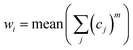
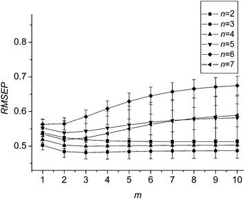
It is obvious that the weights (w) are key parameters to combine the sub-models for producing a satisfactory prediction. They reflect the relative importance of the sub-models in the combined model. The sub-model with big weight means a big contribution of the sub-model to the final prediction, and vice versa. As mentioned above, variables in sub-models are selected based on the rank of the stabilities. Since the stability of each variable shows its reliability for modeling, the sub-model built by the variables with higher stabilities should be given a bigger weight.

In order to assign an optimal weight for each sub-model, parameter m in (2) is investigated. A series of combined models are constructed with different number of sub-models, and used to predict the validation set, respectively. Fig. 1, 2(a) and 2(b) show the variation of the root mean square error of prediction (RMSEP) of the validation set along with the parameter m for prediction of starch, sugar and nicotine, respectively. It is clear that both figures show a similar variation trend. When m is 2, the RMSEPs reach at a minimum, and thereafter, the RMSEPs increase gradually. Thus m = 2 is used in this study.

Fig. 1 Variation of the mean RMSEPs and standard deviation with the value of parameter m for data set 1.

Fig. 2 Variation of the mean RMSEPs and standard deviation with the value of parameter m for data set 2 of sugar (a) and nicotine (b).

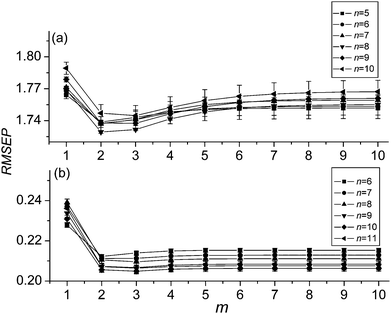
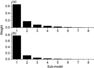
Moreover, with m = 2 and eight sub-models, the weights w of the sub-models for data set 1 is shown in Fig. 3. In the figure, it is obvious that the weights decrease along the order of the sub-models. The results mean that variables with big stabilities have large contributions to the model. This is consistent with the results obtained with the stability-based methods.^21–25 On the other hand, results in the figure also indicate that the variables with small stabilities also have contributions to the model, even relatively less than those variables with big stabilities. Therefore, VG-PLS, which uses all the variables, should have an advantage in prediction ability.

Fig. 3 Distribution of the weights of the sub-models for data set 1.

As for data set 2, the weights w of the sub-models for the sugar and nicotine are shown in Fig. 4(a) and (b), respectively. It can be seen that the distribution of weights for each sub-model is different from that of data set 1. In Fig. 4, it is obvious that the sub-model constructed by the first variable group has a big weight, the next three sub-models have relatively small weights, and other sub-models have very small weights. This may be accounted for by the large number of variables in data set 2, and the variables are sorted according to their importance to the model. Except the first four sub-models, the left sub-models mainly consist of the less relevant variables. This also indicates that reasonable weights are calculated for the sub-models, thus the prediction ability of the combined model can be improved with the advantage of using all the variables in the spectra.

Fig. 4 Distribution of the weights of the sub-models for data set 2 of sugar (a) and nicotine (b).

The number of sub-models

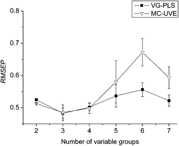
The number of sub-models (n) is also a key parameter in the proposed method. In order to investigate the influence of n on the prediction ability, the variation of the RMSEPs of the validation set versus the number of sub-models is investigated.

For data set 1, the variation of the RMSEPs of the validation set versus the number of sub-models is plotted in Fig. 5. Each point in the figure is the average value of the RMSEPs over 100 runs and the error bar across the points is the standard deviation (σ). From Fig. 5, it seems when n is 3, the RMSEP reaches the minimal. As a comparison, the variation of the RMSEP of the validation set for the data set by MC-UVE-PLS, where only the variables of the first sub-model are used, is also plotted in the figure. From the figure, it seems that when the number of sub-models is small, the mean value and the standard deviation of VG-PLS and MC-UVE are almost the same. When the number of sub-models increases, however, the mean value and the standard deviation of VG-PLS is obviously smaller than the results of MC-UVE. The result reveals that the model built by VG-PLS is improved with better stability than MC-UVE.

Fig. 5 Variation of the mean RMSEPs and standard deviation with different number of groups (n) for data set 1.

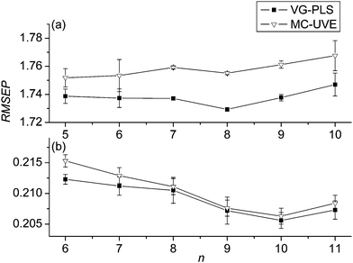
As in the same way done for data set 1, the variation of the RMSEPs of the validation set versus the number of sub-models for data set 2 is plotted in Fig. 6, in which (a) and (b) correspond to the sugar and nicotine, respectively. From Fig. 6(a), it appears that, at the beginning, both the mean value and the standard deviation are comparatively large. With the increase of n, however, the mean RMSEP decreases gradually and reaches a minimum at n = 8. This indicates that, when the combined model is built with 8 sub-models, the prediction ability of the model is best. Obviously, if fewer sub-models are built, e.g., 2 or 3, the advantage of grouping can not be seen because each group includes the variables with different stability. On the other hand, if more sub-models are used, fewer variables will be included in each sub-model, which may make the sub-models not predictable. Fig. 6(b) shows the variation of the RMSEPs of the validation set with the number of sub-models for the nicotine content of data set 2. It is clear that when n is 10, the RMSEP reaches a minimum. The number is slightly bigger than that in the sugar model, because the number of variables relevant to nicotine is relatively less compared with sugar.^23,25 Therefore, n = 8 and 10 is used as the number of sub-models for the sugar and nicotine model of data set 2.

Fig. 6 Variation of the mean RMSEPs and standard deviation with different number of groups (n) for data set 2 of sugar (a) and nicotine (b).

When compared with MC-UVE-PLS, it can be seen from the two curves in both Fig. 6(a) and (b) that the mean RMSEP of VG-PLS is slightly smaller than that of MC-UVE-PLS. The result reveals that, for data set 2, which is a data set of real complex samples, VG-PLS can obtain better results by making use of all variables with a suitable weighting strategy.

Distribution of the variables in sub-models

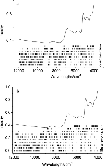
In order to further investigate the contribution of the variables in sub-models, the mean spectrum and the distribution of wavelengths in sub-models are plotted in Fig. 7 and 8 for the two data sets, respectively. In the figures, the wavelengths in each sub-model are labeled with a vertical short bar. It appears that for data set 1, the variables in the first group, which have main contribution to the model, are located in eight regions, and the two broad regions lie in the wavelength 4000–6000 cm⁻¹. Although it is generally difficult to interpret an NIR spectrum with chemical structure, these wavelengths correspond well with the NIR spectrum of starch, containing the first overtone and the combinations of O–H around 7000 and 5000 cm⁻¹.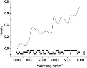

Fig. 7 The mean spectrum of calibration set and the wavelengths distribution in different groups for data set 1.

Fig. 8 The mean spectrum of calibration set and the wavelengths distribution in different groups for data set 2 of sugar (a) and nicotine (b).

Fig. 8(a) and (b) show the mean spectrum of the calibration set and the distribution of the wavelengths in different groups for data set 2 of the sugar and nicotine model, respectively. Due to the complexity of the samples and the large number of groups, the distribution seems complicated. However, for both the two models, the variables in the first group are mainly located in 4000–6000 cm⁻¹.This result has good consistency with that obtained in our previous works by using MC-UVE²⁵ and RT²⁸ methods. Therefore, there is no essential difference between the wavelength selection and the variable grouping strategies. The former uses only the variables which are considered to be important, and the latter adjust the importance of the variables by the weights.

Predictive validation

For data set 1, with n = 3, the RMSEPs of the prediction set (15 samples) for predicting the starch content by using the VG-PLS model are summarized in Table 1. For data set 2, with n = 8 and 10, respectively, the RMSEPs of the prediction set (549 samples) for predicting the sugar and nicotine contents by using the VG-PLS model are summarized in the table too. In Table 1, the mean RMSEPs and their standard deviation (σ) over 100 independent runs are listed. As comparisons, the mean RMSEPs obtained by ordinary PLS and MC-UVE-PLS using the raw and preprocessed spectra are also listed. From the table, it is clear that MSC can improve the prediction, and as a wavelength selection method, MC-UVE produces better prediction than the ordinary PLS. However, the efficiency of VG-PLS seems superior to MC-UVE-PLS, e.g., for data set 1, the mean RMSEP of VG-PLS is as small as that of MC-UVE-PLS, while the standard deviation of VG-PLS is smaller than that of MC-UVE-PLS. For data set 2, both the mean RMSEP and the standard deviation are improved by VG-PLS. Such results indicate that both the predictive ability and the stability of the model can be improved by using the weighted combined model.

Table 1 A comparison of the results obtained by different models

Data set	Contents	Model	Number of groups	Latent variables number (LV)	RMSEP(σ)^a
a RMSEP is the average value and σ is the standard deviation of the 100 RMSEPs. The RMSEP without σ is calculated with only one run because no stochastic factor is involved in the algorithms. b MC-UVE-1 means the MC-UVE reported in literature^25 and the number of retained variables is found by searching the minimal RMSEPs at different number of variables, whereas in MC-UVE-2, the same variables as in the first sub-model of VG-PLS is used for comparison. v is the number of retained wavelengths by MC-UVE.
1	Starch	PLS	1	6	1.142
		MSC + PLS	1	6	0.552
		MSC + MC-UVE-1^b (v = 236)	1	6	0.515 (0.049)
		MSC + MC-UVE-2 (v = 233)	1	6	0.520 (0.041)
		MSC + VG-PLS	3	6 6 5	0.535 (0.029)
2	Sugar	PLS	1	13	1.99
		MSC + PLS	1	13	1.71
		MSC + MC-UVE-1^b (v = 360)	1	13	1.61 (0.0056)
		MSC + MC-UVE-2 (v = 259)	1	13	1.63 (0.0019)
		MSC + VG-PLS	8	13 12 11 10 10 8 8 7	1.60 (0.0009)
	Nicotine	PLS	1	13	0.312
		MSC + PLS	1	13	0.303
		MSC + MC-UVE-1 (v = 215)	1	13	0.290 (0.0012)
		MSC + MC-UVE-2 (v = 207)	1	13	0.291 (0.0013)
		MSC + VG-PLS	10	13 13 13 12 10 8 8 7 7 7	0.290 (0.0012)

---

Conclusions

A combined model with new variable grouping strategy is proposed and applied to the modeling of NIR spectra of complex samples. The NIR spectra are split into different variable groups representing different spectral information based on stability, then sub-models are constructed by the grouped variables, and a combined model is finally built by a weighted combination of the sub-models. The proposed method is different from the variable selection methods, in which only the important variables are used, it makes a full use of the variables in NIR spectra for modeling. With two NIR data sets of corn and tobacco lamina samples, it was proved that the proposed method can effectively utilize all the variables with a suitable weighting for building a high performance PLS model.

Acknowledgements

This study was supported by National Natural Science Foundation of China (Nos. 20775036 and 20835002), and International Science and Technology Cooperation Program of the Ministry of Science and Technology (MOST) of China (No. 2008DFA32250).

References

1. J. Fontaine, B. Schirmer and J. Horr, J. Agric. Food Chem., 2002, 50, 3902.
2. K. Murayama, K. Yamada, R. Tsenkova, Y. Wang and Y. Ozaki, Vib. Spectrosc., 1998, 18, 33.
3. R. Marbach, T. H. Koschinsky, F. A. Gries and H. M. Heise, Appl. Spectrosc., 1993, 47, 875.
4. F. X. Wang, Z. Y. Zhang, X. J. Cui and P. de B. Harrington, Talanta, 2006, 70, 1170.
5. J. Luypaert, D. L. Massart and Y. Vander Heyden, Talanta, 2007, 72, 865.
6. W. Lindberg, J. A. Persson and S. Wold, Anal. Chem., 1983, 55, 643.
7. P. Dardenne, G. Sinnaeve and V. Baeten, J. Near Infrared Spectrosc., 2000, 8, 229.
8. M. Daszykowski, M. S. Wrobel, H. Czarnik-Matusewicz and B. Walczak, Analyst, 2008, 133, 1523.
9. P. Geladi, D. MacDougall and H. Martens, Appl. Spectrosc., 1985, 39, 491.
10. C. Pizarro, I. Esteban-Diez, A. J. Nistal and J. M. Gonzalez-Saiz, Anal. Chim. Acta, 2004, 509, 217.
11. R. J. Barnes, M. S. Dhanoa and S. J. Lister, Appl. Spectrosc., 1989, 43, 772.
12. Q. Guo, W. Wu and D. L. Massart, Anal. Chim. Acta, 1999, 382, 87.
13. N. A. Woody, R. N. Feudale, A. J. Myles and S. D. Brown, Anal. Chem., 2004, 76, 2595.
14. X. G. Shao, A. K. M. Leung and F. T. Chau, Acc. Chem. Res., 2003, 36, 276.
15. B. K. Alsberg, A. M. Woodward and D. B. Kell, Chemom. Intell. Lab. Syst., 1997, 37, 215.
16. D. Chen, F. Wang, X. G. Shao and Q. D. Su, Analyst, 2003, 128, 1200.
17. C. X. Ma and X. G. Shao, J. Chem. Inf. Comput. Sci., 2004, 44, 907.
18. D. Chen, W. S. Cai and X. G. Shao, Anal. Bioanal. Chem., 2007, 387, 1041.
19. R. Leardi and A. L. Gonzalez, Chemom. Intell. Lab. Syst., 1998, 41, 195.
20. L. Xu and W. J. Zhang, Anal. Chim. Acta, 2001, 446, 475.
21. V. Centner, D. L. Massart, O. E. de Noord, S. de Jong, B. M. Vandeginste and C. Sterna, Anal. Chem., 1996, 68, 3851.
22. J. Koshoubu, T. Iwata and S. Minami, Anal. Sci., 2001, 17, 319.
23. X. G. Shao, F. Wang, D. Chen and Q. D. Su, Anal. Bioanal. Chem., 2004, 378, 1382.
24. D. Chen, W. S. Cai and X. G. Shao, Anal. Chim. Acta, 2007, 598, 19.
25. W. S. Cai, Y. K. Li and X. G. Shao, Chemom. Intell. Lab. Syst., 2008, 90, 188.
26. L. Norgaard, A. Saudland, J. Wagner, J. P. Nielsen, L. Munck and S. B. Engelsen, Appl. Spectrosc., 2000, 54, 413.
27. S. D. Osborne, R. B. Jordan and R. Kunnemeyer, Analyst, 1997, 122, 1531.
28. H. Xu, Z. C. Liu, W. S. Cai and X. G. Shao, Chemom. Intell. Lab. Syst., 2009, 97, 189.
29. B. K. Alsberg, D. B. Kell and R. Goodacre, Anal. Chem., 1998, 70, 4126.
30. Z. C. Liu, W. S. Cai and X. G. Shao, Analyst, 2009, 134, 261.
31. L. Xu, J. H. Jiang, Y. P. Zhou, H. L. Wu, G. L. Shen and R. Q. Yu, Chemom. Intell. Lab. Syst., 2007, 87, 226.
32. H. W. Tan and S. D. Brown, J. Chemom., 2003, 17, 111.
33. R. W. Kennard and L. A. Stone, Technometrics, 1969, 11, 137.
34. D. W. Osten, J. Chemom., 1988, 2, 39.

---