Application of successive projections algorithm (SPA) as a variable selection in a QSPR study to predict the octanol/water partition coefficients (K_ow) of some halogenated organic compounds

Abstract

The successive projections algorithm (SPA) is a variable selection method that has been compared with the genetic algorithm (GA) due to its ability to solve the descriptor selection problems in QSPR model development. For model development, the popular linear algorithm Partial Least Squares (PLS) was employed to build the model. These methods were used for the prediction of octanol/water partition coefficients K_ow of 10 kinds of selected halogen benzoic acids. The root means square error of prediction (RMSEP) for training and prediction sets by GA-PLS and SPA-PLS models were 0.26, 0.28, 0.13 and 0.16, respectively. Also, the relative standard error of prediction (RSEP) for training and prediction sets by GA-PLS and SPA-PLS models were 8.02, 3.92, 8.68 and 4.98 respectively. The resultant data showed that SPA-PLS produced better results than GA-PLS in these class compounds.

---

1. Introduction

Halogenated benzoic acids are widespread environmental pollutants resulting primarily from production and use of xenobiotics. Two significant environmental sources of chlorinated benzoic acids are the microbial metabolism of herbicides and polychlorinated biphenyls.¹

Benzoic acid derivatives having a general structure C6–C1 are widely used as industrial chemicals, agrochemicals, pharmaceuticals and consumer products. On the other hand, a number of benzoic acid derivatives with variations including hydroxylation and methoxylation are known to be a group of secondary plant metabolites and also aerobic microbial degradation products of lignin, an important plant cell wall polymer.² Some of these naturally occurring benzoic acid derivatives are shown to have a range of biological activities.³ Furthermore, significant environmental sources of benzoic acids are from the microbial metabolism of a variety of natural and anthropogenic aromatic compounds, since benzoic acid derivatives are very common structural units among the identified or estimated degradation products of aromatic compounds by aerobic microorganisms.^4,5 However, the toxic effects of stable degradation intermediates from aromatic compounds are not fully elucidated.

Numerous studies have been made on the antibacterial, antifungal, and antiviral activities of natural and synthetic phenolic compounds including various substituted benzoic acids.⁶ However, studies on the effects of benzoic acids, as well as other carboxylic acids, to aquatic organisms have been limited.⁷ Toxicity data for some halogenated benzoic acids in the bacteria, ciliate, daphnids and fish have been reported.^8,1 Recently, the toxicity of substituted phenols to Daphnia has been investigated by many researchers.^9–15

If a third substance is added to a system of two immiscible liquids in equilibrium, the added component will distribute itself between the two liquid phases until the ratio of its concentrations in each phase attains a certain value: the distribution constant or partition coefficient. The measurement of liquid–liquid partition coefficients is extremely important in: (1) fundamental chemistry for studying inorganic and/or organic complex equilibria; (2) industrial chemistry for optimization of production and waste treatment; and (3) food chemistry for purification and extraction of sugars, fat or caffeine.¹⁶ This field is so important that many universities offer a special course in liquid–liquid partitioning and solvent extraction. The n-octanol–water partition coefficient (K_ow) is the ratio of the concentration of a chemical in n-octanol to that in water in a two-phase system at equilibrium. The logarithm of this coefficient, log K_ow, has been shown to be one of the key parameters in quantitative structure–activity/property relationship (QSAR/QSPR) studies. On the other hand, the octanol–water partition coefficient can be defined as a parameter that measures the hydrophobicity of a substance. Hydrophobic interactions are of critical importance in many areas of chemistry, including enzyme–ligand interactions, drug–receptor interactions, transport of drug to the active site, the assembly of lipids in biomembranes, aggregation of surfactants, coagulation, and detergency, etc.^17,18 Experimental determination of log K_ow is often complex and time-consuming and can be done only for already synthesized compounds. For this reason, a number of computational methods for the prediction of this parameter have been proposed.

In recent years, several QSPR models based on both linear and nonlinear methods that aimed to predict the partition coefficient and other physiochemical properties were developed.^19–30 However, many of these studies tended to focus more on the modeling ability of the QSPR models and paid little consideration to model validation and applicability which is essential for the assessment of the reliability. Altogether they have used nonlinear methods when they could obtain the best result with linear methods. In QSAR/QSPR studies two considerations are very important, the first is the descriptors to ensure that they carry enough information of molecular structure for the interpretation of the activity property, the second is the modeling method employed.³¹ In this investigation, we used SPA (successive projections algorithm) for feature selection, which is a forward selection method that starts with one variable, and then incorporates a new one at each iteration, until a specified number N of variables is reached. SPA is a technique specifically designed to select subsets of variables with small collinearity and to improve the conditioning of Multiple Linear Regression (MLR) models. This algorithm was originally proposed for wavelength selection in spectroscopic data sets, especially under conditions of strong spectral overlapping.³² MLR models obtained by using SPA have been shown to be superior, in terms of prediction ability, to full-spectrum PLS (Partial Least Squares) models in a variety of applications, including UV–VIS,^32–35 ICP–OES,³⁶ FT–IR³⁷ and NIR spectrometry.^38,39 SPA has also been successfully employed to various classification studies.^40,41

SPA includes three phases.⁴² At first, the algorithm builds candidate subsets of variables on the basis of a collinearity minimization criterion. Such subsets are built according to a sequence of vector projection operations applied to the columns of the matrix of available predictor data. In the second phase, the best candidate subset is chosen based on minimum root mean square error (RMSE) obtained in a validation set.⁴³ And finally, the selected subset is subjected to an elimination procedure to determine if any variables can be removed without significant loss of prediction ability.

Each of these phases is explained in detail elsewhere.⁴⁴

Although SPA was initially designed for use with MLR models, it may be worth investigating whether it could be employed with different modeling techniques. In our previous work we used SPA as selection variable method and MLR and Artificial Neural Network (ANN) techniques to build models.²⁵ Note that, genetic algorithms are random search techniques inspired by natural selection mechanisms, which explore a complex solution space in an efficient manner. However, due to their stochastic nature, results are realization dependent and variable selections may not be reproducible (especially for data sets involving a large number of variables). SPA, as a forward selection method based on minimum collinearity between the introduced variables, is able to be compared with GAs in many applications.⁴⁵

SPA starts with one variable, and then includes a new one at each epoch, until a specified number, N, of a variable is reached. SPA steps are described below, assuming that the first variable, k(0), and the number N are given.

Step 0: Before the first iteration (n = 1), let X_j = jth column of Xcal; j = 1,…, J

Step 1: Let S be the set of variables which have not been selected yet. That is, S = {J such that 1 ≤ j ≤ J and j ∉ {k(0),…,k(n − 1)}}

Step 2: Calculate the projection of X_j on the subspace orthogonal to X_k(n-1) as:

Px_j = x_j − (x^T_jx_k(n−1))x_k(n−1)(x^T_{k(n − 1)}|x_k(n−1))⁻¹

for all j ∈ S, where P is the projection operator.

Step 3: Let k(n) = arg(max‖Px_j‖,j ∈ S

Step 4: Let x_j = Px_j,j ∈ S

Step 5: Let n = n + 1. if n < N go back to step 1.

End: The resulting variables are {k(n); n = 0,…,N−1}

The number of projection operations performed in the selection process can be shown to be (N−1) (J−N/2).

Its purpose is to select variables whose information content is minimally redundant, in order to solve collinearity problems^46–48 in a feature selection procedure that has been compared with GAs, due to its ability to solve the descriptor selection problems in QSPR model development. For model development, a popular linear algorithm PLS was employed to build model.

2. Materials and methods

2.1 Data set

Experimental octanol–water partition coefficients (K_ow) data of some substituted benzene derivatives containing halogens and carboxyls compounds were taken from [49]. Several review articles describing the various methods used to determine liquid–liquid partition coefficients and especially K_ow appeared recently.^50–52 The names of these compounds and their experimental and calculated octanol-water partition coefficients by GA–PLS and SPA–PLS methods are shown in Table 1. As can be seen, this set contains in total 57 octanol-water partition coefficients data. The octanol–water partition coefficient values for these compounds were obtained in the same instrumental conditions.

Table 1 Data set and corresponding observed and predicted values of the octanol-water partition coefficients

No.	Compounds	Exp.	GA–PLS	SPA–PLS
a The compounds used for prediction set.
1^a	Chlorobenzene	2.84	3.19	2.83
2	Iodobenzene	3.25	3.35	3.30
3	Bromobenzene	2.99	3.08	3.05
4	Fluorobenzene	2.27	2.20	2.30
5	o-Dibromobenzene	3.64	3.82	3.58
6	m-Dibromobenzene	3.75	3.76	3.77
7	p-Dibromobenzene	3.79	3.86	4.01
8	m-Dichlorobenzene	3.53	3.58	3.42
9	o-Dichlorobenzene	3.43	3.45	3.39
10	p-Dichlorobenzene	3.44	3.49	3.40
11	m-Difluorobenzene	2.21	2.32	2.32
12	o-Difluorobenzene	2.37	2.36	2.38
13	p-Difluorobenzene	2.13	2.31	2.28
14	p-Diiodobenzene	4.11	4.16	4.02
15	1,2,3-Trichlorobenzene	4.05	3.94	3.95
16	1,2,4-Trichlorobenzene	4.02	4.05	3.99
17^a	1,3,5-Trichlorobenzene	4.19	4.51	4.02
18	1,3,5-Tribromobenzene	4.51	4.03	4.48
19	1,2,4-Trifluorobenzene	2.52	2.41	2.40
20	1,2,4,5-Tetrabromobenzene	5.13	5.30	5.19
21	1,2,3,4-Tetrachlorobenzene	4.6	4.57	4.54
22	1,2,3,5-Tetrachlorobenzene	4.56	4.60	4.57
23	1,2,4,5-Tetrachlorobenzene	4.64	4.65	4.63
24^a	Pentachlorobenzene	5.17	5.37	5.22
25	Pentafluorobenzene	2.53	2.53	2.50
26	Hexachlorobenzene	5.73	5.82	5.70
27	Hexabromobenzene	6.07	5.77	6.20
28	Hexafluorobenzene	2.55	2.47	2.47
29	Benzoic acid	1.87	1.90	1.83
30	o-Chlorobenzoic acid	2.05	2.01	2.07
31^a	m-Chlorobenzoic acid	2.68	2.92	2.43
32	p-Chlorobenzoic acid	2.65	2.64	2.68
33	o-Bromobenzoic acid	2.2	1.97	2.09
34	m-Bromobenzoic acid	2.87	2.86	2.95
35	p-Bromobenzoic acid	2.86	2.79	2.77
36	o-Fluorobenzoic acid	1.77	1.75	1.62
37^a	m-Fluorobenzoic acid	2.15	1.90	1.92
38	p-Fluorobenzoic acid	2.07	2.10	2.11
39	o-Iodobenzoic acid	2.4	2.22	2.27
40^a	m-Iodobenzoic acid	3.13	2.80	3.19
41	p-Iodobenzoic acid	3.02	2.91	2.92
42	2,5-Dichlorobenzoic acid	2.82	2.92	2.74
43	2,6-Dichlorobenzoic acid	2.23	2.22	2.44
44	3,4-Dichlorobenzoic acid	3.25	3.33	3.32
45	3,5-Dichlorobenzoic acid	3.00	3.52	2.91
46	2,6-Difluorobenzoic acid	1.59	1.72	1.54
47	2-Chloro-6-Fluorobenzoic acid	2.11	2.01	1.98
48	2-Chloro-3-Fluorobenzoic acid	1.74	2.25	2.03
49	4-Chloro-2-Fluorobenzoic acid	2.28	2.54	2.51
50^a	2-Bromo-5-Fluorobenzoic acid	2.21	2.55	2.49
51	3-Bromo-4-Fluorobenzoic acid	3.56	2.99	3.30
52	2-Fluoro-4-Bromobenzoic acid	2.76	2.68	2.52
53	2-Fluoro-5-Chlorobenzoic acid	1.59	2.50	2.02
54	2-Chloro-4-Fluorobenzoic acid	2.63	2.24	2.61
55^a	2-Chloro-5-Fluorobenzoic acid	2.39	2.07	2.31
56^a	2-Chloro-5-Bromobenzoic acid	3.16	3.09	3.14
57	2-Fluoro-5-Bromobenzoic acid	3.43	2.58	3.49

---

2.2 Descriptor generation and screening

The octanol–water partition coefficients (K_ow) of solutes in separation methods are related to some structural, electronic and geometric properties of solutes. The value of these molecular features can be encoded quantitatively by numerical values named molecular descriptors. These molecular parameters are to be used to search for the best QSPR model of octanol-water partition coefficients. The 2D structures of the molecules were drawn using (Hyperchem 7 software).⁵³ These were pre-optimized with Molecular Mechanics Force Field (MM+) and final geometries were obtained with the semi-empirical AM1 method in the Hyperchem program. All calculations were carried out at the restricted Hartree–Fock level with no configuration interaction. The molecular structures were optimized using the Polak–Ribiere algorithm until the root mean square gradient was 0.001 Kcal mol⁻¹. The resulting geometry was transferred into the Dragon program package, which was developed by Milano chemometrics and QSPR group⁵⁴ to calculate about 1457 descriptors in constitutional, topological, geometrical, charge, GETAWAY (Geometry, Topology and Atoms-Weighted Assembly), WHIM (Weighted Holistic Invariant Molecular descriptors), 3D-MoRSE (3D-Molecular Representation of Structure based on Electron diffraction), molecular walk count, BCUT, 2D-autocorrelation, aromaticity index, randic molecular profile, radial distribution function, functional group and atom-centered fragment classes. The 1457 descriptors were first analyzed for the existence of constant or near constant variables. The detected ones were then removed leaving 650 descriptors, as too many included zero values and did not have any information on structures. Secondly, correlation among descriptors and the log K_o/w of the molecules was examined and collinear descriptors (i.e. correlation coefficient between descriptors is greater than 0.9) were detected. Descriptors that contain a high percentage (>90%) of identical values for all the 57 molecules were discarded to decrease the redundancy in the descriptor data matrix. Among the collinear descriptors, the one presenting the highest correlation with the log K_ow to be predicted was retained and others were removed from the data matrix. At the end 263 descriptors remained. The Hyperchem output files were used by the Gaussian 98 program⁵⁵ to calculate 2 classes of descriptor: electrostatic (minimum and maximum of partial charge, polarity parameters, charge surface area descriptors, etc.) and quantum chemical (Dipole moment, HOMO and LUMO energies, etc.). This was operated to be optimized with 6–31⁺G^** basis set for all atoms at the B3LYP level.^56,57 No molecular symmetry constraint was applied, rather full optimization of all bond lengths and angles was carried out at the level B3LYP/6-31⁺⁺G^**. It should be noted that we obtained 13 descriptors using the Gaussian program, which we added to the 263 descriptors that were obtained from Dragon descriptors. Table 2 shows all information about descriptors were selected by GA and SPA. To demonstrate the absence of chance correlations on the best models obtained with the above procedure, we performed a Y-scrambling test, where the output values of the compounds were shuffled randomly, and the scrambled data set was re-examined by the PLS method against real (unscrambled) input descriptors to determine the correlation and predictivity of the resulting model. The correlation coefficient results were 0.093 (±0.022) and 0.113 (±0.011) for SPA and GA (in 30 repetitions), respectively. Therefore the results show that there is no chance of correlation in models with the selected descriptors using both methods.

Table 2 Descriptors and their definitions were selected by GA and SPA

Descriptors were selected by GA	Definition	Descriptors were selected by SPA	Definition
BEHp7	Highest eigenvalue n.7 of Burden matrix/ weighted by atomic polarizabilities	Mor26u	3D MoRSE-signal26/ unweighted
ATS4e	Broto-Moreau autocorrelation of a topological structure-lag4/ weighted by atomic Sanderson electronegativities	TIE	E-state topological parameter
RDF050u	Radial Distribution function-5.0/ unweighted	H2v	H autocorrelation of lag2/ weighted by atomic van der Waals volumes
Mor06u	3D MoRSE-signal06/ unweighted	MATS5m	Moran autocorrelation-lag 5/ weighted by atomic masses
Mor31e	3D MoRSE-signal31/ weighted by atomic Sanderson electronegativities	ATS5e	Broto-Moreau autocorrelation of a topological structure-lag5/ weighted by atomic Sanderson electronegativities
E1v	First component accessibility directional WHIM index/ weighted by atomic van der Waals volumes	RDF065e	Radial Distribution function-6.5/ weighted by atomic Sanderson electronegativities
R4e	R autocorrelation of lag4/ weighted by atomic Sanderson electronegativities	RDF060m	Radial Distribution function-6.0/ weighted by atomic masses

---

4. Results and discussion

Although traditional methods or network-based techniques play an important role in QSPR studies, the success of a study depends also on the selection of variables (molecular descriptors).⁵⁸ In order to make feasible the building of the PLS model, techniques of variable selection GA and SPA, were applied to the data. As is mentioned above, SPA is an iterative forward selection method that operates on the response matrix, whose lines and columns correspond to calibration samples and variables, respectively. Generally, the prediction ability of QSAR/QSPR models is affected by two factors. One is the descriptors, which should carry enough information of molecular structure for the interpretation of the activity/property. The other is the modeling method employed.⁵⁸ The number of descriptors available for QSAR/QSPR studies is often so large that it is difficult to obtain a model including all of them. Therefore identifying important descriptors certainly plays an important role in QSAR/QSPR. Descriptors should represent the maximum information in activity variations and collinearity among them must be kept to a minimum. Among different feature selection strategies, genetic algorithms are an interesting, flexible and widely used alternative.⁵⁹ The resulting selected variables are reproducible for different runs of SPA. Table 2 and 3; introduce the correlation coefficient matrix between the descriptors that have been selected by SPA and GA, respectively. These two tables show that there is not significant correlation between the selected descriptors. Obviously, high correlation (>0.9) between the descriptors is indicative of collinearity, and so this is not a problem for our models. When constructing a model, we used descriptors with low correlations, because molecular descriptors are independent variables. Correlation matrix for these descriptors is shown in Table 3 and Table 4.

Table 3 Correlation matrix for the seven selected descriptors using SPA method

	Mor26u	TIE	H2v	MATS5m	ATS5e	RDF065e	RDF060m
Mor26u	1
TIE	0.2375	1
H2v	0.0086	0.1291	1
MATS5m	0.0725	0.0531	0.6234	1
ATS5e	0.3189	0.0084	0.0732	0.1662	1
RDF065e	0.0018	0.0005	0.0624	0.0056	0.1754	1
RDF060m	0.023	0.0005	0.0013	0.0033	0.1188	0.0003	1

---

Table 4 Correlation matrix for the seven selected descriptors using GA method

	BEHp7	ATS4e	RDF050u	Mor06u	Mor31e	E1v	R4e
BEHp7	1
ATS4e	0.5594	1
RDF050u	0.2867	0.2356	1
Mor06u	0.0001	0.0674	0.3565	1
Mor31e	0.2647	0.0761	0.0232	0.4564	1
E1v	0.0015	0.2961	0.0039	0.1004	0.0075	1
R4e	0.2980	0.8995	0.0945	0.0434	0.043	0.4493	1

---

The great interest in QSPR model establishment is the determination of the relevant variables that best describe dependencies between activity (and property) and chemical structures of compounds. More often than not, interrelation between variables skews the results, and therefore, fortuitous or artificial QSPR models may be obtained. In some of the previous studies, the selection of variables for an eventual nonlinear model has been performed using a linear model such as MLR.^32,60 In this work, PLS as a linear modeling tool was applied.⁶¹

One of the important phases of PLS is to select the best latent variables, which are effective for the model and must be selected based on Q² of cross-validation or RMSEC/RMSECV to prevent underfitting or overfitting. In this study the optimum number of factors (latent variables) to be included in the calibration model was determined by computing the root mean squares of error of calibration set (RMSEC) and validation set (RSMECV) for GA–PLS and SPA-PLS. Fig. 1 shows the variation of RMSEC/RSMECV with the number of components for these methods. As can be see from this figure, the optimum numbers of components for GA–PLS and SPA–PLS methods are 4 and 5 respectively. When the latent variables are similar to each other or it is uncertain which the best are, one reasonable choice for the optimum number of factors would be that number which yielded the minimum RMSEC/RSMECV. Since there are a finite number of compounds in the training set, in many cases the minimum RMSEC/RSMECV value causes overfitting or underfitting for unknown compounds that were not included in the model.

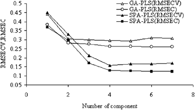Fig. 1 Plots of the RMSECV/RMSEC vs. number of compounds by SPA-PLS and GA-PLS.

A solution to this problem has been suggested^62,63 in which the RMSE values for all previous factors are compared to the RMSE value at the minimum. The F-Statistical test can be used to determine the significance of RMSE values greater than the minimum. In all instances, the number of factors for the first RMSE values whose F-ratio probability drops below 0.75 was selected as the optimum value. The GA selection process proceeded with an initial population of 30 solutions (chromosomes), probability of mutation 1% and 100 iterations, crossover probability 0.6. Fig. 2 shows the plot of the GA–PLS predicted against the experimental values of octanol–water partition coefficients (K_o/w) for the molecules included in the data set.

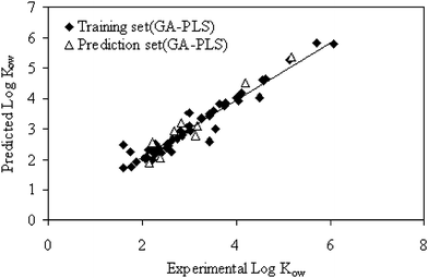Fig. 2 Plot of calculated octanol-water partition coefficients vs. experimental values for GA-PLS method.

Fig. 3 shows the propagation of residuals at both sides of the zero line, which are plotted as experimental values versus the residuals using the GA–PLS. The SPA–PLS predicted octanol–water partition coefficients (K_o/w) are plotted against experimental values in Fig. 4. Also, the residuals of the SPA–PLS calculated values of octanol–water partition coefficients are plotted against the experimental values in Fig. 5. These plots illustrate that SPA–PLS is a powerful technique for the prediction of octanol–water partition coefficients. On the other hand, from Fig. 3 and Fig. 5, it can be seen that there is no systematic error for these models.

Fig. 3 Plot of the residuals vs. experimental values for GA–PLS method.

Fig. 4 Plot of calculated octanol–water partition coefficients vs. experimental values for SPA–PLS method.

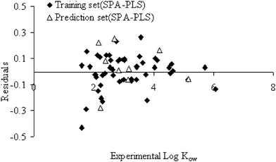Fig. 5 Plot of the residuals vs. experimental values for SPA–PLS method.

WHIM descriptors are one of the descriptors which were used in the models. WHIM descriptors are molecular descriptors based on statistical indices calculated on the projection of the atoms along principal axes. These descriptors are built in such a way as to capture relevant molecular 3D information regarding molecular size, shape, and symmetry and atom distribution with respect to invariant reference frames. The algorithm consists of performing a principal component analysis on the centered Cartesian coordinates of molecules by using weighted covariance matrix obtained from different weighting schemes for atoms:

Where S_jk is the weighted covariance between the j th and k th atomic coordinates, A is the number of atoms, w_i the weight of the ith atom, q_ij and q_jk represent the j th and k th coordinate (j,k = x,y,z) of the ith atom respectively and q̄ the corresponding average value.

The second type of descriptor which was used in this study is Moreau-Broto autocorrelation. This is a spatial autocorrelation defined on a molecular graph G as:

where w is any atomic property, A is the atom number, d is the considered topological distance (i.e., the lag in autocorrelation terms) ξ_ij is Kronecker delta (ξ_ij = 1 if dimensional vector) of atomic properties.

The other descriptors used in the models are called 3D-MoRSE descriptors. These types of descriptors are based on the idea of obtaining information from the 3D atomic coordinates by the transform used in electron diffraction studies for preparing theoretical scattering curves. A generalized scattering function, called the molecular transform, can be used as the functional basis for deriving from a known molecular structure, the specific analytical relationship of both X-ray and electron diffraction. The general molecular transform is:

where S represents the scattering in various directions by a collection of A atoms located at points r_i; f_i is a form factor taking into account the direction dependence of scattering from a spherical body of finite size. The scattering value S measures the scattering angle as:

S = 4Π·sin(ϑ/2)/λ

where ϑ and λ are the scattering angle the wavelength of the electron beam respectively.

The BCUT metrics are extensions of parameters originally developed by Burden.⁶⁴ The Burden parameters are based on a combination of the atomic number for each atom and a description of the nominal bond-type for adjacent and nonadjacent atoms. The BCUT metrics expand the number and types of atomic features that can be considered and also provide a greater variety of proximity measures and weighting schemes. The result is a new, whole-molecule descriptor that has shown significant utility in the measurement of molecular diversity and related tasks.

Radial distribution function (RDF) descriptors are based on the distance distribution in the geometrical representation of a molecule and constitute a RDF that shows certain characteristics in common with the 3D-MORSE descriptors. Formally, the radial distribution function of an ensemble of an atom can be interpreted as the probability distribution of finding an atom in a spherical volume of radius R. The general form of the radial distribution function is shown as:

where f is a scaling factor, w are characteristic atomic properties of the atoms i and j, r_ij are the interatomic distances between the i th and j th atoms, respectively, and A is the number of atoms. The exponential term contains the distance r_ij between the atoms i and j and the smoothing parameter g, which defines the probability distribution of the individual interatomic distance; it can be interpreted as a temperature factor that defines the movement of atoms. g(R) is generally calculated at a number of discrete points with defined intervals. However, these atomic properties enable the discrimination of the atoms of a molecule for almost any property that can be attributed to an atom.

Other descriptors include so called GETAWAY descriptors. GETAWAY descriptors are calculated from the leverage matrix obtained by the centered atomic coordinates molecular influence matrix (MIM). The first four descriptors are calculated as information content and connectivity indices. HATS and H descriptors are 3D autocorrelation descriptors obtained from MIM; R and R+ descriptors are analogously obtained from the leverage/geometry matrix. Descriptors appearing in these QSPR models provide information related to different molecular properties, which can participate in the physicochemical process that affected the logarithmic n-octanol/water partition coefficient of the solutes. The statistical parameters for GA-PLS and SPA-PLS methods are shown in Table 5. These parameters are NCP, RMSEC, RSMECV, Q2 LOO, RMSEP, RSEP%, MAE% and R2. The results show that both models were achieved in this study but SPA-PLS was more reliable in predicting the n-octanol-water partition coefficients of some substituted benzene derivatives containing halogens and carboxyl compounds.

Table 5 Statistical parameters for SPA-PLS and GA-PLS models

Parameters		SPA-PLS	GA-PLS
a Number of components. b Q^2 Leave one out cross-validation.
NOC (LV)^a		4	5
RMSECv		0.16	0.29
RMSEC		0.13	0.26
Q^2 LOO^b		0.91	0.92
RMSEP	Training set	0.13	0.26
	Prediction set	0.16	0.28
RSEP(%)	Training set	3.92	8.02
	Prediction set	4.98	8.68
MAE(%)	Training set	4.48	5.78
	Prediction set	11.93	17.25
R^2	Training set	0.98	0.94
	Prediction set	0.97	0.94
Fstatistical	Training set	3073.98	701.18
	Prediction set	257.93	106.16
Ttest	Training set	55.44	26.48
	Prediction set	16.06	10.30

---

5. Conclusion

GA–PLS and SPA–PLS were used as feature mapping techniques for the prediction of octanol–water partition coefficients of some substituted benzene derivatives containing halogens and carboxyl compounds. The results obtained reveal the superiority of SPA–PLS over the GA–PLS models. This is due to the ability of SPA–PLS to allow for flexible mapping of the selected features by manipulating their functional dependence implicitly, unlike regression analysis. Relations between the different molecular properties and the octanol-water partition coefficients is possible by using the descriptors that appeared in these QSPR models.

Acknowledgements

This work was supported by the research grant from Shahrood University of Technology.

References

1. M. Muccini, A. C. Layton, G. S. Sayler and T. W. Schultz, Bull. Environ. Contam. Toxicol., 1999, 62, 616.
2. C. L. Chen, H. M. Chang, Chemistry of lignin biodegradation. In: Higuchi, T. (Ed.), Biosynthesis and Biodegradation of Wood Components. Academic Press, Florida, ( 1985).
3. F. A. Tomas-Barberan and M. N. Clifford, J. Sci. Food Agric., 2000, 80, 1024.
4. M. R. Smith, Biodegradation, 1990, 1, 191.
5. H. Habe and T. Omori, Biosci., Biotechnol., Biochem., 2003, 67, 225.
6. M. Friedman, P. R. Henika and R. E. Mandrell, J. Food Protect, 2003, 66, 1811.
7. A. Fiorentino, A. Gentili, M. Ishidori, P. Monaco, A. Nardelli, A. Parrella and F. Temussi, J. Agric. Food Chem., 2003, 51, 1005.
8. Y. H. Zhao, X. Yuan, L. H. Yang and L. S. Wang, Bull. Environ. Contam. Toxicol., 1996, 57, 242.
9. J. Padmanabhan, R. Parthasarathi, V. Subramanian and P. K. Chattaraj, Chem. Res. Toxicol., 2006, 19, 356.
10. J. Devillers, Sci. Total Environ., 1988, 76, 79.
11. G. A. LeBlanc, Bull. Environ. Contam. Toxicol., 1980, 24, 684.
12. J. Devillers and P. Chambon, Bull. Environ. Contam. Toxicol., 1986, 37, 599.
13. R. Kuhn, M. Pattard, K. D. Pernak and A. Winter, Water Res., 1989, 23, 495.
14. L. Jin, J. Dai, P. Guo, L. Wang, Z. Wei and Z. Zhang, Chemosphere, 1998, 37, 79.
15. T. Abe, H. Saito, Y. Niikura, T. Shigeoka and Y. Nakano, Water Sci. Technol., 2000, 42, 297.
16. J. Rydberg, C. Musikas, G. R. Choppin, Principle and Practices of Solvent Extraction, Marcel Dekker, New York, 1992.
17. C. D. Selassie, D. J. Abraham, Burger's Medicinal Chemistry and Drug Discovery, Wiley, New Jersey, 2003.
18. R. Franke, Theoretical Drug Design Methods, Elsevier, Amsterdam, 1984.
19. N. Goudarzi, M. P. Freitas and T. C. Ramalho, Spectrochimica Acta Part A, 2009, 74, 563.
20. N. Goudarzi and M. Goodarzi, Mol. Phys., 2008, 106, 2525.
21. N. Goudarzi and M. Goodarzi, Mol. Phys., 2009, 107, 1739.
22. N. Goudarzi and M. Goodarzi, Mol. Phys., 2009, 107, 1787.
23. N. Goudarzi and M. Goodarzi, Mol. Phys., 2009, 107, 1495.
24. N. Goudarzi and M. Goodarzi, Mol. Phys., 2009, 107, 1615.
25. N. Goudarzi, M. Goodarzi, M. C. U. Araujo and R. K. H. Galvao, J. Agric. Food Chem., 2009, 57, 7153.
26. M. H. Fatemi and N. Goudarzi, Electrophoresis, 2005, 26, 2968.
27. W. Lu, Y. Chen, M. Liu, X. Chen and Z. Hu, Chemosphere, 2007, 69, 469.
28. M. H. Fatemi and F. Karimian, J. Colloid Interface Sci., 2007, 314, 665.
29. V. Tantishaiyakul, J. Pharm. Biomed. Anal., 2005, 37, 411.
30. N. Goudarzi, M. H. Fatemi and A. Samadi-Maybodi, Spectrosc. Lett., 2009, 42, 186.
31. M. Goodarzi and M. P. Freitas, QSAR Comb. Sci., 2008, 27, 1092.
32. M. C. U. Araujo, T. C. B. Saldanha, R. K. H. Galvão, T. Yoneyama, H. C. Chame and V. Visani, Chemom. Intell. Lab. Syst., 2001, 57, 65.
33. H. A. Dantas Filho, E. S. O. N. Souza, V. Visani, S. R. R. C. Barros, T. C. B. Saldanha, M. C. U. Araújo and R. K. H. Galvão, J. Braz. Chem. Soc., 2005, 16, 58.
34. M. S. Di Nezio, M. F. Pistonesi, W. D. Fragoso, M. J. C. Pontes, H. C. Goicoechea, M. C. U. Araújo and B. S. Fernandez Band, Microchem. J., 2007, 85, 194.
35. M. Grunhut, M. E. Centurión, W. D. Fragoso, L. F. Almeida, M. C. U. Araujo and B. S. F. Band, Talanta, 2008, 75, 950.
36. R. K. H. Galvão, M. F. Pimentel, M. C. U. Araujo, T. Yoneyama and V. Visani, Anal. Chim. Acta, 2001, 443, 107.
37. F. A. Honorato, R. K. H. Galvão, M. F. Pimentel, B. B. Neto, M. C. U. Araújo and F. R. Carvalho, Chemom. Intell. Lab. Syst., 2005, 76, 65.
38. M. C. Breitkreitz, I. M. Raimundo Jr., J. J. R. Rohwedder, C. Pasquini, H. A. Dantas Filho, G. E. José and M. C. U. Araújo, Analyst, 2003, 128, 1204.
39. H. A. D. Dantas Filho, R. K. H. Galvão, M. C. U. Araújo, E. C. Silva, T. C. B. Saldanha, G. E. José, C. Pasquini, I. M. Raimundo Jr. and J. J. R. Rohwedder, Chemom. Intell. Lab. Syst., 2004, 72, 83.
40. M. J. C. Pontes, R. K. H. Galvão, M. C. U. Araújo, P. N. T. Moreira, O. D. Pessoa Neto, G. E. José and T. C. B. Saldanha, Chemom. Intell. Lab. Syst., 2005, 78, 11.
41. F. F. Gambarra-Neto, G. Marino, M. C. U. Araújo, R. K. H. Galvão, M. J. C. Pontes, E. P. de Medeiros and R. S. Lima, Talanta, 2009, 77, 1660.
42. R. K. H. Galvão, M. C. U. Araújo, W. D. Fragoso, E. C. Silva, G. E. José, S. F. C. Soares and H. M. Paiva, Chemom. Intell. Lab. Syst., 2008, 92, 83.
43. R. K. H. Galvão, M. C. U. Araújo, E. C. Silva, G. E. José, S. F. C. Soares and H. M. Paiva, J. Braz. Chem. Soc., 2007, 18, 1580.
44. R. K. H. Galvão, M. C. U. Araújo, Linear Regression Modeling: Variable Selection. In: S. Brown, R. Tauler, B. Walczak, (Ed.) Comprehensive Chemometrics, Elsevier, 2009.
45. M. Kompany-Zareh and M. Mirzaei, Anal. Chim. Acta, 2004, 521, 231.
46. M. C. U. Araujo, T. C. B. Saldanha, R. K. H. Galvão, T. Yoneyama, H. C. Chame and V. Visani, Chemom. Intell. Lab. Syst., Lab. Inf. Manag., 2001, 57, 65.
47. Q. Guo, W. Wu, D. L. Massart, C. Boucon and S. de Jong, Chemom. Intell. Lab. Syst., 2002, 61, 123.
48. Y. Akhlaghi and M. Kompany-Zareh, J. Chemom., 2006, 20, 1.
49. Y. Qiao, S. Xia and P. Ma, J. Chem. Eng. Data, 2008, 53, 280.
50. J. Sangster, Octanol–Water Partition Coefficients, Fundamentals and Physical Chemistry, Wiley, Chichester, 1997.
51. S. K. Poole and C. F. Poole, J. Chromatogr., B: Anal. Technol. Biomed. Life Sci., 2003, 797, 3.
52. L. G. Danielsson and Y. H. Zhang, Trends Anal. Chem., 1996, 15, 188.
53. K. Valko, (Ed.), Separation Methods in Drug Synthesis and Purification, Elsevier, Amsterdam, 2000.
54. HyperChem., re. 4 for Windows; AutoDesk, Sausalito, CA, 1995.
55. R. Todeschini, Milano Chemometrics and QSPR Group, http://www.disat.unimib.it/vhml.
56. M. J. Frisch, G. W. Trucks, H. B. Schlegel, G. E. Scuseria, M. A. Robb, J. R. Cheeseman, V. G. Zakrzewski, J. A. Montgomery Jr., R. E. Stratmann, J. C. Burant, S. Dapprich, J. M. Millam, A. D. Daniels, K. N. Kudin, M. C. Strain, O. Franks, J. Tomasi, V. Barone, M. Cossi, R. Cammi, B. Mennucci, C. Pomelli, C. Adamo, S. Clifford, J. Ochterski, G. A. Petersson, P. Y. Ayala, Q. Cui, K. Morokuma, D. K. Malick, A. D. Rabuck, K. Raghavachari, J. B. Foresman, J. Cioslowski, J. V. Ortiz, B. B. Stefanov, G. Liu, A. Liashenko, P. Piskorz, I. Komaromi, R. Gomperts, R. L. Martin, D. J. Fox, T. Keith, M. A. Al-Laham, C. Y. Peng, A. Nanayakkara, C. Gonzalez, M. Challacombe, P. M. W. Gill, B. Johanson, W. Chen, M. W. Wong, J. L. Andres, C. Gonzalez, M. Head-Gordon, E. S. Replogle, J. A. Pople, Gaussian 03, Revision B.03, Gaussian Inc., Pittsburgh, PA ( 2003).
57. J. Padmanabhan, R. Parthasarathi, V. Subramanian and P. K. Chattaraj, Bioorg. Med. Chem., 2006, 14, 1021.
58. W. Zhou, Z. Zhai, Z. Wang and L. Wang, THEOCHEM, 2005, 755, 137.
59. J. Zupan and M., Anal. Chim. Acta, 1997, 348, 409.
60. M. Jalali-Heravi and F. Parastar, J. Chem. Inf. Comp. Sci, 2000, 40, 147.
61. L. Douali, D. Villemin and D. Cherqaoui, J. Chem. Inf. Comp. Sci, 2003, 43, 1200.
62. M. Goodarzi and M. P. Freitas, J. Phys. Chem. A, 2008, 112, 11263.
63. M. Goodarzi, T. Goodarzi and N. Ghasemi, Ann. Chim., 2007, 97, 303.
64. F. R. Burden, J. Chem. Inf. Comput, Sci., 1989, 29, 225.

---